Time-dependent flow from an AdS Schwarzschild black hole

Abstract

I discuss two examples of time-dependent flow which can be described in terms of an AdS Schwarzschild black hole via holography. The first example involves Bjorken hydrodynamics which should be applicable to the formation of the quark gluon plasma in heavy ion collisions. The second example is the cosmological evolution of our Universe.

UTHET-10-0301

Prepared for the proceedings of the 6th International Symposium on Quantum Theory and Symmetries, University of Kentucky, Lexington, KY, July 2009.

1 Introduction

The AdS/CFT correspondence affords us a means of studying the behavior of gauge theory fluids at strong coupling in terms of gravity duals in a space of one extra dimension. This is done by mapping properties of solutions of the Einstein field equations with a negative cosmological constant onto the conformal boundary via holographic renormalization [1, 2]. Understanding the transport properties of strongly coupled time-dependent fluids is a challenge due to the lack of exact time-dependent supergravity solutions. Here I discuss how this problem can be circumvented by applying holographic renormalization to static AdS Schwarzschild black hole solutions. I discuss two examples: Bjorken (boost-invariant) hydrodynamics which should be related to the quark-gluon plasma produced in heavy ion colliders (RHIC and the LHC) and the cosmological evolution of the Universe.

2 AdS_d Schwarzschild black holes

AdS Schwarzschild black holes are exact solutions of the Einstein field equations in the presence of a negative cosmological constant. The metric can be written as

$$ds_{\mathrm{b.h.}}^{2}=\frac{R^{2}}{z^{2}}\left(-f(z)dt^{2}+d\Sigma_{{\color[rgb]{.5,0,.5}K},d-2}^{2}+\frac{dz^{2}}{f(z)}\right)\ \ ,\ \ \ \ f(z)=1+{\color[rgb]{.5,0,.5}K}\frac{z^{2}}{R^{2}}-2\mu z^{d-1}$$ (1)

I shall choose units so that the AdS radius $R=1$. The horizon radius satisfies $f(z_{+})=0$ and the Hawking temperature is

$$T_{H}=\frac{d-1+{\color[rgb]{.5,0,.5}K}(d-3)z_{+}^{2}}{4\pi z_{+}}$$ (2)

The mass and entropy of the hole are, respectively,

$$M=\frac{(d-2)(1+{\color[rgb]{.5,0,.5}K}z_{+}^{2})}{16\pi Gz_{+}^{d-1}}Vol(\Sigma_{{\color[rgb]{.5,0,.5}K},d-2})~{},~{}~{}~{}S=\frac{1}{4Gz_{+}^{d-2}}Vol(\Sigma_{{\color[rgb]{.5,0,.5}K},d-2})$$ (3)

The parameter ${\color[rgb]{.5,0,.5}K}$ determines the curvature of the horizon and the boundary of AdS space. For ${\color[rgb]{.5,0,.5}K}=0,+1,-1$ we have, respectively, a flat ($\mathbb{R}^{d-2}$), spherical ($\mathbb{S}^{d-2}$) and hyperbolic ($\mathbb{H}^{d-2}/\Gamma$, topological black hole, where $\Gamma$ is a discrete group of isometries) horizon (boundary).

For simplicity, I shall concentrate on a flat (${\color[rgb]{.5,0,.5}K}=0$) hole which is the large hole limit of any AdS Schwarzschild black hole. It has a flat horizon at $z_{+}=(2\mu)^{-\frac{1}{d-1}}$. This black hole is dual to a gauge theory plasma residing on the conformal boundary via holographic renormalization [1, 2]. To see this, write the metric (1) in terms of Fefferman-Graham coordinates

$$ds^{2}=\left(g_{\mu\nu}dx^{\mu}dx^{\nu}+dz_{FG}^{2}\right)/z_{FG}^{2}$$ (4)

Near the boundary ($z_{FG}=0$), expand

$$g_{\mu\nu}=g_{\mu\nu}^{(0)}+z_{FG}^{2}g_{\mu\nu}^{(2)}+\dots+z_{FG}^{d-1}g_{\mu\nu}^{(d-1)}+h_{\mu\nu}^{(d-1)}z_{FG}^{d-1}\ln z_{FG}^{2}+\mathcal{O}(z_{FG}^{d})$$ (5)

where $g^{(0)}_{\mu\nu}=\eta_{\mu\nu}$. The vacuum expectation value of the stress-energy tensor of the plasma on the boundary is related to the bulk metric through

$$\langle T_{\mu\nu}\rangle=\frac{d-1}{16\pi G}g_{\mu\nu}^{(d-1)}$$ (6)

From this, we read off the energy density and pressure, respectively,

$$\epsilon=\langle T^{tt}\rangle=(d-2)\frac{\mu}{8\pi G}\ \ ,\ \ \ \ p=\langle T^{ii}\rangle=\frac{\mu}{8\pi G}$$ (7)

obeying $p=\frac{1}{d-2}\epsilon$, as expected for a conformal fluid. We deduce the equation of state

$$p=\frac{1}{16\pi G_{d}}\left(\frac{4\pi T_{H}}{d-1}\right)^{d-1}$$ (8)

and energy and entropy densities, respectively, as functions of temperature

$$\epsilon=\frac{d-2}{16\pi G}\left(\frac{4\pi T_{H}}{d-1}\right)^{d-1}\ \ ,\ \ s=\frac{dp}{dT}=\frac{1}{4G}\left(\frac{4\pi T_{H}}{d-1}\right)^{d-2}$$ (9)

Thus we obtain a static fluid at temperature $T=T_{H}$ (eq. (2)).

3 Bjorken flow

Following a suggestion by Bjorken [3], in order to understand the quark gluon plasma produced in heavy ion collisions, one needs to study boost invariant hydrodynamics. This is because there is a “plateau” in particle production in the central rapidity region. The emergent nuclei are highly Lorentz-contracted pancakes receding at speed of light, resulting in a flow which is independent of the Lorentz frame (boost invariant). Given appropriate initial conditions (see table 1 for RHIC and the LHC),

Table 1: Initial conditions for the quark gluon plasma at RHIC and the LHC

	$\tau_{0}$ (fm/c)	$\epsilon_{0}$ (GeV/fm3)	$T$ (GeV)	$\sqrt{s}$ (GeV)
RHIC	0.2	10	0.5	200
LHC	0.1	10	1	5,500

the hydrodynamic equations respect their symmetry (boost invariance) and lead to simple solutions. For a conformal fluid, one obtains

$$\epsilon\sim\tau^{-4/3}\ \ ,\ \ \ \ T\sim\tau^{-1/3}\ \ ,\ \ \ \ s\sim\tau^{-1}$$ (10)

where $\tau$ is the longitudinal proper time defined in (11).

Suppose that the plasma lives on a $(d-1)$-dimensional Minkowski space spanned by coordinates $\tilde{x}^{\mu}$ ($\mu=0,1,\dots,d-2$) and the colliding beams are along the $\tilde{x}^{1}$ direction. Introducing coordinates $\tau,y$ (proper time and rapidity in the longitudinal plane, respectively)

$$\tilde{x}^{0}=\tau\cosh y~{}~{},~{}~{}~{}~{}\tilde{x}^{1}=\tau\sinh y$$ (11)

the Minkowski metric reads

$$d\tilde{s}^{2}=d\tilde{x}_{\mu}d\tilde{x}^{\mu}=-d\tau^{2}+\tau^{2}dy^{2}+(d\tilde{x}^{\bot})^{2}$$ (12)

where $\tilde{x}^{\bot}=(\tilde{x}^{2},\dots,\tilde{x}^{d-2})$ are the transverse coordinates.

The stress-energy tensor is

$$T^{\mu\nu}=\mathrm{diag}\left[\epsilon(\tau)\ \ \ \ \frac{p(\tau)}{\tau^{2}}-2\frac{d-3}{d-2}\frac{\eta(\tau)}{\tau^{3}}\ \ \ \ \dots\ \ \ \ p(\tau)+\frac{2}{d-2}\frac{\eta(\tau)}{\tau}\right]\ .$$ (13)

The local conservation law yields

$$\partial_{\tau}\epsilon+\frac{1}{\tau}(\epsilon+p)-2\frac{d-3}{d-2}\frac{\eta}{\tau^{2}}=0$$ (14)

Conformal symmetry implies tracelessness ($T_{\mu}^{\mu}=0$), therefore

$$\epsilon=(d-2)p=\epsilon_{0}\tau^{-\frac{d-1}{d-2}}$$ (15)

Then conservation of entropy in perfect fluid implies

$$T=\frac{T_{0}}{\tau^{1/(d-2)}}\ \ ,\ \ \ s=\frac{\dot{p}}{\dot{T}}=\frac{s_{0}}{\tau}\ \ ,\ \ \ \ s_{0}=\frac{d-1}{d-2}\,\frac{\epsilon_{0}}{T_{0}}$$ (16)

Notice that the energy and entropy densities have the same dependence on temperature as in the static case (eq. (9)). If we identify initial data (at $\tau=1$) with their corresponding values in the static case,

$$T_{0}=T_{H}\ \ ,\ \ \ \ \epsilon_{0}=\frac{(d-2)\mu}{8\pi G}$$ (17)

then eq. (9), with $T_{H}$ replaced by $T$ (16), describes the evolution of the energy and entropy densities in a Bjorken flow.

One may similarly find the time dependence of viscosity corrections. At high temperatures one expects that the ratio $\eta/s$ asymptotes to a constant. Therefore,

$$\eta=\eta_{0}\tau^{-1}+\dots\ ,\ \ \epsilon=\epsilon_{0}\tau^{-\frac{d-1}{d-2}}-2\eta_{0}\tau^{-2}+\dots$$

$$T=T_{0}\left[\frac{1}{\tau^{\frac{1}{d-2}}}-\frac{2\eta_{0}}{(d-1)\epsilon_{0}\tau}+\dots\right]\ ,\ \ s=s_{0}\left[\frac{1}{\tau}-\frac{2(d-2)\eta_{0}}{(d-1)\epsilon_{0}}\frac{1}{\tau^{\frac{2d-5}{d-2}}}+\dots\right]$$ (18)

For the gravity dual of Bjorken flow, a solution of the Einstein equations was constructed [4, 5, 6] as a series expansion in large longitudinal time keeping the parameter

$$v=\tilde{z}\tau^{-1/(d-2)}$$ (19)

fixed. At leading order the metric that leads to boost invariant hydrodynamics reads

$$ds^{2}_{\mathrm{Bjorken}}=\frac{1}{\tilde{z}^{2}}\left[-\left(1-2\mu v^{d-1}\right)d\tau^{2}+\tau^{2}dy^{2}+(d\tilde{x}^{\bot})^{2}+\frac{d\tilde{z}^{2}}{1-2\mu v^{d-1}}\right]$$ (20)

Higher-order corrections can be systematically calculated and lead to the ratio

$$\frac{\eta}{s}=\frac{1}{4\pi}$$ (21)

as with sinusoidal perturbations of black holes [7].

Interestingly, the above asymptotic expression (20) for the metric can also be obtained from a static Schwarzschild black hole as follows [8]. Instead of approaching the conformal boundary with $z=$ const. hypersurfaces (as $z\to 0$), use $\tilde{z}=$ const. hypersurfaces, where

$$t=\frac{d-2}{d-3}\tau^{\frac{d-3}{d-2}}~{}~{},~{}~{}~{}~{}x^{1}=\tau^{\frac{d-3}{d-2}}y~{}~{},~{}~{}~{}~{}x^{\bot}=\frac{\tilde{x}^{\bot}}{\tau^{1/(d-2)}}~{}~{},~{}~{}~{}~{}z=\frac{\tilde{z}}{\tau^{1/(d-2)}}$$ (22)

They coincide initially (at $\tau=1$) with their static counterparts, but they “flow” because the new coordinates (22) of the black hole metric are $\tau$-dependent.

Applying the transformation (22) to the exact black hole metric (1), or more precisely, to a patch which includes the boundary $z\to 0$, one obtains

$$ds^{2}_{\mathrm{b.h.}}=\frac{1}{\tilde{z}^{2}}\left[-\left(1-2\mu v^{d-1}\right)d\tau^{2}+\tau^{2}dy^{2}+(d\tilde{x}^{\bot})^{2}+\frac{d\tilde{z}^{2}}{1-2\mu v^{d-1}}\right]+\dots$$ (23)

which matches the bulk metric of Bjorken flow (20) to leading order in $1/\tau$ with fixed $v$. Thus, one obtains Bjorken hydrodynamics asymptotically (as $\tau\to\infty$) from a static black hole!

Higher-order corrections to Bjorken flow dictated by the black hole may be found by refining the transformation [9]. This entails introducing corrections which are of $o(1/\tau)$ and making sure that the application of the transformation to the black hole metric does not introduce dependence of the metric on the rapidity and the transverse coordinates. It can be done systematically at each order in the $1/\tau$ expansion. However, at higher orders, to maintain boost invariance on the boundary, one must perturb the Schwarzschild metric. This perturbation leads to the ratio (21) [9] in agreement with the time-dependent asymptotic solution of Einstein equations.

4 Cosmology

In a popular scenario for cosmology, our Universe is modeled by a 3-brane embedded in a higher-dimensional bulk. The cosmological evolution of the brane is equivalent to its motion within the bulk space. The bulk may be occupied by a black hole, or a more complicated (or unknown) solution to the Einstein equations (allowing for energy exchange between the brane and the bulk).

My goal is to understand how the cosmological evolution emerges in the context of the AdS/CFT correspondence. I shall show that the equations of cosmological evolution emerge via holographic renormalization, even when one starts from a static AdS Schwarzschild black hole, provided the boundary conditions are chosen appropriately [10]. I shall concentrate on the case of a five-dimensional bulk $\mathcal{M}$ with a physically relevant four-dimensional conformal boundary $\partial\mathcal{M}$.

One usually fixes the geometry of the conformal boundary by adopting Dirichlet boundary conditions. However, for cosmological evolution the boundary geometry must remain dynamical. This may lead to fluctuations of the bulk metric which are not normalizable, but such fears are unfounded: the boundary geometry can be dynamical if one correctly introduces boundary counterterms needed in order to cancel infinities [11].

The Einstein field equations are obtained by varying the bulk action $I_{\mathcal{M}}$ which consists of the five-dimensional Einstein-Hilbert action on $\mathcal{M}$ with a cosmological term, the Gibbons-Hawking boundary term and boundary counterterms needed to render the system finite.

In addition to a black hole solution in the bulk, one thus obtains the boundary term

$$\delta I_{\mathcal{M}}=\frac{1}{2}\int_{\partial\mathcal{M}}d^{4}x\sqrt{-\det g^{(0)}}T_{\mu\nu}^{(CFT)}\delta g^{(0)\mu\nu}$$ (24)

where $g_{\mu\nu}^{(0)}$ ($\mu,\nu=0,1,2,3$) is the boundary metric and $T_{\mu\nu}^{(CFT)}$ is the stress-energy tensor of the dual CFT on the conformal boundary $\partial\mathcal{M}$. Dirichlet boundary conditions fix $g_{\mu\nu}^{(0)}$, therefore the additional term (24) vanishes.

To keep $g_{\mu\nu}^{(0)}$ dynamical, I shall adopt mixed boundary conditions. To this end, introduce the boundary action

$$I_{\partial\mathcal{M}}=I_{\partial\mathcal{M}}^{(EH)}+I_{\partial\mathcal{M}}^{(matter)}\ .$$ (25)

consisting of the four-dimensional Einstein-Hilbert action

$$I_{\partial\mathcal{M}}^{(EH)}=-\frac{1}{16\pi G_{4}}\int_{\partial\mathcal{M}}d^{4}x\sqrt{-\det g^{(0)}}(\mathcal{R}-2\Lambda_{4})\ ,$$ (26)

where $\quad G_{4}$ ($\Lambda_{4}$) is Newton’s (cosmological) constant in the four-dimensional boundary and $\quad\mathcal{R}$ is the four-dimensional Ricci scalar constructed from $g_{\mu\nu}^{(0)}$, and an unspecified action for matter fields,

$$I_{\partial\mathcal{M}}^{(matter)}=\int_{\partial\mathcal{M}}d^{4}x\sqrt{-\det g^{(0)}}\mathcal{L}^{(matter)}\ .$$ (27)

which may reside on the boundary and have no bulk duals.

To the variation of the bulk action one must now add the variation of the new boundary action $\delta I_{\partial\mathcal{M}}$ under a change in the boundary metric.

$$\delta I_{\mathcal{M}}+\delta I_{\partial\mathcal{M}}=0$$ (28)

This leads to the possibility of mixed boundary conditions,

$$\mathcal{R}_{\mu\nu}-\frac{1}{2}g_{\mu\nu}^{(0)}\mathcal{R}-\Lambda_{4}g_{\mu\nu}^{(0)}=8\pi G_{4}\left(T_{\mu\nu}^{(CFT)}+T_{\mu\nu}^{(matter)}\right)\ .$$ (29)

which are simply the four-dimensional Einstein field equations! Moreover, the variation of the boundary matter action under a change in the matter fields yields the standard four-dimensional matter field equations.

For the most straightforward application of the AdS/CFT correspondence, write the metric (1) in Fefferman-Graham coordinates

$$\frac{dz_{FG}}{z_{FG}}=\frac{dz}{z\sqrt{f(z)}}$$ (30)

which gives (with an appropriate integration constant)

$$z_{FG}^{4}=\frac{16}{{\color[rgb]{.5,0,.5}K}^{2}+4\mu}\ \frac{1+\frac{{\color[rgb]{.5,0,.5}K}}{2}z^{2}-\sqrt{f(z)}}{1+\frac{{\color[rgb]{.5,0,.5}K}}{2}z^{2}+\sqrt{f(z)}}\ \ ,\ \ \ \ z^{2}=\frac{z_{FG}^{2}}{\alpha+\beta z_{FG}^{2}+\gamma z_{FG}^{4}}$$ (31)

where $\alpha=1$, $\beta=-\frac{{\color[rgb]{.5,0,.5}K}}{2}$, $\gamma=\frac{{\color[rgb]{.5,0,.5}K}^{2}+4\mu}{16}$. The metric (1) reads

$$ds_{\mathrm{b.h.}}^{2}=\frac{1}{z_{FG}^{2}}\left[dz_{FG}^{2}-\frac{\left(1-\gamma z_{FG}^{4}\right)^{2}}{1+\beta z_{FG}^{2}+\gamma z_{FG}^{4}}dt^{2}+\left(1+\beta z_{FG}^{2}+\gamma z_{FG}^{4}\right)d\Sigma_{{\color[rgb]{.5,0,.5}K},3}^{2}\right]$$ (32)

Through holographic renormalization [1, 2], we deduce the energy density and pressure, respectively,

$$\langle T_{tt}^{(CFT)}\rangle=3\langle T_{ii}^{(CFT)}\rangle=\frac{3\gamma}{4\pi G_{5}}$$ (33)

on a static Einstein Universe $\mathbb{R}\times\Sigma_{{\color[rgb]{.5,0,.5}K},3}$ with metric

$$ds_{0}^{2}=g_{\mu\nu}^{(0)}dx^{\mu}dx^{\nu}=-dt^{2}+d\Sigma_{{\color[rgb]{.5,0,.5}K},3}^{2}$$ (34)

It should be noted that the total energy $E=\langle T_{tt}^{(CFT)}\rangle Vol(\Sigma_{{\color[rgb]{.5,0,.5}K},3})$ is larger than the mass of the black hole by a constant (Casimir energy) in the case of a curved horizon (${\color[rgb]{.5,0,.5}K}\neq 0$). The two quantities agree for flat horizons (${\color[rgb]{.5,0,.5}K}=0$). The additional piece is due to a change of the vacuum state from Minkowski to the conformal vacuum (curved metrics can be conformally mapped on Minkowski space).

For cosmology, instead of a static boundary, we need one with the form of a Robertson-Walker (RW) spacetime

$$ds_{0}^{2}=g_{\mu\nu}^{(0)}dx^{\mu}dx^{\nu}=-d\tau^{2}+a^{2}(\tau)d\Sigma_{{\color[rgb]{.5,0,.5}K},3}^{2}$$ (35)

To this end, I shall choose a different foliation away from the black hole, consisting of hypersurfaces whose metric is asymptotically RW. To implement this, change coordinates $(t,z)\to(\tau,z_{FG})$ and bring the black-hole metric in the form

$$ds_{\mathrm{b.h.}}^{2}=\frac{1}{z_{FG}^{2}}\left[dz_{FG}^{2}-\mathcal{N}^{2}(\tau,z_{FG})d\tau^{2}+\mathcal{A}^{2}(\tau,z_{FG})d\Sigma_{{\color[rgb]{.5,0,.5}K},3}^{2}\right]\ ,$$ (36)

where $\mathcal{N}(\tau,z_{FG})\to 1$ and $\mathcal{A}(\tau,z_{FG})\to a(\tau)$ as we approach the boundary $z=0$. Comparison with the static case suggests the ansatz

$$\mathcal{A}^{2}=\alpha(\tau)+\beta(\tau)z_{FG}^{2}+\gamma(\tau)z_{FG}^{4}\ ,$$ (37)

where $\alpha(\tau),\beta(\tau),\gamma(\tau)$ are functions to be determined.

$\mathcal{N}$ is constrained by the $\tau z_{FG}$ component of the Einstein equations,

$$\mathcal{N}=\frac{\dot{\mathcal{A}}}{\delta(\tau)}\ .$$ (38)

Agreement with the boundary metric fixes

$$\alpha(\tau)=a^{2}(\tau)\ \ ,\ \ \ \ \delta(\tau)=\dot{a}(\tau)\ .$$ (39)

The diagonal components of the Einstein equations collectively yield

$$\beta=-\frac{\dot{a}^{2}+{\color[rgb]{.5,0,.5}K}}{2}\ .$$ (40)

The rest of the Einstein equations are satisfied provided

$$\beta\dot{\beta}=2(\dot{\alpha}\gamma+\alpha\dot{\gamma})\ ,$$ (41)

which is integrated to give

$$\gamma=\frac{(\dot{a}^{2}+{\color[rgb]{.5,0,.5}K})^{2}+4\mu}{16a^{2}}\ ,$$ (42)

where we fixed the integration constant by comparing with the static case. It follows that the metric ansatz is uniquely specified. It agrees with the black hole metric (1) provided

$$\frac{(z^{\prime})^{2}}{f(z)}-f(z)(t^{\prime})^{2}=\frac{z^{2}}{z_{FG}^{2}}\ ,\ \ \frac{z^{\prime}\dot{z}}{f(z)}-f(z)t^{\prime}\dot{t}=0\ ,\ \ \frac{\dot{z}^{2}}{f(z)}-f(z)\dot{t}^{2}=-\frac{z^{2}\mathcal{N}^{2}}{z_{FG}^{2}}\ ,\ \ 1=\frac{z\mathcal{A}}{z_{FG}}$$ (43)

The last equation fixes $z(\tau,z_{FG})$. Two of the other three equations determine the derivatives $\dot{t}=\frac{\dot{A}z^{\prime}}{f\dot{a}}$ and $t^{\prime}=-\frac{z^{2}\dot{a}}{z_{FG}f}$. These expressions actually satisfy all three equations. One can verify consistency of the system by calculating the mixed derivative $\dot{t}^{\prime}$ using each of the two expressions and showing that they match. Upon integration, we obtain a unique function $t(\tau,r)$, up to an irrelevant constant.

As an example, consider pure AdS space in Poincaré coordinates ($\mu=0$, ${\color[rgb]{.5,0,.5}K}=0$). We have

$$t(\tau,z_{FG})=-\frac{2\dot{a}z_{FG}^{2}}{4a^{2}-{\dot{a}^{2}}z_{FG}^{2}}+\int^{\tau}\frac{d\tau^{\prime}}{a(\tau^{\prime})}$$ (44)

At the boundary ($z_{FG}=0$), $t$ reduces to conformal time, $\int^{\tau}{d\tau^{\prime}}/{a(\tau^{\prime})}$. It receives corrections as we move into the bulk. This is generally the case.

In particular, for a de Sitter (dS) boundary, $a(\tau)=e^{H\tau}$, the metric reads

$$ds^{2}=\frac{1}{z^{2}}\left[dz^{2}+\left(1-\frac{H^{2}}{4}z^{2}\right)\left\{-d\tau^{2}+e^{2H\tau}d\vec{x}^{2}\right\}\right]$$ (45)

There is an apparent horizon at $z_{+}=\frac{2}{H}$ and the temperature (from the conical singularity of Euclidean space) is

$$T=\frac{H}{2\pi}$$ (46)

which coincides with the temperature of four-dimensional dS space in the conformal vacuum!

General explicit expressions are not needed to extract physical results since we already know the explicit form of the metric in the new coordinates. The energy density and pressure, respectively, are

$$\langle(T^{(CFT)})_{\tau\tau}\rangle=\frac{3}{64\pi G}\ \frac{(\dot{a}^{2}+{\color[rgb]{.5,0,.5}K})^{2}+4\mu}{a^{4}}\ ,\ \ \langle(T^{(CFT)})_{i}^{i}\rangle=\frac{(\dot{a}^{2}+{\color[rgb]{.5,0,.5}K})^{2}+4\mu-4a\ddot{a}(\dot{a}^{2}+{\color[rgb]{.5,0,.5}K})}{64\pi Ga^{4}}$$

where there is no summation over $i$ (it can be chosen in any spatial direction due to isotropy).

We deduce the conformal anomaly

$$g^{(0)\mu\nu}\langle T_{\mu\nu}^{(CFT)}\rangle=-\frac{3\ddot{a}(\dot{a}^{2}+{\color[rgb]{.5,0,.5}K})}{16\pi Ga^{3}}$$ (47)

It should be pointed out that the above results can also be obtained by a direct (four-dimensional) calculation by observing that the RW metric is conformally equivalent to the flat Minkowski metric.

The temperature on the RW boundary is found to be

$$T=\frac{T_{H}}{a}$$ (48)

where $T_{H}$ is the Hawking temperature (temperature of a static boundary) and $a$ is the conformal factor. The entropy is the Bekenstein-Hawking entropy of the hole (3) obeying the law of thermodynamics $dE=TdS-pdV$.

The boundary conditions yield the equation of cosmological evolution

$$H^{2}+\frac{{\color[rgb]{.5,0,.5}K}}{a^{2}}-\frac{\Lambda_{4}}{3}=\frac{1}{16\pi G}\left[\left(H^{2}+\frac{{\color[rgb]{.5,0,.5}K}}{a^{2}}\right)^{2}+\frac{4\mu}{a^{4}}\right]+\frac{8\pi G_{4}}{3}\rho$$ (49)

where $\rho=T_{00}^{(matter)}$ is the energy density of four-dimensional “ordinary” matter (without a bulk dual) and $H=\frac{\dot{a}}{a}$ is the Hubble parameter. This equation is of the expected form [12], reflecting the conformal anomaly and the presence of a radiative energy component with energy density $\sim a^{-4}$.

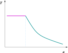
Figure 1: Evolution of the Universe.

To end on an amusing note, consider a phase transition (depicted in fig. 1) between an exponentially expanding (dS) Universe whose bulk dual contains no black hole ($\mu=0$) at constant temperature (46) and our Universe of decreasing temperature (48) which is dual to a Schwarzschild black hole, as we discussed. The transition occurs when the black hole forms. Did the formation of a black hole in the bulk cause the end of inflation?

5 Conclusion

Black holes and their perturbations are a powerful tool in understanding the hydrodynamic behavior of a gauge theory fluid at strong coupling. Bjorken flow can be described in terms of a dual black hole in the bulk. RHIC and the LHC may probe black holes and provide information on string theory as well as non-perturbative QCD effects. The cosmological evolution may also be understood in terms of an AdS₅ Schwarzschild black hole.

References

• [1] de Haro S, Solodukhin S N and Skenderis K 2001 Commun. Math. Phys. 217 595
• [2] Skenderis K 2002 Class. Quant. Grav. 19 5849
• [3] Bjorken J D 1983 Phys. Rev. D 27 140
• [4] Janik R A and Peschanski R 2006 Phys. Rev. D 73 045013
• [5] Janik R A 2007 Phys. Rev. Lett. 98 022302
• [6] Nakamura S and Sin S-J 2006 J. High Energy Phys. JHEP09(2006)020
• [7] Policastro G, Son D T and Starinets A O 2001 Phys. Rev. Lett. 87 081601
• [8] Alsup J and Siopsis G 2008 Phys. Rev. Lett. 101 031602
• [9] Alsup J and Siopsis G 2009 Phys. Rev. D 79 084005
• [10] Apostolopoulos P S, Siopsis G and Tetradis N 2009 Phys. Rev. Lett. 102 151301
• [11] Compère G and Marolf D 2008 Class. Quant. Grav. 25 195014
• [12] Kiritsis E 2005 J. Cosmol. Astropart. Phys. JCAP10(2005)014