Compact binary waveform recovery from the cross-correlated data of two detectors by matched filtering with spinning templates

Abstract

We investigate whether the recovery chances of highly spinning waveforms by matched filtering with randomly chosen spinning waveforms generated with the LAL package are improved by a cross-correlation of the simulated output of the L1 and H1 LIGO detectors. We find that a properly defined correlated overlap improves the mass estimates and enhaces the recovery of spin angles.

1 Method

Recovering a gravitational wave pattern in the noisy detector output is a difficult problem. In this work we present our attempt to recover a gravitational spinning waveform $h_{inj}$ immersed in S5 LIGO-like noise by a modified matched filtering method. We calculate the overlap [1] between the noisy injection $h_{n,i}$ and spinning templates $h_{template}$ as

$$O\left[h_{n,i},h_{template}\right]=\frac{\left\langle h_{n,i}|h_{template}\right\rangle}{\sqrt{\left\langle h_{n,i}|h_{n,i}\right\rangle\left\langle h_{template}|h_{template}\right\rangle}}~{},$$ (1)

with

$$\left\langle h_{1}|h_{2}\right\rangle=4\mathit{Re}\int_{f_{\min}}^{f_{\max}}\frac{\widetilde{h}_{1}\left(f\right)\widetilde{h}_{2}^{\ast}\left(f\right)}{S_{n}\left(f\right)}df~{},$$ (2)

where tilde and star denote Fourier transform and complex conjugate, respectively, and $S_{n}\left(f\right)$ is the power spectral density of the noise. We choose $f_{\min}=50$Hz and $f_{\max}=600$Hz, lying in the best sensitivity band of the LIGO detectors, also the post-Newtonian prediction for the waveform is quite accurate there.

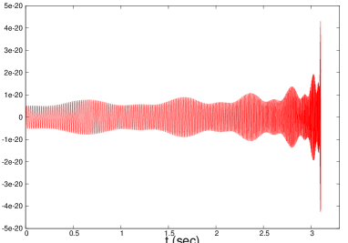
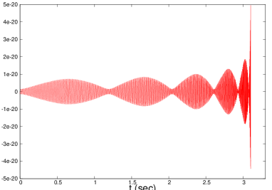
Figure 1: The polarization $h_{+}$ (left) and $h_{\times}$ (right) of the spinning waveforms.

On theoretical grounds, infinite long data series would be required for exact determination of the power spectrum. In order to achieve stability of the power spectral density of order of 1%, we would like to have at least 100 periods of the lowest frequency, therefore a minimal length of the templates of 2 sec was imposed. We compute the above overlap both for the Hanford and Livingston detectors ($O^{H}$ and $O^{L}$, respectively).

We also defined a correlated match, the overlap $O_{corr}^{HL}$, using the correlations of the Hanford and Livingston signals for $h_{n,i}$, $h_{template}$ and noises. (The correlation of $h_{1}$ and $h_{2}$ in Fourier space is defined as $\widetilde{H}\left(f\right)=\widetilde{h}_{1}\left(f\right)\widetilde{h}_{2}^{\ast}\left(f\right)$.)

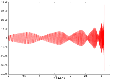
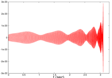
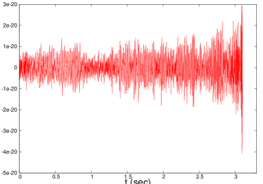
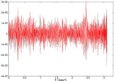
Figure 2: Spinning waveforms at Hanford (top left) and Livingston (top right), mixed in LIGO S5-like noise (bottom).

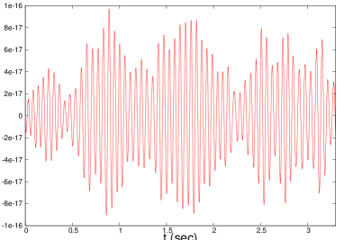
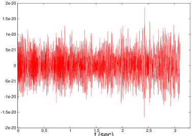
Figure 3: Characteristic unfiltered (left) and filtered (right) LIGO noises.

For the two detectors we also employed the quantity $O^{HL}$, according to Ref. [2]:

$$O^{HL}=\frac{\left\langle h_{n,i}|h_{template}\right\rangle_{H}+\left\langle h_{n,i}|h_{template}\right\rangle_{L}}{\sqrt{\left(\left\langle h_{n,i}|h_{n,i}\right\rangle_{H}+\left\langle h_{n,i}|h_{n,i}\right\rangle_{L}\right)\left(\left\langle h_{template}|h_{template}\right\rangle_{H}+\left\langle h_{template}|h_{template}\right\rangle_{L}\right)}}~{}.$$ (3)

Therefore we could compare four type of matches.

The spinning waveforms, based on Ref. [3], were computed by using SpinTaylor Ref. [4], while the antenna functions based on Ref. [5] with the XLALComputeDetAMResponse() function in DetResponse.c under the LAL package Ref. [4].

Table 1: The parameters of the gravitational wave polarizations ($h_{+},h_{\times}$) of the injected signal. Masses $m_{i}$, magnitude of the dimensionless spins $\chi_{i}$, initial direction of the spin vectors given by $\cos\kappa_{i}$ and $\psi_{i}$ in the frame with the line of sight on the $z$-axis, and the initial orbital angular momentum $\mathbf{L}_{\mathbf{N}}$ in the $x$-$z$ plane, spanning the angle $\Theta$, and the distance $d_{L}$ of the source. The initial phase is $0$; the initial time being also fixed to $0$.

name $m_{1}(M_{\odot})$ $m_{2}(M_{\odot})$ $\chi_{1}$ $\chi_{2}$ $\cos\kappa_{1}$ $\psi_{1}$ $\cos\kappa_{2}$ $\psi_{2}$ $\Theta$ $d_{L}\left(Mpc\right)$ injection $3.553$ $3.358$ $0.983$ $0.902$ $0.984$ $1.109$ $0.978$ $0.957$ $1.430$ $1$

Table 2: The angles $\theta$, $\varphi$ and $\psi$ (polarization angle) give the relation between a fictitious Earth-centered detector and the source frame. For the actual detector positions further rotation have to be taken into account [5]. These angles are also necessary for computing the antenna functions ($F_{+},F_{\times}$). The gravitational signal is $h=h_{+}F_{+}+h_{\times}F_{\times}$.

name $\varphi$ $\theta$ $\psi$ injection $3.657$ $0.278$ $0.000$

Table 1 contains the parameters of the injected waveform. On Fig 1 the two polarizations of this waveform $h_{+}$ and $h_{\times}$ are shown. The parameters characterizing the source and the detector orientation, which are necessary for computing the antenna functions $F_{+}$ and $F_{\times}$ are given in Table 2. The waveforms appearing at the Hanford and Livingston detectors are plotted on Fig 2 (top line), while the bottom line on Fig 2 shows the signals immersed in S5 LIGO-like noise. Some characteristic unfiltered and filtered noises can be seen on Fig 3.

First we calculated the four type of overlaps between the noisy injection and the injected signal itself, finding $O^{H}\left[h_{n,i},h_{injection}\right]=0.8392$, $O^{L}\left[h_{n,i},h_{injection}\right]=0.9064$, $O^{HL}\left[h_{n,i},h_{injection}\right]=0.8662$ and $O_{corr}^{HL}\left[h_{n,i},h_{injection}\right]=0.8646$. Next we defined the following auxiliary quantity for all overlaps

$$\sigma=\left|1-\frac{O\left[h_{n,i},h_{template}\right]}{O\left[h_{n,i},h_{injection}\right]}\right|~{},$$ (4)

vanishing for the injected template. We searched for templates with the various $\sigma$-s less then $0.1$.

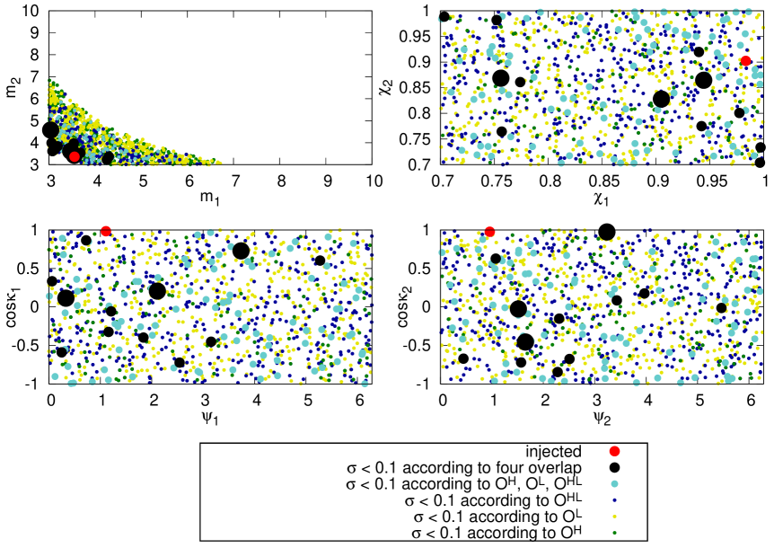
Figure 4: The parameters of  the injected signal (red) and the templates having $\sigma<1$ according to $O^{H}$ (green), $O^{L}$ (yellow), $O^{HL}$ (dark blue) and all of these (light blue) and when the correlated overlap was also taken into account (black). The big dots among the black represent those templates that has the smallest values accordint to the correlated overlap.

The templates were chosen with parameters in the ranges: masses $m_{i}\in$ $3\div 10$ M_⊙; dimensionless spins $\chi_{i}\in 0.7\div 1$; spin angles $\cos\kappa_{i}$ and $\psi_{i}$ random; distance $d_{L}$, angles $\Theta$, $\varphi$, $\theta$ and $\psi$ are fixed identically to the values given in Tables 1 and 2 for the injection, respectively. We also assumed as known the time of signal arrival to the detector. Therefore we varied two mass and six spin parameters altogether.

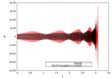
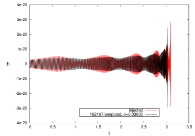
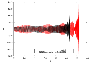
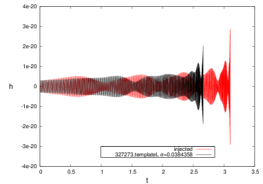
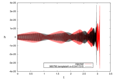
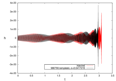
Figure 5: Best three templates (black) as they would appear at Hanford (left) and Livingston (right), compared to the respective injected signals (red).

2 Results

Our analysis is based on matching more than one million templates. The templates with any of the $\sigma^{H}$, $\sigma^{L}$, $\sigma^{HL}$ $<0.1$ were selected and represented on Fig 4 in the parameter planes ($m_{1},m_{2}$), ($\chi_{1},\chi_{2}$) and ($\cos\kappa_{i},\psi_{i}$) for both spins. The green, yellow and navy dots (for grayscale see the legend) represent templates with required values of $\sigma^{H}$, $\sigma^{L}$and $\sigma^{HL}$, respectively; templates with all three values of $\sigma$ below the threshold are plotted with larger turqoise dots. Twelve even larger black dots show templates with all four $\sigma$-s (including $\sigma_{corr}^{HL}$) below the threshold. The three largest of them have the lowest value of $\sigma_{corr}^{HL}$. The parameters of the best three templates are shown in Table 3, and they are plotted on Fig 5 as they would appear at the Hanford and Livingston detectors.

Discussion: The masses are reasonably well recovered, although sligtly overestimated with any of the $\sigma^{H}$, $\sigma^{L}$, $\sigma^{HL}$. The additional monitoring of the correlated match $\sigma_{corr}^{HL}$ imposes however a selection effect which improves the estimation of the masses (top left panel of Fig 4). While the recovery of the spin magnitudes is still problematic (top right panel of Fig 4), the estimation of the spin angles seems slightly improved by the use of of the correlated match $\sigma_{corr}^{HL}$. (Black dots exhibit a belt-like structure on both bottom panels of Fig 4.) How relevant is this feature statistically is currently under investigation.

Table 3: The parameters of the templates represented by the four big black points on Fig 4.

name $m_{1}(M_{\odot})$ $m_{2}(M_{\odot})$ $\chi_{1}$ $\chi_{2}$ $\cos\kappa_{1}$ $\psi_{1}$ $\cos\kappa_{2}$ $\psi_{2}$ 162197.template $3.471$ $3.612$ $0.905$ $0.828$ $0.114$ $0.330$ $-0.026$ $1.515$ 327273.template $3.038$ $4.572$ $0.944$ $0.864$ $0.729$ $3.736$ $-0.455$ $1.652$ 980790.template $3.549$ $3.426$ $0.756$ $0.868$ $0.206$ $2.110$ $0.974$ $3.237$ 281270.template $3.057$ $3.989$ $0.703$ $0.989$ $-0.057$ $1.209$ $-0.721$ $1.569$   

Acknowledgements: This work was supported by the Polányi Program of the Hungarian National Office for Research and Technology (NKTH) and the Hungarian Scientific Research Fund (OTKA) grant no. 69036.

References

• [1] B. Vaishnav, I. Hinder, F. Herrmann, D. Shoemaker, Phys. Rev. D 76 084020 (2007)
• [2] V. Raymond, M. V. van der Sluys, I. Mandel, V. Kalogera, C. Roever, N. Christensen, arXiv:0912.3746 (2009)
• [3] A. Buonanno, Y. Chen, M. Vallisneri, Phys. Rev. D 67 104025 (2003); Erratum-ibid. D 74 029904 (2006)
• [4] https://www.lsc-group.phys.uwm.edu/daswg/projects/lal.html
• [5] W. G. Anderson, P. R. Brady, J. D. E. Creighton, É. É. Flanagan, Phys. Rev. D 63 042003 (2001)