Decoherence as attenuation of mesoscopic echoes in a spin-chain channel

Abstract

An initial local excitation in a confined quantum system evolves exploring the whole system, returning to the initial position as a mesoscopic echo at the Heisenberg time. We consider a two weakly coupled spin chains, a spin ladder, where one is a quantum channel while the other represents an environment. We quantify decoherence in the quantum channel through the attenuation of the mesoscopic echoes. We evaluate decoherence rates for different ratios between sources of amplitude fluctuation and dephasing in the inter-chain interaction Hamiltonian. The many-body dynamics is seen as a one-body evolution with a decoherence rate given by the Fermi golden rule.

I Introduction

Control of quantum dynamics is essential to achieve quantum information processing. Examples of this are implementations of quantum algorithms z–Grover ; z-Shor and quantum communications z–teleportI ; z–teleportII . The system involved in each of these processes interacts with an environment which degrades the quantum correlations z–Zurek . This loss of information, called decoherence, represents the main obstacle to achieve an efficient quantum processing. Thus, in order to avoid decoherence, it is mandatory to understand its processes. Many approaches exist to study decoherence in systems composed by few qubits Koppens06 ; Wu06 ; Grajcar06 ; Riebe06 . However, real computer implementations that involve large number of qubits require the development of new approaches to characterize decoherence Krojanski04 ; Krojanski06 ; AlvarezPRL10 .

Recently, many efforts were done to characterize the quantum noise Chuang00 ; z–Guo ; z–BoseDeco that produces decoherence in quantum channels. These channels connect two quantum systems enabling the information transfer between them. Spin chains can be used to achieve this goal for short distance communications z–Bose avoiding interfaces between the static system and the information carriers. Whereas all these studies were oriented to pure-state communication processes, experimental realizations of pure-state dynamics are a major challenge z–QCRoadmap04 . Alternatively, implementations of quantum computation with NMR can not deal with pure states but have to resort to statistical mixtures of spin ensembles instead Cory97 ; Chuang97 ; Laflame98 . State transfer in spin ensembles was done in a ring of spins with many-body interactions in the solid state z–EcosMesoscI ; z–EcosMesoscII . An initial local polarization propagates around the ring. The return of the initial excitation is evidenced through the constructive interference that reappears at the Heisenberg time $t_{\mathrm{H}}\sim\hbar/\Delta$, with $\Delta$ the typical mean energy level spacing, as a form of polarization revival called the mesoscopic echo z–ME-Altshuler . There, the polarization amplitude and phase of a given nuclear spin within the ring was monitored as a function of time. However, the many body nature of spin-spin interactions strongly compromises an optimum transfer. Thus, a much more efficient transfer was observed through the experimental implementation of an effective $XY$ Hamiltonian (i.e. flip-flop processes) in a spin chain z–Madi by exploiting the $J$-coupling in the liquid phase, where dipolar interaction becomes negligible. The main reason for this result is that the many-body dynamics of an $XY$ Hamiltonian is mappable to a one-body evolution Lieb61 . Thus, in this case, the Heisenberg time is proportional to the system size $M$ instead of the $2^{M}$ value that shows in a complex many-body Hamiltonian. In Ref. z–Madi , the evolution of the initial excitation was monitored in all the spins of the quantum channel. Comparisons with theoretical calculations showed the effect of decoherence manifested in the attenuation of the interference intensities which is more evident in the decay of the mesoscopic echoes. This experimental breakthrough enabled various theoretical proposals for perfect state transfer Christandl04 ; Stolze05 . More recently, implementations of spin-chains were done in solid-state NMR CapellaroPRA07 by implementing a Double Quantum Hamiltonian (i.e. flip-flip+flop-flop processes) which, in turn, is mappable to an XY interaction Doronin . However, the progress toward the proposal to observe the mesoscopic echoes of these systems CapellaroPRL07 was experimentally limited by length inhomogeneity Rufeil-Fiori-MQC .

In this work we propose to use the attenuation of the mesoscopic echoes in a spin chain as a sensor of the decoherence produced by an uncontrolled spin bath, in this case a second spin chain. The spin-spin interaction within each chain is given by an $XY$ Hamiltonian where the ensemble dynamics can be solved analytically z–FeldmanErnst ; z-SPC ; z–NuestroCPL05 . Once the chains are laterally coupled to form a spin ladder, the quantum dynamics becomes truly many-body and the analytical solution is no longer possible. Moreover, numerical solutions are difficult to obtain as a consequence of the exponential increase of the Hilbert space dimension Quantum-Paralelism . We show that, within certain range of the ratio between the inter-chain and intra-chain interactions, the evolution of a local excitation in the many-body system (spin ladder) can be obtained as a one-body dynamics (isolated chain evolution) plus a decoherence process given by a Fermi golden rule (FGR). We characterize the decoherence rate for different kinds of inter-chain interactions by controlling the contribution of the different sources: pure dephasing (Ising interaction) and amplitude fluctuations ($XY$ interaction). Thus, we show that this auto-correlation function becomes an effective and practical tool for studying decoherence. Moreover, the exploration nature of the mesoscopic echo provides the sender (Alice) with the information of the decoherence effects in the quantum channel by contrasting with the expected result of the isolated dynamics. This could enable the implementation of a convenient error correction code without needing of a receiver.

In the next section, we introduce the system and present the numerical calculations of the local polarization evolution for different inter-chain interactions. From these results we obtain the decoherence rates from the attenuation of the mesoscopic echoes. In the third section, for a solvable small system, we characterize analytically the decoherence rates. Instead of using the quantum master equation which is the most standard framework adopted to describe the system-environment interaction z–QmasterE1 ; z–QmasterE2 , we use the Keldysh non-equilibrium formalism which leads to an integral solution of the Schrödinger equation z-SPC ; z–NuestroCPL05 ; z–NuestroSSC07 ; z–NuestroPRA07 . Finally, we discuss the conclusions.

II Spin dynamics in a non-isolated spin-chain channel

II.1 System

Let us consider the polarization dynamics in a spin system composed by two parallel spin chains transversely coupled. The topology of the interaction network forms a ladder. Chain I represents the quantum channel composed by $M$ spins, and chain II is another $M$ spin system that perturbs the quantum transfer in chain I, see Fig. 1(a). The spin Hamiltonian is given by

$$\widehat{\mathcal{H}}_{\mathrm{total}}=\widehat{\mathcal{H}}_{\mathrm{I}}+\widehat{\mathcal{H}}_{\mathrm{II}}+\widehat{\mathcal{H}}_{\mathrm{T}},$$ (1)

where

$$\widehat{\mathcal{H}}_{\mathrm{\alpha}} =\sum_{n=1}^{M-1}J_{n+1,n}^{(\mathrm{\alpha})}\left(\widehat{S}_{n+1}^{{}_{(\mathrm{\alpha})}x\ }\widehat{S}_{n}^{{}_{(\mathrm{\alpha})}x}+\widehat{S}_{n+1}^{{}_{(\mathrm{\alpha})}y\ }\widehat{S}_{n}^{{}_{(\mathrm{\alpha})}y}\right)$$ (2)

$$=\sum_{n=1}^{M-1}\frac{J_{n+1,n}^{(\mathrm{\alpha})}}{2}\left(\widehat{S}_{n+1}^{{}_{(\mathrm{\alpha})}+\ }\widehat{S}_{n}^{{}_{(\mathrm{\alpha})}-}+\widehat{S}_{n+1}^{{}_{(\mathrm{\alpha})}+\ }\widehat{S}_{n}^{{}_{(\mathrm{\alpha})}-}\right)$$ (3)

represents the $\mathrm{\alpha}$-th spin chain Hamiltonian that takes into account the $XY$ interaction between neighbor 1/2-spins within the chain. The spin chains interact through the following transversal Hamiltonian

$$\widehat{\mathcal{H}}_{\mathrm{T}} =\sum_{n=1}^{M}aJ_{n}\widehat{S}_{n}^{{}_{(\mathrm{I})}z}\widehat{S}_{n}^{{}_{(\mathrm{II})}z}+bJ_{n}\left(\widehat{S}_{n}^{{}_{(\mathrm{I})}x}\widehat{S}_{n}^{{}_{(\mathrm{II})}x}+\widehat{S}_{n}^{{}_{(\mathrm{I})}y}\widehat{S}_{n}^{{}_{(\mathrm{II})}y}\right)$$ (4)

$$=\sum_{n=1}^{M}aJ_{n}\widehat{S}_{n}^{{}_{(\mathrm{I})}z}\widehat{S}_{n}^{{}_{(\mathrm{II})}z}+\frac{bJ_{n}}{2}\left(\widehat{S}_{n}^{{}_{(\mathrm{I})}+}\widehat{S}_{n}^{{}_{(\mathrm{II})}-}+\widehat{S}_{n}^{{}_{(\mathrm{I})}+}\widehat{S}_{n}^{{}_{(\mathrm{II})}-}\right),$$ (5)

where by controlling the ratio $a/b$ one determines the nature of the interaction. The polarization evolution is considered for different transversal interactions: $XY$ interaction ($a/b=0$); isotropic (Heisenberg) interaction ($a/b=1$); and truncated dipolar interaction ($a/b=-2$), which are typical in NMR experiments z–QmasterE1 ; z–QmasterE2 . Besides these three typical NMR interactions we will also consider the evolution under two additional transversal Hamiltonian with the following parameters $H_{1}$ ($a/b=2$) and $H_{2}$ ($a/b=3.6$). We will focus on regular systems where all longitudinal couplings within chains are taken equals $J_{n+1,n}^{(\mathrm{\alpha})}=J_{\mathrm{x}}$ $(n\neq M)$. The same is applied to the transversal couplings $J_{n}=J_{\mathrm{y}}$. We choose these parameter conditions because the interference effects are more pronounced and the mesoscopic echo degradation can be easily evaluated.

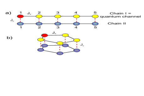
Figure 1: (Color online): (a) Schematic representation of the spin ladder system given by the Hamiltonian of Eq. (1). Each spin chain has $M=5$ spins. (b) A system like in (a) but with periodic boundary conditions between spins $1$ and $M$. Light colors represent the quantum channel. Marked spin (red online) represents the site where the initial condition is placed.

II.2 Decoherence characterization based on the attenuation of mesoscopic echoes

In order to study the mesoscopic echoes of a spin ensemble, we calculate the evolution of a local polarization within chain I (quantum channel) through the spin auto-correlation function z-SPC ; z–NuestroCPL05 ,

$$P_{1,1}(t)=\frac{\left\langle\Psi_{\mathrm{eq}}\right|\widehat{S}_{1}^{{}_{(\mathrm{I})}z}(t)\widehat{S}_{1}^{{}_{(\mathrm{I})}z}(0)\left|\Psi_{\mathrm{eq}}\right\rangle}{\left\langle\Psi_{\mathrm{eq}}\right|\widehat{S}_{1}^{{}_{(\mathrm{I})}z}(0)\widehat{S}_{1}^{{}_{(\mathrm{I})}z}(0)\left|\Psi_{\mathrm{eq}}\right\rangle}.$$ (6)

This gives the local polarization in the $z$ direction on site $1$ at time $t$ providing that the system was in its equilibrium state plus a local excitation on site $1$ at time $t=0$. Here, $\widehat{S}_{1}^{{}_{(\mathrm{\alpha})}z}\left(t\right)=e^{\mathrm{i}\widehat{\mathcal{H}}_{\mathrm{total}}t/\hbar}\widehat{S}_{1}^{{}_{(\mathrm{\alpha})}z}e^{-\mathrm{i}\widehat{\mathcal{H}}_{\mathrm{total}}t/\hbar}$ is the spin operator in the Heisenberg representation and $\left|\Psi_{\mathrm{eq}}\right\rangle$ is the many-body state corresponding to thermal equilibrium, that is a mixture with appropriate statistical weights, of all possible states with different number $N$ of spins up. In the regime of NMR spin dynamics $k_{\mathrm{B}}T$ is much higher than any energy scale of the system. Then, all the statistical weights can be taken equal z–QmasterE1 ; z–QmasterE2 . As numerical method we alternate between the standard diagonalization by spin projection subspaces z–EcosMesoscI or the Quantum Parallelism algorithm Quantum-Paralelism , which involves the evolution of a few superposition states representing the whole ensemble. Although the last is much more efficient for larger samples, for the considered system sizes, both involve similar computing time. As the results coincide, no further comment is devoted to this point.

By assuming $J_{\mathrm{y}}$ equal to zero, the local polarization dynamics at spin $1$ in chain I is equivalent to the local evolution in an isolated spin chain, $P_{1,1}^{\text{{isolated}}}(t)$. This function is defined with Eq. (6) replacing $\widehat{\mathcal{H}}_{\mathrm{total}}$ by $\widehat{\mathcal{H}}_{\mathrm{I}}$ and $\widehat{S}_{1}^{{}_{(\mathrm{I})}z}\left(t\right)=e^{\mathrm{i}\widehat{\mathcal{H}}_{\text{{I}}}t/\hbar}\widehat{S}_{1}^{{}_{(\mathrm{I})}z}e^{-\mathrm{i}\widehat{\mathcal{H}}_{\text{{I}}}t/\hbar}$. Since the $XY$ spin-spin interaction within the chain only couples nearest neighbors, the system dynamics in the high temperature regime can be obtained analytically as a one-body dynamics z-SPC ; z–NuestroCPL05 . Upper line (black) in Figure 2(a) shows the solution of $P_{1,1}^{\text{{isolated}}}(t)$ for a spin chain with $M=5$. We can observe the presence of the $k$-th mesoscopic echo at a time $t_{k}^{\text{{ME}}}$ proportional to the chain size $M$ z–EcosMesoscI . As $J_{\mathrm{y}}$ increases, the degrees of freedom of chain II start modifying the observed dynamics of $P_{1,1}^{\text{{isolated}}}(t)$ and, in general, no analytical solution is known. To obtain the polarization dynamics $P_{1,1}(t)$ of this many-body problem, we solve numerically the time dependent Schrödinger equation by using the Trotter-Suzuki decomposition z–DeRaedt . Color curves of Fig. 2(a) show the local polarization $P_{1,1}(t)$ for different values of $J_{\mathrm{y}}$ corresponding to an isotropic transversal Hamiltonian. They evidence the degradation of mesoscopic echoes proportionally to $J_{\mathrm{y}}$. Fig. 2(b) shows $P_{1,1}(t)$ for different forms of the transversal interaction Hamiltonian for a fixed value of $J_{\mathrm{y}}$. Due to the $XY$ term in the transversal Hamiltonian, the polarization is transferred back and forth between chain I and II. This process, plus the dephasing induced by the Ising contribution, produce the progressive spreading of the polarization among all the spins thus degrading the strong recurrences. This is manifested in the mean value of the local polarization at longer times, $t\gg\hbar/J_{\mathrm{x}},$ that approximately tends to $1/\left(2M\right)$. Thus, one observes a decrease of the mesoscopic echoes with evolution time as well as a gradual increase of the background polarization at times between echoes. We do not consider an Ising transversal interaction ($b/a=0$) since it does not involve transfer of polarization between chains leading to a different value of the mean local magnetization at long times. In the latter case, the mean local polarization at long times tends to a value that is close to $1/M$ instead of the $1/\left(2M\right)$ value. This difference in the final state avoid a direct comparison with the polarization dynamics from Hamiltonians that contain an $XY$ term requiring extra manipulations.

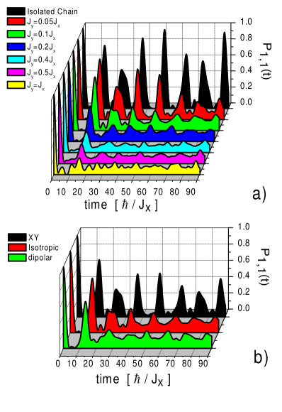
Figure 2: (Color online): Polarization at site $1$, $P_{1,1}(t)$, of the spin ladder of Fig 1(a). (a) Upper (black) curve represents the dynamics of an isolated chain given by $P_{1,1}^{\text{{isolated}}}(t)$. Color curves correspond to different values of the coupling $J_{\mathrm{y}}$ for a transversal isotropic interaction between chains. (b) Comparison of the dynamics behavior between different transversal interaction natures ($XY$, Isotropic, dipolar) by keeping fixed the coupling ratio $J_{\mathrm{y}}/J_{\mathrm{x}}=0.1$.

In order to characterize decoherence of the quantum channel, we measure the attenuation of the mesoscopic echoes as compared with the local polarization in the isolated spin-chain channel, $P_{1,1}^{\text{{isolated}}}(t)$. Figure 2 shows that the ratio $P_{1,1}(t_{k}^{\text{{ME}}})/P_{1,1}^{\text{{isolated}}}(t_{k}^{\text{{ME}}})$ decreases as a function of $t_{k}^{\text{{ME}}}$. Within the regime $\left|J_{\mathrm{y}}/J_{\mathrm{x}}\right|\ll 1$ we observe that this ratio has an exponential dependence of the form $\exp[-t_{k}^{\text{{ME}}}/\tau_{\phi}]$. This exponential decay of the initial polarization cannot hold for all times until $P_{1,1}(t)=0$ since the system size is finite and the total polarization is conserved within the system. Thus, for a later time the correlations within chain II are manifested at site $1$, and the ratio $P_{1,1}(t_{k}^{\text{{ME}}})/P_{1,1}^{\text{{isolated}}}(t_{k}^{\text{{ME}}})$ evidences a complex behavior instead of an exponential one. The numerical results show that the crossover between the two temporal behavior appears at times proportional to $t_{\mathrm{R}}\propto\tau_{\phi}\ln[J_{x}\tau_{\phi}/\hbar]$ z–elenaCPL05 . To characterize the exponential decay of the mesoscopic echoes we calculate the ratio $P_{1,1}(t_{k}^{\text{{ME}}})/P_{1,1}^{\text{{isolated}}}(t_{k}^{\text{{ME}}})$ for several values of $t_{k}^{\text{{ME}}}$ previous to this crossover time. The accuracy of this characterization improves proportionally to the order $k$ of the mesoscopic echo. Thus, to avoid dealing with too long times or large number of spins, we increase the order of observable echoes without changing the physical behavior of the system by putting periodic boundary condition in $\widehat{\mathcal{H}}_{\mathrm{I,II}}$. This “closes” the spin chain into a ring as shown in figure 1(b). This choice approximately duplicate the number of mesoscopic echoes for a fixed evolution time with respect to the observed in the chain.

Since chain II does not have infinite degrees of freedom it does not represent a reservoir. Thus, the presence of recurrences in the quotient $P_{1,1}(t_{k}^{\text{{ME}}})$/$P_{1,1}^{\mathrm{isolated}}(t_{k}^{\text{{ME}}})$ is expected instead of an exponential law. In figure 3, the function $-\log(P_{1,1}(t)/P_{1,1}^{\mathrm{isolated}}(t))$ is plotted for different values of $J_{\mathrm{y}}$ as a function of time. Due to the dynamics within the channel each curve oscillates around zero. The maximum values are associated to the temporal region where $P_{1,1}^{\mathrm{isolated}}(t)>P_{1,1}(t)$, that is, the region where the mesoscopic echoes are manifested. The minimum values, on the other hand, correspond to the temporal regions between mesoscopic echoes, where $P_{1,1}^{\mathrm{isolated}}(t)<P_{1,1}(t)$. It can be seen that an exponential law is identified in the envelop of the peaks that appears for each curve (see dashed line). In figure 4 are plotted the values of the maxima of figure 3 for $J_{\mathrm{y}}=0.09J_{\mathrm{x}}$ and $J_{\mathrm{y}}=0.10J_{\mathrm{x}}$ as a function of time. The peaks start to get apart from its envelop at different times proportional to $t_{\mathrm{R}}$ depending on the intensities of the transverse interaction. This behavior reflects the recurrences due to the finite nature of chain II, which becomes relevant for earlier times as the intensities $J_{\mathrm{y}}$ increases. In order to quantify the exponential behavior corresponding to each value of the transverse interaction $J_{\mathrm{y}}$, we fit the maximum values shown in Fig. 4 to a linear function. Thus, we extract the decoherence time $\tau_{\phi}$ from the slope of the curve for different values of the transversal interaction $J_{\mathrm{y}}$. The number of points (number of echoes) used in this procedure varies depending on the value of $J_{\mathrm{y}}$ as can be seen in Fig. 4. Besides, the point $(0,0)$ is not included in the fit since for very short times $t\ll\hbar/J_{\mathrm{x}}$ the behavior of quantum dynamics is not exponential but it starts quadratic with $t$.

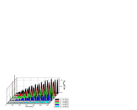
Figure 3: (Color online): Natural logarithm of the ratio $P_{11}(t)/P_{1,1}^{\text{{isolated}}}(t)$ for different values of the transversal coupling $J_{\mathrm{y}}$ as a function of time. The interaction between chains has an isotropic nature. The dashed line is a guide to the eye.

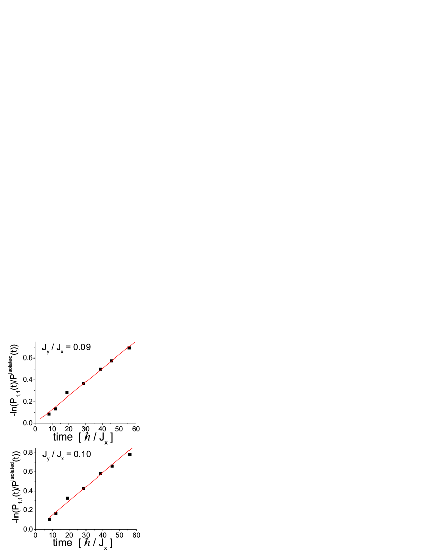
Figure 4: (Color online): Maximum values of Fig. 3 for two different ratios $J_{\mathrm{y}}/J_{\mathrm{x}}$ as a function of time. The slope of the linear fit (solid line) gives the value of $\tau_{\phi}$ associated to the perturbation $J_{\mathrm{y}}$.

The existence of an exponential law in the decay of the mesoscopic echoes where $\tau_{\phi}\propto\left|\hbar J_{\mathrm{x}}/J_{\mathrm{y}}^{\ 2}\right|$ plus the fact that its time regime is bounded by a time proportional to $t_{\mathrm{R}}\propto\tau_{\phi}\ln[J_{x}\tau_{\phi}/\hbar]$ suggests that the decay of mesoscopic echoes in chain I could be described by the Self Consistent Fermi Golden Rule (SC-FGR) analyzed in Ref. z–elenaCPL05 .

Figure 5 shows the obtained values of $\tau_{\phi}$ as a function of $\frac{\left|J_{\mathrm{y}}\right|^{2}}{\hbar J_{\mathrm{x}}}$ evidencing a linear dependence. The curves correspond to transversal interaction of different nature by varying the ratio $a/b$ in Eq. (4): $XY$ ($a/b=0$), isotropic or Heisenberg ($a/b=1$), truncated dipolar ($a/b=-2$), $H_{1}$ ($a/b=2$) and $H_{2}$ ($a/b=3.6$). The slopes of the linear curves are shown in table 1.

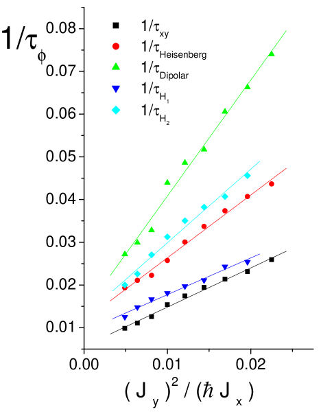
Figure 5: (Color online): Decoherence rates $\frac{1}{\tau_{\phi}}$ for different transversal Hamiltonians as a function of $\left|J_{\mathrm{y}}\right|^{2}/\hbar J_{\mathrm{x}}$. The lineal dependence indicates the good agreement with the FGR behavior. Different slopes indicate that the decoherence rate is composed by two contributions: One is due to the injection of polarization produced by the $XY$ term of $\widehat{\mathcal{H}}_{\mathrm{T}}$ and the other is associated to the dephasing process given by the Ising term.

$\widehat{\mathcal{H}}_{\mathrm{T}}$	$\frac{1}{\tau_{\phi}}$
$XY$ ($a/b=0$)	$\left(0.96\pm 0.04\right)\frac{\left|J_{\mathrm{y}}\right|^{2}}{\hbar J_{\mathrm{x}}}$
Isotropic ($a/b=1$)	$\left(1.47\pm 0.05\right)\frac{\left|J_{\mathrm{y}}\right|^{2}}{\hbar J_{\mathrm{x}}}$
dipolar ($a/b=-2$)	$\left(2.7\pm 0.1\right)\frac{\left|J_{\mathrm{y}}\right|^{2}}{\hbar J_{\mathrm{x}}}$
$H_{1}$ ($a/b=2$)	$\left(0.81\pm 0.04\right)\frac{\left|J_{\mathrm{y}}\right|^{2}}{\hbar J_{\mathrm{x}}}$
$H_{2}$ ($a/b=3.6$)	$\left(1.8\pm 0.1\right)\frac{\left|J_{\mathrm{y}}\right|^{2}}{\hbar J_{\mathrm{x}}}$

Table 1: Proportional constants between $1/t_{\phi}$ and $|J_{y}|^{2}/(\hbar J_{x})$ for different interactions between chains.

The linear behavior observed in figure 5 confirms that, even when we are dealing with closed systems in which the energetic spectrum of the environment (chain II) is not continuous, the characteristic time $\tau_{\phi}$ agrees with the one dictated by the FGR. The conditions needed to derive the FGR in molecular spin systems was already addressed in ref. z–elenaCPL05 . There, the behavior of the numerical simulations on clusters with less than $20$ spins for times shorter than $t_{\mathrm{H}}$ was observed to coincide perfectly with the theoretical results.

In the present case, $5+5$ spins, the unperturbed Hamiltonian is represented by $\widehat{\mathcal{H}}_{\mathrm{I}}+\widehat{\mathcal{H}}_{\mathrm{II}}$, while the perturbation is $\widehat{\mathcal{H}}_{\mathrm{T}}$. The initial state is not an eigenstate of $\widehat{\mathcal{H}}_{\mathrm{I}}+\widehat{\mathcal{H}}_{\mathrm{II}}$, but instead it is a superposition of the $2^{5}$ eigenstates of chain I. Since the initial state is spatially localized, all the eigenstates of chain I contribute with equal weight to this superposition. Therefore, the decay of a local polarization involves a sort of average over all possible initial and final states. This justifies the use of the expression for the characteristic time given by the Fermi Golden Rule Pascazio99

$$\frac{1}{\tau_{\phi}}\simeq\frac{2\pi}{\hbar}\left\|\widehat{\mathcal{H}}_{\mathrm{T}}\right\|^{2}N_{0},$$ (7)

where $\left\|\widehat{\mathcal{H}}_{\mathrm{T}}\right\|$ is a characteristic value of the coupling interactions between chains that has to be determined and $N_{0\text{ }}$represents the density of directly connected states, i.e. states of the states of chain II connected with the initial state through the perturbation $\widehat{\mathcal{H}}_{\mathrm{T}}$. This interaction consists of two processes: the flip-flop (or $XY)$ interaction and the Ising interaction weighted by the factors $a$ and $b$ respectively. Thus, the evolution of the initial localized state generated in chain I decays due to the coupling with the “environment” represented by chain II. Equation (7) involves the assumption that $N_{0\text{ }}$is similar for the $XY$ and Ising interaction, i.e., $N_{0}^{\mathrm{XY}}=N_{0}^{\mathrm{ZZ}}=N_{0}$. This density of states can be approximated as the inverse of the second moment of $\widehat{\mathcal{H}}_{\text{{II}}}$, and then $N_{0}\propto 1/J_{\mathrm{x}}$. The cross terms proportional to $ab$ are canceled out in $\left\|\widehat{\mathcal{H}}_{\mathrm{T}}\right\|^{2}$ z–QmasterE1 , thus, under these approximations each interaction terms between chains becomes independent of each other obtaining

$$\frac{1}{\tau_{\phi}}=\frac{1}{\tau_{\phi}^{\mathrm{ZZ}}}+\frac{1}{\tau_{\phi}^{\mathrm{XY}}},$$ (8)

with

$$\frac{1}{\tau_{\phi}^{\mathrm{ZZ}}}=Aa^{2}\frac{\left|J_{\mathrm{y}}\right|^{2}}{\hbar J_{\mathrm{x}}}\text{ and{ }}\frac{1}{\tau_{\phi}^{\mathrm{XY}}}=Bb^{2}\frac{\left|J_{\mathrm{y}}\right|^{2}}{\hbar J_{\mathrm{x}}},$$ (9)

where $A$ and $B$ represent constants associated with each interaction. We determine these constants by using the numerical results of table 1. Equation (8) can be rewritten as

$$y_{\mathrm{XY}}=-\frac{A}{B}x_{\mathrm{ZZ}}+\frac{1}{B}$$ (10)

where $x_{\mathrm{ZZ}}=a^{2}\tau_{\phi}\left|J_{\mathrm{y}}\right|^{2}/\left(\hbar J_{\mathrm{x}}\right)$ and $y_{\mathrm{XY}}=b^{2}\tau_{\phi}\left|J_{\mathrm{y}}\right|^{2}/\left(\hbar J_{\mathrm{x}}\right)$. Figure (6) shows the curve $y_{\mathrm{XY}}$ vs. $x_{\mathrm{ZZ}}$ (squares) for the three standard NMR Hamiltonians, $XY$ ($b=1$, $a=0$), Isotropic ($b=1$, $a=1$), dipolar ($b=1,a=-2$) and for other two arbitrary Hamiltonians $\widehat{\mathcal{H}}_{1}$ and $\widehat{\mathcal{H}}_{2}$ with parameters ($b=0.5,$ $a=1$) and ($b=0.5,$ $a=1.8$) respectively. By doing a linear fitting (solid line), we obtain

$$A=(0.49\pm 0.08)\text{ and{ }}B=(1.00\pm 0.06)$$ (11)

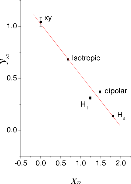
Figure 6: (Color online): $y_{\mathrm{XY}}$ vs. $x_{\mathrm{ZZ}}$ for different natures of the transversal interaction, where $x_{\mathrm{ZZ}}=a^{2}\tau_{\phi}\left|J_{\mathrm{y}}\right|^{2}/\left(\hbar J_{\mathrm{x}}\right)$ and $y_{\mathrm{XY}}=b^{2}\tau_{\phi}\left|J_{\mathrm{y}}\right|^{2}/\hbar J_{\mathrm{x}}$. The solid line is given by a linear fitting to the points.

It is important to note that the role of the interaction nature on the decoherence time is manifested through the constants $A$ and $B$. The origin of this factors will be clarified in the next section by using the Keldysh form of the quantum field many-body theory. There, a microscopic model is applied to a similar spin system. We will obtain analytical expressions that agree well with the numerical values obtained here.

III Two-spin channel coupled to a spin bath: Analytical solution

III.1 System

In this section, we consider the simplest quantum spin channel: a two spin system that could act as a SWAP gate. Each of these spins is coupled with an independent spin environment as is sketched in Fig. 7. Since the system describes a Rabi oscillation that could be damped by the interaction of the spin bath, it contains all the essential ingredients of the spin channel case, with the further advantage that it could be solved analytically and to asses in detail how the environment disturbs it. Therefore, it allows the exact characterization of the decoherence rate in order to compare with the numerical results of the previous section.

The Hamiltonian of the two spin system is given by $\widehat{\mathcal{H}}_{\mathrm{I}}$ of Eq. (2) with $M=2$. The system-environment Hamiltonian is equivalent to Eq. (4) with $M=2$. Finally, the environment is represented by two independent and semi-infinite linear chains whose Hamiltonians are given by $\widehat{\mathcal{H}}_{\mathrm{II}}$ of Eq. (2) with $M\rightarrow\infty.$ By neglecting the interaction between the semi-infinite portions we ensure that no correlation could appear. We call them $\widehat{\mathcal{H}}_{\mathrm{EL}}$ and $\widehat{\mathcal{H}}_{\mathrm{ER}},$ see figure 7. As the theoretical framework we adopt the Keldysh formalism z–Danielewicz in a form that was developed for electronic excitations z–GLBEI ; z–GLBEII and then extensively developed to solve the spin dynamics in presence of system-environment interactions z-SPC ; z–NuestroCPL05 ; z–NuestroSSC07 ; z–NuestroPRA07 . More recently, this formalism also proved to be useful to address thermal transport Arrachea-Lozano-Aligia .

In this work, we briefly discuss the main points of the formalism required to arrive to the solution. We start by establishing the relation between spin and fermion operators at a given site $n$ by applying the Jordan-Wigner transformation (JWT) Lieb61

$$\widehat{S}_{n}^{+}=\widehat{c}_{n}^{+}\exp\{\mathrm{i}\pi\sum_{m=1}^{n-1}\widehat{c}_{m}^{+}\widehat{c}_{m}\}.$$ (12)

Here, $\widehat{c}_{n}^{+}$ and $\widehat{c}_{n}$ stand for the creation and destruction fermionic operators, and $\widehat{S}_{n}^{\pm}$ are the rising and lowering spin operator, $\widehat{S}_{n}^{\pm}=\widehat{S}_{n}^{x}\pm\mathrm{i}\widehat{S}_{n}^{y}$. Within the fermionic description, the spin-up and spin-down states correspond to an occupied and not-occupied fermionic state respectively.

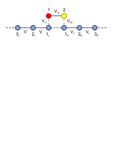
Figure 7: (Color online): Schematic representation of the two spin channel coupled to independent spin environments.

After applying the JWT to the total two spin Hamiltonian

$$\widehat{\mathcal{H}}^{2\text{-}\mathrm{spin}}=\widehat{\mathcal{H}}_{\mathrm{I}}+\widehat{\mathcal{H}}_{\mathrm{T}}+\widehat{\mathcal{H}}_{\mathrm{EL}}+\widehat{\mathcal{H}}_{\mathrm{ER}},$$ (13)

it is possible to rewrite the different contributions of $\widehat{\mathcal{H}}^{2\text{-{spin}}}$. $\widehat{\mathcal{H}}_{\mathrm{I}}$ is given by

$$\widehat{\mathcal{H}}_{\mathrm{I}}=V_{12}\left(\hat{c}_{1}^{+}\hat{c}_{2}+\hat{c}_{2}^{+}\hat{c}_{1}\right),$$ (14)

where the hopping amplitude between states $1$ and $2$ is

$$V_{12}\equiv J/2$$

and the transition between them occurs at the natural Rabi frequency

$$\omega_{0}=2V_{12}/\hbar.$$ (15)

The environment is represented by

$$\widehat{\mathcal{H}}_{\mathrm{EL}}+\widehat{\mathcal{H}}_{\mathrm{ER}}=\sum_{i=1}^{\infty}V_{\mathrm{L}}\left(\hat{c}_{\mathrm{L,}i}^{+}\hat{c}_{\mathrm{L},i+1}+\hat{c}_{\mathrm{L},i+1}^{+}\hat{c}_{\mathrm{L},i}\right)\\ +\sum_{i=1}^{\infty}V_{\mathrm{R}}\left(\hat{c}_{\mathrm{R},i}^{+}\hat{c}_{\mathrm{R},i+1}+\hat{c}_{\mathrm{R},i+1}^{+}\hat{c}_{\mathrm{R},i}\right),$$ (16)

where $\hat{c}_{\mathrm{L},i}^{+}(\hat{c}_{\mathrm{L},i})$ is the creation (destruction) fermionic operator for the environment that interacts with the system state $1$ and similarly for $\hat{c}_{\mathrm{R},i}^{+}(\hat{c}_{\mathrm{R},i})$ which belongs to the environment that interacts with the system state $2$. $V_{\mathrm{L}}$ and $V_{\mathrm{R}}$ stand for the hopping term between neighboring sites within each of the environments. They correspond to the XY (flip-flop) interaction along the $x$ direction.

$$V_{\mathrm{L}}=V_{\mathrm{R}}\equiv J_{\mathrm{x}}/2\leavevmode\nobreak\ .$$ (17)

Finally, the transversal or system-environment interaction takes the form

$$\widehat{\mathcal{H}}_{\mathrm{T}}=V_{1\mathrm{L}}^{\mathrm{XY}}\leavevmode\nobreak\ (\hat{c}_{\mathrm{L},1}^{+}\hat{c}_{1}+\hat{c}_{1}^{+}\hat{c}_{\mathrm{L},1})\\ +V_{1\mathrm{L}}^{\mathrm{ZZ}}\leavevmode\nobreak\ \left[\hat{c}_{\mathrm{L},1}^{+}\hat{c}_{\mathrm{L},1}\hat{c}_{1}^{+}\hat{c}_{1}-\frac{1}{2}\hat{c}_{\mathrm{L},1}^{+}\hat{c}_{\mathrm{L},1}-\frac{1}{2}\hat{c}_{1}^{+}\hat{c}_{1}+\frac{1}{4}\right]\\ +V_{2\mathrm{R}}^{\mathrm{XY}}\leavevmode\nobreak\ (\hat{c}_{\mathrm{R},1}^{+}\hat{c}_{2}+\hat{c}_{2}^{+}\hat{c}_{\mathrm{R},1})\\ +V_{2\mathrm{R}}^{\mathrm{ZZ}}\leavevmode\nobreak\ \left[\hat{c}_{\mathrm{R},1}^{+}\hat{c}_{\mathrm{R},1}\hat{c}_{2}^{+}\hat{c}_{2}-\frac{1}{2}\hat{c}_{\mathrm{R},1}^{+}\hat{c}_{\mathrm{R},1}-\frac{1}{2}\hat{c}_{2}^{+}\hat{c}_{2}+\frac{1}{4}\right],$$ (18)

where

$$V_{1\mathrm{L}}^{\mathrm{XY}} =bJ_{1\mathrm{L}}/2$$

$$V_{2\mathrm{R}}^{\mathrm{XY}} =bJ_{2\mathrm{R}}/2$$

are the hopping amplitudes, due to the $XY$ term of the interaction, between the site $1$ and $2$ in the quantum channel with the left  and right environments respectively. The standard direct integral of the Coulomb interaction of an electron (fermion) in state $1$ (2) with an electron in the first site of the left (right) reservoir correspond to an Ising interaction between spins

$$V_{1\mathrm{L}}^{\mathrm{ZZ}} =aJ_{1\mathrm{L}}\equiv aJ_{\mathrm{y}}$$

$$V_{2\mathrm{R}}^{\mathrm{ZZ}} =aJ_{2\mathrm{R}}\equiv aJ_{\mathrm{y}}$$

Analogously, the XY (flip-flop) component of the inter-chain interaction is associated to the hopping amplitudes

$$V_{1\mathrm{L}}^{\mathrm{XY}}=V_{2\mathrm{R}}^{\mathrm{XY}}\equiv bJ_{\mathrm{y}}/2.$$ (19)

Note that the Ising term of the system-environment interaction in the spin problem is not completely analogous to the Coulomb interaction within the fermionic description, since after the JWT the exchange term of the Coulomb interaction is not present. The last three terms in each of the brackets of Eq. (18) do not involve an interaction between the system and the environment. Thus they just modify the potential energies of sites $1$, $2$ and site $1$ of both environments. Since the potential energy can be controlled externally to maximize the polarization transfer in a NMR experiment z–HartmannHahn ; z–Nuestro JCP2006 , these terms will be neglected for the present calculations.

III.2 Spin dynamics within the Keldysh formalism

Even at room temperature $k_{\mathrm{B}}T$ is much higher than any energy scale involve in an NMR experiment. The local polarization given by Eq. (6) can be expressed within the Keldysh formalism as z-SPC

$$P_{m,n}(t)=\tfrac{2\hbar}{\mathrm{i}}G_{m,m}^{<\,}(t,t)-1.$$ (20)

Here, $G_{m,m}^{<\,}(t,t)$ is a particular case of the general particle density function z–Keldysh

$$G_{m,n}^{<}(t_{2},t_{1})=\tfrac{\mathrm{i}}{\hbar}\left\langle\Psi_{\mathrm{n.e.}}\right|\widehat{c}_{m}^{+}(t_{1})\widehat{c}_{n}(t_{2})\left|\Psi_{\mathrm{n.e.}}\right\rangle.$$ (21)

The initial polarized state is described by the non-equilibrium state $\left|\Psi_{\mathrm{n.e.}}\right\rangle=\widehat{c}_{n}^{+}\left|\Psi_{\mathrm{eq.}}\right\rangle$ formed by creating an excitation at $t=0$ on the $n$-th site. Therefore, the non-equilibrium density $G_{m,m}^{<\,}(t,t)$ of Eq. (20) depends implicitly on the index $n$ that indicates the site of the initial excitation. The expression for this initial condition can be expressed as

$$G_{k,l}^{<}(0,0)=\tfrac{\mathrm{i}}{2\hbar}\left(\delta_{k,l}+2\Delta P\leavevmode\nobreak\ \delta_{k,n}\delta_{n,l}\right),$$ (22)

where the first term describes the equilibrium density which is identical for all sites and does not contribute to the dynamics. The second term represents the non-equilibrium contribution where only for the $n$-th site is different from zero. Notice that this initial state represents a non-correlated initial state, where the only elements different from zero are those satisfying $k=l$. The factor $\Delta P$ accounts for the excess of excitation at site $n$ and is the responsible of the observed dynamics. Its value ranges from zero (lack of excitation) to a maximum of $1/2.$

The initial density function, Eq. (22), evolves under the Schrödinger equation that could be expressed in the Danielewicz form z–Danielewicz given by the expression

$$\mathbf{G}^{<}\left(t_{2},t_{1}\right)=\hbar^{2}\mathbf{G}^{\mathrm{R}}\left(t_{2},0\right)\mathbf{G}^{<}\left(0,0\right)\mathbf{G}^{\mathrm{A}}\left(0,t_{1}\right)+\\ \int_{0}^{t_{2}}\int_{0}^{t_{1}}\mathrm{d}t_{k}\mathrm{d}t_{l}\mathbf{G}^{\mathrm{R}}\left(t_{2},t_{k}\right)\mathbf{\Sigma}^{<}\left(t_{k},t_{l}\right)\mathbf{G}^{\mathrm{A}}\left(t_{l},t_{1}\right).$$ (23)

Here, $\mathbf{G}^{<}\left(t_{2},t_{1}\right)$ is a $2\times 2$ density matrix whose elements $G_{m,n}^{<}(t_{2},t_{1})$ are restricted to $m,n\in\left\{1,2\right\}$. Similarly, $\mathbf{G}^{\mathrm{R}}\left(t_{2},t_{1}\right)$ represents an effective evolution operator in this reduced space whose elements, the retarded Green’s function

$$G_{m,n}^{\mathrm{R}}\left(t_{2},t_{1}\right) =\left[G_{n,m}^{\mathrm{A}}\left(t_{1},t_{2}\right)\right]^{\dagger}$$ (24)

$$=\theta\left(t_{2},t_{1}\right)\ [G_{m,n}^{>}\left(t_{2},t_{1}\right)-G_{m,n}^{<}\left(t_{2},t_{1}\right)],$$ (25)

describe the probability of finding an excitation at site $m$ after it was placed at site $n$ and evolved under the total Hamiltonian for a time $t_{2}-t_{1}$. The injection self-energy, $\mathbf{\Sigma}^{<}$, takes into account the effects of the environment. The first term of Eq. (23) stands for the “coherent” evolution since it preserves the memory of the initial excitation, while the second term contains “incoherent reinjections” described by the injection self-energy that compensates any leak from the coherent evolution z–GLBEII .

In absence of $\widehat{\mathcal{H}}_{\mathrm{T}}$, the retarded Green’s function for the system is easily evaluated in its energy representation given by the following expression

$$\mathbf{G}^{0\mathrm{R}}\left(\varepsilon\right)=\int\mathbf{G}^{0\mathrm{R}}\left(t\right)\exp[\mathrm{i}\varepsilon t/\hbar]\mathrm{d}t=[\varepsilon\mathbf{I-H}_{\mathrm{I}}]^{-1}.$$ (26)

Conversely, with presence of $\widehat{\mathcal{H}}_{\mathrm{T}}$, the interacting Green’s function defines the reduced effective Hamiltonian

$$\mathbf{H}_{\mathrm{eff.}}(\varepsilon)\equiv\varepsilon\mathbf{I}-\left[\mathbf{G}^{\mathrm{R}}\left(\varepsilon\right)\right]^{-1}=\mathbf{H}_{\mathrm{I}}+\mathbf{\Sigma}^{\mathrm{R}}(\varepsilon)$$ (27)

and the self-energies $\mathbf{\Sigma}^{\mathrm{R}}(\varepsilon)$ z–DAmato , where the exact perturbed dynamics is contained in the nonlinear dependence of the self-energies $\Sigma^{\mathrm{R}}$ on $\varepsilon$. For infinite reservoirs, $\operatorname{Re}\Sigma^{\mathrm{R}}\left(\varepsilon_{\nu}\right)=\operatorname{Re}\left(\varepsilon_{\nu}-\varepsilon_{\nu}^{o}\right)$ represents the “shift” of the system’s eigen-energies $\varepsilon_{\nu}^{o}$ with $\varepsilon_{\nu}$ the eigen-energies of the interacting problem. The imaginary part of $\Sigma^{\mathrm{R}}$,

$$-2\operatorname{Im}\Sigma^{\mathrm{R}}\left(\varepsilon_{\nu}\right)/\hbar=1/\tau_{\mathrm{T}}=2\Gamma_{\mathrm{T}}/\hbar,$$ (28)

accounts for their “decay rate” into collective system-environment eigenstates in agreement with the Self-Consistent Fermi Golden Rule z–elenaCPL05 , i.e. the evolution with $\mathbf{H}_{\mathrm{eff.}}$ is non-unitary.

We use a perturbative expansion on $\widehat{\mathcal{H}}_{\mathrm{T}}$ to build up expressions for the particle (hole) self-energies $\mathbf{\Sigma}^{<(>)}(t_{k},t_{l})$ as well as for the retarded (advanced) self-energies $\mathbf{\Sigma}^{\mathrm{R(A)}}(t_{k},t_{l})$. Under the wide band assumption (or fast fluctuation approximation), where the dynamics of excitations within the environments are faster than the relevant time scales of the system $V_{\mathrm{L}},V_{\mathrm{R}}\gg V_{12}$, we obtain for the decay rates of the $XY$ and Ising system-environment interaction z–NuestroCPL05 ; z–NuestroSSC07 ; z–NuestroPRA07 the following expressions

$$\frac{2}{\hbar}\Gamma_{1\mathrm{T}}^{\mathrm{XY}} =\frac{2\pi}{\hbar}\left|V_{1\mathrm{L}}^{\mathrm{XY}}\right|^{2}\frac{1}{\pi V_{\mathrm{L}}},$$ (29)

$$\frac{2}{\hbar}\Gamma_{2\mathrm{T}}^{\mathrm{XY}} =\frac{2\pi}{\hbar}\left|V_{2\mathrm{R}}^{\mathrm{XY}}\right|^{2}\frac{1}{\pi V_{\mathrm{R}}},$$ (30)

and

$$\frac{2}{\hbar}\Gamma_{1\mathrm{T}}^{\mathrm{ZZ}} =\frac{2\pi}{\hbar}\left|V_{1\mathrm{L}}^{\mathrm{ZZ}}\right|^{2}\frac{8(\frac{1}{4}-\Delta P_{1}^{2})}{3\pi^{2}V_{\mathrm{L}}},$$ (31)

$$\frac{2}{\hbar}\Gamma_{2\mathrm{T}}^{\mathrm{ZZ}} =\frac{2\pi}{\hbar}\left|V_{2\mathrm{R}}^{\mathrm{ZZ}}\right|^{2}\frac{8(\frac{1}{4}-\Delta P_{2}^{2})}{3\pi^{2}V_{\mathrm{R}}}.$$ (32)

Here, it is considered that the left and right environments are in equilibrium. Thus, the occupation for any of their sites is $\mathrm{f}_{\mathrm{L,R}}=\left(1/2+\Delta P_{1,2}\right),$ with $\Delta P_{1,2}$ representing the occupation excess on the left and right environment respectively. Due to the wide band approximation the decay rates are time and energy independent, and in consequence $\mathbf{H}_{\mathrm{eff.}}$ does not depend on $\varepsilon$

$$\mathbf{H}_{\mathrm{eff.}} =\left(\begin{array}[]{cc}0&-V_{12}\\ -V_{12}&0\end{array}\right)+\left(\begin{array}[]{cc}-\mathrm{i}\Gamma_{1\mathrm{T}}&0\\ 0&-\mathrm{i}\Gamma_{2\mathrm{T}}\end{array}\right)$$

$$=\left(\begin{array}[]{cc}-\mathrm{i}\Gamma_{1\mathrm{T}}&-V_{12}\\ -V_{12}&-\mathrm{i}\Gamma_{2\mathrm{T}}\end{array}\right),$$

where $\Gamma_{1\mathrm{T}}=\Gamma_{1\mathrm{T}}^{\mathrm{XY}}+\Gamma_{\mathrm{1T}}^{\mathrm{ZZ}}$ and $\Gamma_{2\mathrm{T}}=\Gamma_{2\mathrm{T}}^{\mathrm{XY}}+\Gamma_{2\mathrm{T}}^{\mathrm{ZZ}}$. In order to obtain a comparison with the numerical results of the previous section, we assume that the excess of occupation in the left (right) environment $\Delta P_{1}$ $\left(\Delta P_{2}\right)$ is very small ($\Delta P_{1},\Delta P_{2}\ll\frac{1}{2}$), condition that is well satisfied in the high temperature regime, and that the hopping amplitudes satisfy $V_{1\mathrm{L}}^{\mathrm{ZZ}}=V_{2\mathrm{R}}^{\mathrm{ZZ}}$, $V_{1\mathrm{L}}^{\mathrm{XY}}=V_{2\mathrm{R}}^{\mathrm{XY}}$ and $V_{\mathrm{L}}=V_{\mathrm{R}}$. They ensure that the decay rates to the left and right environments are identical, i.e. $\Gamma_{1\mathrm{T}}=\Gamma_{2\mathrm{T}}=\Gamma_{\mathrm{T}}$. Under these conditions, the propagator has a simple dependence on $t$ given by $\mathbf{G}^{\mathrm{R}}\left(t\right)=\mathbf{G}^{0\mathrm{R}}\left(t\right)e^{-\Gamma_{\mathrm{T}}t/\hbar}$, where $G_{11}^{0\mathrm{R}}(t)=G_{22}^{0\mathrm{R}}(t)=\frac{\mathrm{i}}{\hbar}\cos\left(\frac{\omega_{0}}{2}t\right)$ and $G_{12}^{0\mathrm{R}}(t)=G_{21}^{0\mathrm{R}}(t)=\frac{\mathrm{i}}{\hbar}\sin\left(\frac{\omega_{0}}{2}t\right)$. Then Eq. (23) becomes

$$\mathbf{G}^{<}\left(t,t\right)=\hbar^{2}\mathbf{G}^{0\mathrm{R}}\left(t\right)\mathbf{G}^{<}\left(0,0\right)\mathbf{G}^{0\mathrm{A}}\left(-t\right)e^{-t/\tau_{\mathrm{T}}}+\\ \int_{0}^{t}\mathrm{d}t_{i}\mathbf{G}^{0\mathrm{R}}\left(t-t_{i}\right)\mathbf{\Sigma}^{<}\left(t_{i}\right)\mathbf{G}^{0\mathrm{A}}\left(t_{i}-t\right)e^{-\left(t-t_{i}\right)/\tau_{\mathrm{T}}},$$ (33)

which is a generalized Landauer-Büttiker equation z–GLBEI ; z–GLBEII . This equation is complemented with the injection self-energy $\mathbf{\Sigma}^{<},$ which takes into account for particles that return to the system after an interaction with the environment, and is expressed as z–NuestroCPL05 ; z–NuestroSSC07 ; z–NuestroPRA07

$$\Sigma_{ij}^{<} =\left[2\Gamma_{\mathrm{T}}^{\mathrm{ZZ}}\hbar G_{ii}^{<}+\hbar 2\Gamma_{\mathrm{T}}^{\mathrm{XY}}\frac{\mathrm{i}}{\hbar}\left(\frac{1}{2}+\Delta P_{i}\right)\right]\leavevmode\nobreak\ \delta_{ij}$$ (34)

$$\cong\left[2\Gamma_{\mathrm{T}}^{\mathrm{ZZ}}\hbar G_{ii}^{<}+\hbar 2\Gamma_{\mathrm{T}}^{\mathrm{XY}}\frac{\mathrm{i}}{\hbar}\frac{1}{2}\right]\leavevmode\nobreak\ \delta_{ij},$$ (35)

where in the last expression we used the assumption $\Delta P_{1},\Delta P_{2}\ll 1/2.$

III.3 Characterization of the decoherent processes

We solve Eq. (33) together with the injection self-energy of Eq. (34) with an initial condition given by an excitation of $\Delta P$ on site $1$, i.e. $\frac{\hbar}{\mathrm{i}}G_{ij}^{<}\left(0,0\right)=\Delta P\delta_{i1}\delta_{1j}.$ For this purpose we follow the strategy used in Refs. z–NuestroSSC07 ; z–NuestroPRA07 . Replacing Eq. (34) into Eq. (33) and identifying the interaction rate of Eq. (28), we get two coupled equations for $G_{11}^{<}$ and $G_{22}^{<}$ given by

$$\tfrac{\hbar}{\mathrm{i}}G_{\genfrac{}{}{0.0pt}{}{11}{(22)}}^{<}\left(t,t\right)=\hbar^{2}\left|G_{\genfrac{}{}{0.0pt}{}{11}{(21)}}^{0\mathrm{R}}\left(t\right)\right|^{2}\Delta Pe^{-t/\tau_{\mathrm{T}}}$$

$$+\int\left|G_{\genfrac{}{}{0.0pt}{}{11}{(21)}}^{0\mathrm{R}}\left(t-t_{i}\right)\right|^{2}e^{-(t-t_{i})/\tau_{\mathrm{T}}}\left[\tfrac{\hbar}{\mathrm{i}}\Sigma_{11}^{<}\left(t_{i}\right)\right]\mathrm{d}t_{i}$$

$$+\int\left|G_{\genfrac{}{}{0.0pt}{}{12}{(22)}}^{0\mathrm{R}}\left(t-t_{i}\right)\right|^{2}e^{-(t-t_{i})/\tau_{\mathrm{T}}}\left[\tfrac{\hbar}{\mathrm{i}}\Sigma_{22}^{<}\left(t_{i}\right)\right]\mathrm{d}t_{i}.$$ (36)

The first term is the probability that a particle, initially on site $1$, is found at time $t$ on site $1$ (or $2$) having survived the interaction with the environment. The second and third terms describe particles whose last interaction with the environment, at time $t_{i}$, occurred at site $1$ and $2$ respectively. Noticeably, in the first term of Eq. (36) the environment, though giving the exponential decay, does not affect the frequency of the two spin system given in $G_{\genfrac{}{}{0.0pt}{}{11}{(21)}}^{0\mathrm{R}}\left(t\right)$. Modification of $\omega$ requires the dynamical feedback contained in the next terms. The solution of Eq. (36) involves a Laplace transform. This solution, for the general case where the system-environment interaction involves both $XY$ and Ising terms, gives for the local polarization of Eq. (20) the following expression

$$P_{11}(t)=2\Delta P\left[\frac{1}{2}e^{-2\Gamma_{\mathrm{T}}^{\mathrm{XY}}t/\hbar}\right.\\ \left.+\frac{1}{2\cos\left(\phi\right)}\cos\left[\left(\omega+\mathrm{i}\eta\right)t+\phi\right]e^{-\left(2\Gamma_{\mathrm{T}}^{\mathrm{XY}}+\Gamma_{\mathrm{T}}^{\mathrm{ZZ}}\right)t/\hbar}\right],$$ (37)

where

$$\omega =\left\{\begin{array}[]{cc}\omega_{0}\sqrt{1-\left(\frac{\Gamma_{\mathrm{T}}^{\mathrm{ZZ}}}{\hbar\omega_{0}}\right)^{2}}&\leavevmode\nobreak\ \leavevmode\nobreak\ \leavevmode\nobreak\ \leavevmode\nobreak\ \hbar\omega_{0}>\Gamma_{\mathrm{T}}^{\mathrm{ZZ}}\\ 0&\leavevmode\nobreak\ \leavevmode\nobreak\ \leavevmode\nobreak\ \leavevmode\nobreak\ \hbar\omega_{0}\leq\Gamma_{\mathrm{T}}^{\mathrm{ZZ}}\end{array}\right.,$$ (40)

$$\eta =\left\{\begin{array}[]{cc}0&\leavevmode\nobreak\ \leavevmode\nobreak\ \leavevmode\nobreak\ \leavevmode\nobreak\ \hbar\omega_{0}>\Gamma_{\mathrm{T}}^{\mathrm{ZZ}}\\ \omega_{0}\sqrt{\left(\frac{\Gamma_{\mathrm{T}}^{\mathrm{ZZ}}}{\hbar\omega_{0}}\right)^{2}-1}&\leavevmode\nobreak\ \leavevmode\nobreak\ \leavevmode\nobreak\ \leavevmode\nobreak\ \hbar\omega_{0}\leq\Gamma_{\mathrm{T}}^{\mathrm{ZZ}}\end{array}\right.,$$ (43)

and

$$\tan\left(\phi\right)=-\frac{\Gamma_{\mathrm{T}}^{\mathrm{ZZ}}}{\hbar\omega}.$$ (44)

From these expressions it is possible to determine the observable frequency $\omega$ and the decoherence time as the slowest of the two competing interaction rates: $\hbar/\left[\left(2\Gamma_{\mathrm{T}}^{\mathrm{XY}}+\Gamma_{\mathrm{T}}^{\mathrm{ZZ}}\right)\pm\eta\right]$.

It is interesting to remark that the effect of the lateral chains on the two spin system coupled through an Ising system-environment interaction can produce observables with non-linear dependences on $\widehat{\mathcal{H}}_{\mathrm{T}}$. We find a non-analyticity in these functions enabled by the infinite degrees of freedom of the environment z–sachdev (i.e. the thermodynamic limit). Here, they are incorporated through the respective imaginary part of the self-energy, $\hbar/\Gamma_{\mathrm{T}}^{\mathrm{ZZ}},$ i.e. the FGR.  Hence, the non-analyticity of $\omega$ and $\tau_{\phi}$ on the control parameter $\hbar\omega_{0}/\Gamma_{\mathrm{T}}^{\mathrm{ZZ}}$ at the critical value $\hbar\omega_{0}/\Gamma_{\mathrm{T}}^{\mathrm{ZZ}}=1$, indicates a switch between two dynamical regimes. In previous works, we identified this behavior as a Quantum Dynamical Phase Transition z–Nuestro JCP2006 ; z–NuestroSSC07 . This can be interpreted as a disruption of the environment into the dynamical nature of the system, a form of the Quantum Zeno Effect (QZE), which states that quantum dynamics is slowed down by a frequent measurement process QZE . Very recently, this dynamical phase transition was evidenced as a particular scale invariance in the fluctuations in the number of photons emitted by a driven two level system Garraham-Lesanovsky . However, here we choose to work in the regime where decoherence rate is still weak to produce such transitions. The evaluation of the conditions to observe such dynamical phase transition or a cross-over in the dynamics dimensionality Pastawski-Usaj is an open problem that deserves further studies.

For a pure Ising system-environment interaction, $\Gamma_{\mathrm{T}}=\Gamma_{\mathrm{T}}^{\mathrm{ZZ}}$, i.e., $\Gamma_{\mathrm{T}}^{\mathrm{XY}}=0,$ we recover the expression found in Ref. z–NuestroSSC07 . For a pure $XY$ system-environment interaction $\Gamma_{\mathrm{T}}=\Gamma_{\mathrm{T}}^{\mathrm{XY}}$, i.e., $\Gamma_{\mathrm{T}}^{\mathrm{ZZ}}=0,$ it is noticeably that the observable frequency and decoherence time depend linearly on $\widehat{\mathcal{H}}_{\mathrm{T}}$. In particular, the oscillation frequency coincides with that of the isolated system, i.e. $\omega=\omega_{0}$. This is due to the symmetry of the decay rates to both environments, $\Gamma_{1\mathrm{T}}=\Gamma_{2\mathrm{T}}$. In absence of this symmetry this effect is not observed as can be seen for a spin system interacting with only one environment z–NuestroCPL05 ; z–Nuestro JCP2006 ; z–NuestroPRA07 .

It is remarkably that in the limit $\hbar\omega_{0}\gg\Gamma_{\mathrm{T}}^{\mathrm{ZZ}}$, the solution (37) tends to the solution of a two spin system only coupled to the environment through one spin of the system PhysB . Thus, within this regime it is impossible to identify whether the two spin system is coupled to two wide band environments or to a single one.

From Eq. (37) it is straightforward to obtain the decoherence time within the regime $J_{\mathrm{y}}\ll J_{\mathrm{x}}$ where $1/\tau_{\phi}=\left(\Gamma_{\mathrm{T}}^{\mathrm{ZZ}}+2\Gamma_{\mathrm{T}}^{\mathrm{XY}}\right)/\hbar$. In order to compare with the numerical results of previous section we identify the intra-chain and inter-chain hopping as

$$V_{\mathrm{L}}=V_{\mathrm{R}}\equiv J_{\mathrm{x}}/2\leavevmode\nobreak\ \$$ (45)

$$\text{and \ \ }V_{1\mathrm{L}}^{\mathrm{XY}}=V_{2\mathrm{R}}^{\mathrm{XY}}\equiv bJ_{\mathrm{y}}/2,$$ (46)

while the through space inter-chain Coulomb coupling results:

$$V_{1\mathrm{L}}^{\mathrm{ZZ}}=V_{2\mathrm{R}}^{\mathrm{ZZ}}\equiv aJ_{\mathrm{y}}.$$ (47)

Thus, taking in mind the high temperature regime $\left(\Delta P_{1},\Delta P_{2}\ll\frac{1}{2}\right),$ we obtain for the decay rates $\Gamma_{\mathrm{T}}^{\mathrm{ZZ}}$ and $\Gamma_{\mathrm{T}}^{\mathrm{XY}}$ the following values

$$\frac{2}{\hbar}\Gamma_{\mathrm{T}}^{\mathrm{XY}}=\frac{2\pi}{\hbar}\frac{1}{2}\left|bJ_{\mathrm{y}}\right|^{2}\frac{1}{\pi J_{\mathrm{x}}}$$ (48)

and

$$\frac{2}{\hbar}\Gamma_{\mathrm{T}}^{\mathrm{ZZ}}=\frac{2\pi}{\hbar}\left|aJ_{\mathrm{y}}\right|^{2}\frac{4}{3\pi^{2}J_{\mathrm{x}}}.$$ (49)

It is interesting to note that these two decay rates are not equal for an isotropic system-environment interaction $\left(a/b=1\right)$ z–NuestroPRA07 where its ratio is given by

$$\frac{\Gamma_{\mathrm{T}}^{\mathrm{ZZ}}}{\Gamma_{\mathrm{T}}^{\mathrm{XY}}}=\frac{8}{3\pi}\approx 0.849.$$ (50)

Moreover, increasing the occupation of the environments $\Delta P_{1}$ and $\Delta P_{2}$ the ratio is reduced. This result contrasts with the usual assumption of taking them equal z–QmasterE1 ; z–QmasterE2 ; MKBE74 ; JCP03 ; z–Nuestro JCP2006 . Thus, here we show that always an $XY$ system-environment interaction is more effective than the Ising one to destroy coherence. Observing the decoherence rate $1/\tau_{\phi}=\left(\Gamma_{\mathrm{T}}^{\mathrm{ZZ}}+2\Gamma_{\mathrm{T}}^{\mathrm{XY}}\right)/\hbar,$ an extra factor of $1/2$ reduce the Ising decoherence rate. In addition, one can decrease the Ising decoherence process by increasing the occupation within the reservoir.

By using Eqs. (48) and (49) we obtain for the decoherence rate

$$1/\tau_{\phi} =\frac{1}{\tau_{\phi}^{\mathrm{ZZ}}}+\frac{1}{\tau_{\phi}^{\mathrm{XY}}}$$ (51)

$$=\left(\Gamma_{\mathrm{T}}^{\mathrm{ZZ}}+2\Gamma_{\mathrm{T}}^{\mathrm{XY}}\right)/\hbar=\frac{4}{3\pi}\frac{a^{2}\left|J_{\mathrm{y}}\right|^{2}}{\hbar J_{\mathrm{x}}}+\frac{b^{2}\left|J_{\mathrm{y}}\right|^{2}}{\hbar J_{\mathrm{x}}}$$ (52)

$$\approx 0.424\frac{a^{2}\left|J_{\mathrm{y}}\right|^{2}}{\hbar J_{\mathrm{x}}}+\frac{b^{2}\left|J_{\mathrm{y}}\right|^{2}}{\hbar J_{\mathrm{x}}}$$ (53)

These analytical results are in notable agreement with those obtained from the numerical solutions of the dynamics of spin systems computed in the preceding section, Eqs. (9) and (11). In particular it confirms a notable effect repeatedly observed experimentally: a stronger interaction along the chain results in a weaker decoherence Rufeil-Fiori-MQC . Indeed, Eq. 51 states that a fast in-chain dynamics makes the already slow inter-chain dynamics even slower. This is a form of the QZE that is manifested experimentally in the spin diffusion in low-dimensional crystals. Slightly different crystals showed an unexpected dimensional crossover as a function of a structural parameter Levstein-Spin-Diffusion . This crossover was described as a QZE where the internal degrees of freedom act as measurement apparatus Pastawski-Usaj . The concept that the measurement is played by an interaction with another quantum object, or simply another degree of freedom of the subsystem investigated, was independently and fully formalized by recasting it in terms of an adiabatic theorem by Pascazio and collaborators Pascazio-QZE . Conversely, a strong inter-chain interaction can even lead to a freeze of the SWAP dynamics as described by Eq. 40 and fully characterized experimentally z–Nuestro JCP2006 .

Getting more into more precise details, the Keldysh description of the spin dynamics enabled to obtain from first principles the origin of the coefficients $A$ and $B$ obtained in previous section on numerical grounds. While the precise scale depends on the success of the model to yield a representative local density of directly connected states, the relation between A and B depends on the nature of the XY and Ising interaction and hence has a universal meaning

IV Conclusion

We have studied numerically the quantum evolution of a localized initial excitation within a spin-chain channel weakly coupled ($\left|J_{\mathrm{y}}/J_{\mathrm{x}}\right|\ll 1$) to a second lateral spin-chain, i.e. a spin ladder system. We characterized the decoherence rate of the channel by measuring the attenuation of mesoscopic echoes with respect to the isolated channel evolution for different kinds of the inter-chain interactions. We showed that the $XY$ system-environment interaction is more effectively to destroy quantum coherences than the Ising system-environment interaction. Notably, by increasing the environment occupation, $\Delta P_{1,2}$, one can reduce even more the Ising decoherence rate.

The decoherence characterization was possible by resorting to the analytical solution of a two spin channel, where each of the spins are coupled to independent spin environments in a fast fluctuation regime. That was done by using the Keldysh formalism. We showed that a quantum dynamical phase transition only appear when an Ising system-environment interaction is present. Thus, for an XY system-environment interaction the bare two-spin oscillation frequency holds. The very good agreement between the decoherence rates of the spin-chain channel and the two spin system confirms that, within the weakly coupled regime, the finite lateral chain behaves as an environment in a fast fluctuation regime. Within this regime, in consequence the complex many-body evolution of the spin ladder can be obtained from a one-body dynamics plus an exponential decoherence process dictated by the Fermi Golden Rule. Although simple in nature, this statement has important experimental consequences. It helps to explain in terms of the QZE a notable experimental observation in low dimensional spin dynamics: the stronger interaction along the chain dominates over the weaker inter-chain inducing a stability of one-dimensional dynamics against perturbations by spins outside the chain Levstein-Spin-Diffusion ; Rufeil-Fiori-MQC . A natural suggestion is that in a quantum channel one can use the attenuation of mesoscopic echoes as a tool for characterizing decoherence in the channel without using a receiver at the other end.

- (1) I. L. Chuang, N. Gershenfeld, and M. Kubinec, Phys. Rev. Lett. 80, 3408 (1998).
- (2) L. M. K. Vandersypen et al., Nature 414, 883 (2001).
- (3) M. Riebe et al., Nature 429, 734 (2004).
- (4) M. D. Barrett et al., Nature 429, 737 (2004).
- (5) W. H. Zurek, Rev. Mod. Phys. 75, 715 (2003).
- (6) F. H. L. Koppens et al., Nature (London) 442, 766 (2006).
- (7) Y. Wu and X. Li and L. M. Duan and D. G. Steel and D. Gammon, Phys. Rev. Lett. 96, 087402 (2006).
- (8) M. Grajcar et al., Phys. Rev. Lett. 96, 047006 (2006).
- (9) M. Riebe et al., Phys. Rev. Lett. 97, 220407 (2006).
- (10) H. G. Krojanski and D. Suter, Phys. Rev. Lett. 93, 090501 (2004).
- (11) H. G. Krojanski and D. Suter, Phys. Rev. Lett. 97, 150503 (2006).
- (12) G. A. Álvarez and D. Suter, to be published in Phys. Rev. Lett. (2010), arXiv:1004.5003.
- (13) Michael A. Nielsen, Isaac L. Chuang, Quantum Computation and Quantum Information, Cambridge University Press (2000).
- (14) D. Burgarth and S. Bose, Phys. Rev. A 73, 062321 (2006).
- (15) J. M. Cai, Z. W. Zhou, and G. C. Guo, Phys. Rev. A 74, 022328 (2006).
- (16) S. Bose, Phys. Rev. Lett. 91, 207901 (2003).
- (17) A Quantum Information Science and Technology Roadmap, http://qist.lanl.gov/ (2004).
- (18) D. G. Cory, A. F. Fahmy, and T. F. Havel, Proc. Natl. Acad. Sci. USA 94, 1634 (1997).
- (19) N. A. Gershenfeld and I. L. Chuang, Science 275, 350 (1997).
- (20) E. Knill and R. Laflamme, Phys. Rev. Lett. 81, 5672 (1998).
- (21) H. M. Pastawski, P. R. Levstein and G. Usaj, Phys. Rev. Lett. 75, 4310 (1995).
- (22) H. M. Pastawski, G. Usaj, and P. R. Levstein, Chem. Phys. Lett. 261, 329 (1997).
- (23) V. N. Prigodin, B. L. Altshuler, K. B. Efetov and S. Iida, Phys. Rev. Lett., 72, 546 (1994).
- (24) Z. L. Mádi, B. Brutscher, T. Schulte-Herbrüggen, R. Brüschweiler and R. R. Ernst, Chem. Phys. Lett. 268, 300 (1997).
- (25) E. H. Lieb, T. Schultz, and D. C. Mattis, Ann. Phys. N.Y. 16, 407 (1961).
- (26) M. Christandl, N. Datta, A. Ekert and A. J. Landahl, Phys. Rev. Lett. 92, 187902 (2004).
- (27) P. Karbach and J. Stolze, Phys. Rev. A 72, 030301 (2005).
- (28) P. Cappellaro, C. Ramanathan, and D. G. Cory, Phys. Rev. A 76, 032317 (2007).
- (29) S. I. Doronin and E. B. Fel’dman, Solid State Nucl. Magn. Reson. 28, 111 (2005).
- (30) P. Cappellaro, C. Ramanathan, and D. G. Cory, Phys. Rev. Lett. 99, 250506 (2007).
- (31) E. Rufeil-Fiori, C. M. Sánchez, F. Y. Oliva, H. M. Pastawski, and P. R. Levstein, Phys. Rev. A 79, 032324 (2009).
- (32) E. B. Fel’dman, R. Brüschweiler and R. R. Ernst, Chem. Phys. Lett. 294, 297 (1998).
- (33) E. P. Danieli, H. M. Pastawski, and P. R. Levstein, Chem. Phys. Lett. 384, 306 (2004).
- (34) E. P. Danieli, H. M. Pastawski, and G. A. Álvarez, Chem. Phys. Lett. 402, 88 (2005).
- (35) G. A. Álvarez, E. P. Danieli, P. R. Levstein and H. M. Pastawski, Phys. Rev. Lett. 101, 120503 (2008).
- (36) A. Abragam, The principles of nuclear magnetism, Clarendon Press, Oxford (1961).
- (37) R.R. Ernst, G. Bodenhausen, A. Wokaun, Principles of nuclear magnetic resonance in one and two dimensions, Oxford University Press, Oxford (1987).
- (38) E. P. Danieli, G. A. Álvarez, P. R. Levstein and H. M. Pastawski, Solid State Commun. 141, 422 (2007).
- (39) G. A. Álvarez, E. P. Danieli, P. R. Levstein and H. M. Pastawski, Phys. Rev. A 75, 062116 (2007).
- (40) H. D. Raedt and K. Michielsen, quant-ph/0406210. Handbook of Theoretical and Computational Nanotechnology. Quantum and Molecular Computing, Quantum Simulations (American Scientic Publishers, 2006).
- (41) E. Rufeil Fiori and H. M. Pastawski, Chem. Phys. Lett. 420, 35 (2006).
- (42) P. Facchi and S. Pascazio, Physica A 271, 133 (1999).
- (43) P. Danielewicz, Ann. Phys. 152, 239 (1984).
- (44) H. M. Pastawski, Phys. Rev. B 44, 6329 (1991).
- (45) H. M. Pastawski, Phys. Rev. B 46, 4053 (1992).
- (46) L. Arrachea, G.S. Lozano, and A. A. Aligia, Phys. Rev. B 80, 014425 (2009).
- (47) S. R. Hartmann and E. L. Hahn, Phys. Rev. 128, 2042 (1962).
- (48) G. A. Álvarez, E. P. Danieli, P. R. Levstein and H. M. Pastawski, J. Chem Phys. 124, 194507 (2006).
- (49) L. V. Keldysh, Sov. Phys. JETP 20, 1018 (1965)[Zh. Eksp. Theor. Fiz. 47, 1515 (1964)].
- (50) P. R. Levstein, H. M. Pastawski and J. L. D’Amato, J. Phys.: Condens. Matter 2, 1781 (1990).
- (51) S. Sachdev, Quantum Phase Transitions, (Cambridge U. P., 2001).
- (52) P.B. Misra and E. C. G. Sudarshan, J. Math. Phys. 18, 756 (1977).
- (53) J. P. Garraham and I. Lesanovsky, Phys. Rev. Lett. 104, 160601 (2010).
- (54) H. M. Pastawski and G. Usaj, Phys. Rev. B 57, 5017 (1998).
- (55) G. A. Álvarez, P. R. Levstein and H. M. Pastawski, Physica B 398, 438 (2007).
- (56) L. Müller, A. Kumar, T. Baumann and R. R. Ernst, Phys. Rev. Lett. 32, 1402 (1974).
- (57) A. K. Chattah, G. A. Álvarez, P. R. Levstein, F. M. Cuchietti, H. M. Pastawski, J. Raya, and J. Hirschinger, J. Chem. Phys. 119, 7943 (2003).
- (58) P. R. Levstein, H. M. Pastawski, and R. Calvo, J. Phys.: Condens. Matter 3, 1877 (1991).
- (59) P. Facchi and S. Pascazio, Phys. Rev. Lett. 89, 080401 (2002), and references therein.