A Coupled Map Lattice Model for Rheological Chaos in Sheared Nematic Liquid Crystals

Abstract

A variety of complex fluids under shear exhibit complex spatio-temporal behaviour, including what is now termed rheological chaos, at moderate values of the shear rate. Such chaos associated with rheological response occurs in regimes where the Reynolds number is very small. It must thus arise as a consequence of the coupling of the flow to internal structural variables describing the local state of the fluid. We propose a coupled map lattice (CML) model for such complex spatio-temporal behaviour in a passively sheared nematic liquid crystal, using local maps constructed so as to accurately describe the spatially homogeneous case. Such local maps are coupled diffusively to nearest and next nearest neighbours to mimic the effects of spatial gradients in the underlying equations of motion. We investigate the dynamical steady states obtained as parameters in the map and the strength of the spatial coupling are varied, studying local temporal properties at a single site as well as spatio-temporal features of the extended system. Our methods reproduce the full range of spatio-temporal behaviour seen in earlier one-dimensional studies based on partial differential equations. We report results for both the one and two-dimensional cases, showing that spatial coupling favours uniform or periodically time-varying states, as intuitively expected. We demonstrate and characterize regimes of spatio-temporal intermittency out of which chaos develops. Our work suggests that such simplified lattice representations of the spatio-temporal dynamics of complex fluids under shear may provide useful insights as well as fast and numerically tractable alternatives to continuum representations.

I Introduction

Unusual dynamical steady states are obtained in a large number of experiments on complex fluids driven out of equilibriumLarson ; catesleshouches ; safinya ; Diat ; yanase1991 ; migler1996 . When such fluids are sheared uniformly, the shear stress $\sigma$ is typically regular at very small shear rates $\dot{\gamma}$. However, at larger shear rates the response is often unsteady, exhibiting oscillations in space and time as a prelude to intermittency and chaos sood ; soodmore ; soodmore1 ; sood1 ; Cladis . In this non-linear regime, complex fluids under shear exhibit a variety of instabilities, including instabilities to “shear banded” statesspenley1993 ; cates1993 ; spenley1996 ; olmsted1997 ; Olmsted2008 ; Fielding2007 . Such banded states arise from an underlying multi-valued constitutive relation connecting the stress and the shear rate, and are often obtained as a precursor to spatio-temporal intermittency and chaotic behaviour in flow responseberret1994 ; chen1994 ; berret1995 ; boltenhagen1997 ; wheeler 1998 ; schmidt1999 ; eiser2000 ; soubiran2001 ; salmon .

Such rheological chaos must be a consequence of constitutive non-linearities, since Reynolds numbers associated with the flow are too small for convective non-linearities to be importantOlmsted2008 ; Fielding2007 . Such constitutive non-linearities originate in the non-trivial internal structure of the fluid and its coupling to the flow. Recent rheological studies of “living polymers” obtain an oscillatory stress response to steady shear at shear rates above a threshold valuesood ; soodmore ; soodmore1 ; sood1 . Such an oscillatory response turns chaotic at still larger shear ratessood ; soodmore ; soodmore1 ; sood1 . It has been argued that a hydrodynamic description of this behaviour requires coupling the internal orientational state of such a polymeric fluid to the flow, motivating the study of the problem addressed in this papersr ; sr1 . This is the model problem of the spatio-temporal description of an orientable fluid, such as a nematic liquid crystal, placed in a simple steady shear flowhess30 ; doi ; MD .

There is a substantial body of previous work on the dynamical states of complex fluids under shear. A model due to Fielding and Olmsted expresses the stress as a function of a microstructural parameter chosen, for illustrative purposes, to be the micellar length, which itself evolves in response to the shear rate. The microstructural parameter yields a viscoelastic contribution to the stress, over and above the regular fluid contributionfielding2004 . Fielding and Olmsted show that their model exhibits spatio-temporal rheochaos. Aradian and Cates have proposed a one-dimensional model for the instabilities of a shear-banding fluid system, writing down an equation for the time-variation of the shear stress which depends both on the instantaneous value of the strain rate as well as on the previous history of the stressaradian2006 . This single non-local equation can be cast as two coupled local equations, one for the stress as well as another for a “memory” term, arising out of the single equation for the stress evolution. This simple model yields regimes of periodic as well as chaotic behaviouraradian2006 .

Both these models assume simplified scalar descriptions of the internal microstructure. A recent, comprehensive study of a shear-banding interface by Fielding and Olmsted, based on the diffusive Johnson-Segalman (DJS) model, shows that the interaction of multiple shear bands can yield a time-dependent stress response possessing attributes of low-dimensional chaosfielding2006 . However, such approaches do not examine how such a stress response might arise from an underlying microscopic equation of motion. Recent work by Chakraborty, Dasgupta and Sood on a one-dimensional model for nematic rheochaos extends the model of Refs. sr ; sr1 by incorporating hydrodynamics, finding stable shear banding as well as the coexistence of banded and spatio-temporally chaotic statesdebarshini . Further, the DJS model is derivable as a specific limit of their model, in which the equation for the order-parameter part of the stress is linearized about the isotropic limit.

In this paper, we present results from a comprehensive study of a simple coupled map lattice model for rheological chaos, as appropriate to nematic systems under steady shear. Our local “microstructural” variable represents the orientation and degree of coarse-grained order of nematic molecules in the flow, as in the work of Refs. debarshini ; sr ; sr1 . We compute the contribution to shear stresses arising from the evolution of this local variable, showing how uniform, periodic and spatio-temporally chaotic behaviour in this quantity can be accessed.

The use of coupled map lattices to represent, at a coarse-grained level, behavior of intrinsically non-linear dynamical systems coupled in space is at least two decades oldkanekobook . Coupled map lattices provide relatively simple models whenever it can be assumed that the dynamics can be naturally decoupled into a dominant local dynamics representing behaviour at a single point in space (or small coarse-grained region) and a spatial coupling term which connects this local dynamics weakly across spatial locations. The coupling term idealizes gradient terms in the underlying continuum equation of motion. Coupled map lattices are well-suited for computer simulations, since they are naturally discrete in space and time. (Experimental data are, in fact, close to the CML situation, since any real-life measurement requires discrete sampling of the underlying time evolution and every experiment has some minimum threshold for spatial discrimination, providing a lattice scale.) Coupled map lattices have been used with success by several authors in the study of phase-ordering problems as well as in a host of other applicationsspuri1988 ; kanekobook .

We begin by constructing a local map for nematics under shear, obtained by discretizing a set of coupled ordinary differential equations (ODE’s) describing the continuous time, spatially local version of this dynamics. These local equations have been shown to exhibit periodic and regular regimes as well as chaotic regimes. We benchmark this map through a detailed comparison to the results from the study of the ODE system, showing that the qualitative and quantitative aspects of the phase diagram in this single site limit are rendered accurately. We then generalize this to the spatially coupled case by connecting nearest neighbour maps in a specified manner. The shear enters at the level of the local map, where it is specified in terms of a single parameter. We take the point of view that the complexity of the spatio-temporal behavior in the physical problem can be captured by the most elementary version of spatial coupling, which, for simplicity and following virtually all work on coupled map lattices, we take to be diffusivekanekobook .

This local map is shown, in agreement with previous work, to exhibit a large number of complex phases, including uniform (flow aligning in the nematic), tumbling, kayaking and chaotic phases, in addition to phases which combine one or the other of these attributesGR1 ; GR2 . While the nematic responds to the fluid through flow alignment as well as reactive and dissipative terms in the equation of motion, we make the approximation of ignoring the back-reaction of changes in nematic order on the fluid. Thus, our approach omits the hydrodynamic interaction, since we assume that the flow always remains passive. This is a major assumption. However, it does have the virtue that a variety of spatio-temporal phenomena with relevance to both the experiments as well as to earlier modeling exercises can be demonstrated to exist in this simple system and are amenable to analysis.

Our second approximation is that we study, for the most part, simple diffusive couplings between sites, ignoring the advective terms. Consistent with this, we use simple periodic boundary conditions on the local field. (We would otherwise have had to implement a more complex Lees-Edwards boundary condition on the fields and ensure an appropriate anchoring condition at the boundariesleesedwards .) Thus, in our model, the shear enters the local dynamics but its effects are ignored at larger scales. We pursue this line of investigation because our interest is specifically in the effects of including spatial couplings into a model which provides an accurate description of the temporal behavior of sheared nematics assuming spatial behavior to be uniform. We believe, and in some cases have tested this assumption, that incorporating the simplest form of spatial coupling should be sufficient for us to be able to explore the full spatio-temporal complexity of the sheared nematic problem.

The outline of this paper is the following: Section II outlines our numerical methods for the construction of the local map. We begin by providing the local equation of motion for a passively sheared fluid of nematogens, following the work of Refs. GR1 ; GR2 . To enforce symmetry and tracelessness, it is customary to project these (tensor) equations onto a suitable tensor basis. We then construct, through a simple Euler discretization, a map within this basis, showing that it can be used to obtain all the states obtained by ODE-based methods for this problem. The following section, Section III, describes the construction of the coupled map lattice, illustrating how the local maps constructed in Section II can be coupled in space, in both one and two dimensions, along standard lines. Section IV describes our results in the one-dimensional case, examining the effects of spatial coupling in both regular and complex regions of the local map. Section V describes our results for the two-dimensional case, studying, as in the one-dimensional case, the behaviour in both regular and complex regimes of the local phase diagram. Section VI contains a discussion of our results as they relate to a quantification of spatio-temporal complexity in our model, while Section VII contains the conclusions of this study.

II A Local Map for Nematodynamics

We begin with the continuum equations of motion for a nematic in a specified flow field. These equations use the tensor representation of the order parameter in a nematic. In thermal equilibrium, such order parameter configurations are weighted by a Landau-Ginzburg-de Gennes free energy. In a specific Cartesian tensor basis, these equations, in the approximation that spatial fluctuations in nematic order are absent, can be cast in terms of equations of motion for five expansion coefficients, corresponding to the five independent parameters characterizing a real symmetric traceless tensor. These equations of motion, which are ordinary differential equations (ODE’s), are recast as a map, as shown belowfootnote .

II.1 Equation of Motion for Nematics

The derivation of the nonlinear relaxation equations for the symmetric, traceless second rank tensor ${\bf Q}$ characterizing local order in a sheared nematic is available in earlier work hess30 ; doi ; MD ; hess36 ; hess20 ; MD1 ; Olmsted ; Sheng ; Sonnet ; Pleiner ; HS . The order parameter is often conveniently expressed as

$$Q_{\alpha\beta}=\frac{3s_{1}}{2}\left(n_{\alpha}n_{\beta}-\frac{1}{3}\delta_{\alpha\beta}\right)+\frac{s_{2}}{2}\left(l_{\alpha}l_{\beta}-m_{\alpha}m_{\beta}\right),$$ (1)

where the director n is defined as the normalized eigenvector corresponding to the largest eigenvalue of ${\bf Q}$, the subdirector l is associated with the sub-leading eigenvalue, and their mutual normal m is obtained from n $\times$ l. The quantities $s_{1}$ and $s_{2}$ represent the strength of uniaxial and biaxial ordering: $|s_{1}|\neq 0$, $s_{2}=0$ is the uniaxial nematic whereas $s_{1},s_{2}\neq 0$ with $s_{2}<3s_{1}$ defines the biaxial casedegenpro .

Defining $\widehat{\bf b}:=\frac{1}{2}({\bf b}+{\bf b}^{T})-\frac{1}{3}(tr{\bf b}){\bf\delta}$ to be the symmetric-traceless part of the second-rank tensor b, the equation of motion for ${\bf Q}$ in a velocity field is hess30 ; GR2 :

$$\frac{d{\bf Q}}{dt}-2\widehat{{\bf\Omega\cdot Q}}-2\sigma^{\prime}\widehat{{\bf\Gamma\cdot Q}}+\tau_{Q}^{-1}{\bf\Phi}=-\sqrt{2}\frac{\tau_{ap}}{\tau_{a}}{\bf\Gamma},$$ (2)

where the tensor ${\bf\Omega}=\frac{1}{2}((\nabla{\bf v})^{T}-\nabla{\bf v})$, ${\bf\Gamma}=\frac{1}{2}((\nabla{\bf v})^{T}+\nabla{\bf v})$ and $\nabla{\bf v}$ is the velocity gradient tensor, with ${\bf v}=\dot{\gamma}y{\bf e^{x}}$, where ${\bf e^{x}}$ is a unit vector in the $x-$ direction. The velocity is along the $x$ direction, the velocity gradient is along the $y$ direction, while $z$ is the vorticity direction. The quantities $\tau_{a}>0$ and $\tau_{ap}$ are phenomenological relaxation times, $\sigma^{\prime}$ describes the change of alignment caused by ${\bf\Gamma}$ and ${\bf\Phi}=\partial\phi/\partial{\bf Q}$, with the free energy $\phi({\bf Q})$ given by

$$\phi({\bf Q})=\frac{1}{2}A{\bf Q:Q}-\frac{1}{3}\sqrt{6}B({\bf Q\cdot Q}):{\bf Q}+\frac{1}{4}C({\bf Q:Q})^{2}.$$ (3)

If the spatial variation is also taken into account, $\nabla^{2}{\bf Q}$ and $\nabla\nabla\cdot{\bf Q}$ should also be included in the above expression . The notation $Q:Q$ represents $Q_{ij}Q_{ji}$, with repeated indices summed over. Here $A=A_{0}(1-T^{*}/T)$, and $B$ and $C$ are constrained by the conditions $A_{0}>0$, $B>0,C>0$ and $B^{2}>\frac{9}{2}A_{0}C$.

The symmetric traceless alignment tensor Q has five independent components. Assuming spatial uniformity, so that gradients of the ${\bf Q}$ tensor can be dropped, a system of 5 coupled ordinary differential equations (ODEs) for the 5 independent components of ${\bf Q}$ can be obtained with the choice of a suitable tensor basis. Choosing the standard orthonormalized Cartesian tensor basis leads to the expansion

$${\bf Q}=\sum_{k=0}^{4}a_{k}{\bf T^{k}},$$ (4)

with

$$\quad{\bf T^{0}}=\sqrt{3/2}\widehat{{\bf e}^{z}{\bf e}^{z}},\quad{\bf T^{1}}=\sqrt{1/2}({\bf e}^{x}{\bf e}^{x}-{\bf e^{y}}{\bf e^{y}}),\\$$

$${\bf T^{2}}=\sqrt{2}\widehat{{\bf e}^{x}{\bf e}^{y}},\quad{\bf T^{3}}=\sqrt{2}\widehat{{\bf e}^{x}{\bf e}^{z}},\quad{\bf T^{4}}=\sqrt{2}\widehat{{\bf e}^{y}{\bf e}^{z}}.$$ (5)

II.2 Dynamics of Sheared Nematics from a Local Map

We work in the tensor basis described above, representing the equations of motion of Eq. 2 in terms of the coupled equations of motion for the five coefficients $a_{0}\ldots a_{4}$. The problem of representing the time updates in terms of a local map is most easily approached by considering the lowest order Euler discretization of the underlying differential equations. (There are alternative methods of constructing maps from local dynamics governed by ODE’s, including stroboscopic methods and methods which use Poincare sections; however, the choice we have made is the simplest given the variety and complexity of the dynamical states we would like to describe.)

Scaling parameters as in Ref. GR1 ; GR2 , and making the same choice of numerical values as in Ref. sr ; sr1 , we obtain the following map

$$f_{0}(a_{0}^{t}) ={a_{0}}^{t}+ \Delta\left(-(2a^{2}-3a_{0})a_{0}-3(a_{1}^{2}+a_{2}^{2})+\frac{3}{2}(a_{3}^{2}+a_{4}^{2})\right)^{t}$$

$$f_{1}({a_{1}}^{t}) ={a_{1}}^{t}+ \Delta\left(-(2a^{2}+6a_{0})a_{1}+\dot{\gamma}a_{2}+\frac{3}{2}\sqrt{3}(a_{3}^{2}-a_{4}^{2})\right)^{t}$$

$$f_{2}({a_{2}}^{t}) ={a_{2}}^{t}+ \Delta\left(-(2a^{2}+6a_{0})a_{2}-\dot{\gamma}a_{1}+3\sqrt{3}a_{3}a_{4}+\frac{\sqrt{3}}{2}\lambda_{k}\dot{\gamma}\right)^{t}$$

$$f_{3}({a_{3}}^{t}) ={a_{3}}^{t}+ \Delta\Bigg{(}-(2a^{2}-3a_{0})a_{3}+\frac{1}{2}\dot{\gamma}a_{4}+3\sqrt{3}(a_{1}a_{3}+a_{2}a_{4})\Bigg{)}^{t}$$

$$f_{4}({a_{4}}^{t}) =a_{4}^{t}+ \Delta\Bigg{(}-(2a^{2}-3a_{0})a_{4}-\frac{1}{2}\dot{\gamma}a_{3}+3\sqrt{3}(a_{2}a_{3}-a_{1}a_{4})\Bigg{)}^{t}.$$ (6)

Here $t$ indicates discrete time steps, and $\{{.}\}^{t}$ denotes the value of the quantity $\{{.}\}$ at time step $t$. All the functions $f$ denote the locally updated value of their argument at a time step ($t+1$). For the purely local map, $f_{i}(a_{i}^{t})\equiv a_{i}^{t+1}$; however, for the coupled map, the value of $f_{i}(a_{i}^{t})$ is computed as an intermediate step, prior to the diffusive step which yields the final quantity $a_{i}^{t+1}$.

The quantity $a=a_{0}^{2}+a_{1}^{2}+a_{2}^{2}+a_{3}^{2}+a_{4}^{2}$. We choose $\Delta=0.01$ for all our calculations, but have checked that changing $\Delta$ by upto an order of magnitude does not affect our results. Our choice of parameters implies that the system in the absence of shear is at the limit of metastability of the isotropic phase. Our choice of the value for $\Delta$ captures all the features of the full local phase diagram obtained in Refs. GR1 ; GR2 .

The order parameter part of the stress is proportional to contributions from the Landau-de Gennes free energy as well as from the gradient terms, which we represent through the spatial coupling term in the coupled map lattice. This is obtained as described in the following sections.

II.3 Phase Behaviour of the Local Map

Examining the dynamical steady states of this map at a large number of points in the space spanned by $(\dot{\gamma},\lambda_{k})$ yields a complex phase diagram admitting many states – aligned, tumbling, wagging, kayak-wagging, kayak-tumbling and chaotic – as functions of the shear rate $\dot{\gamma}$ and a phenomenological relaxation time $\lambda_{k}$ which is a parameter in the equations of motionGR1 ; GR2 ; Grosso . Fig. (1) exhibits the dynamical states found in the map for the uncoupled case, in terms of a phase diagram in the quantities $\lambda_{k}$ and $\dot{\gamma}$. Such a phase diagram bears considerable similarities to phase diagrams obtained by other authors in the PDE representation; see, for example, Fig.  7 of Ref. GR2 .

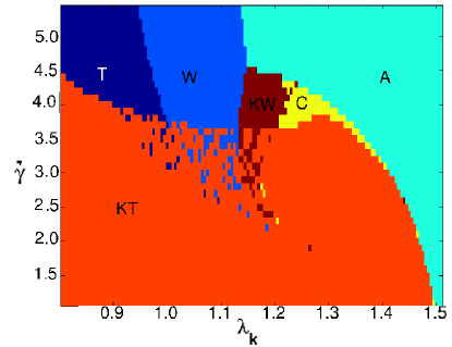
Figure 1: [Color Online] Phase diagram for dynamical behaviour in the local map defined through Eqns.II.2, with the parameter $\lambda_{k}$ plotted on the $x$ axis and $\dot{\gamma}$ on the $y$ axis. Here T denotes the tumbling state, W the wagging state, KT the kayak-tumbling, KW the kayak-wagging state, A the aligned state and C the state in which complex dynamics is seen. These states are discussed further in the text.

The states in this phase diagram are labeled as follows: The first is the state labeled $A$, which is the Aligned state, where all dynamics ceases, and the director is aligned at an angle to the flow. In the standard Couette geometry, the velocity field and the velocity gradient form a plane, called the vorticity plane. In our case, this is the $x-y$ plane. If the director lies in the vorticity plane and rotates about an axis (the $z-$axis) perpendicular to this plane, the dynamical state is called a Tumbling state. The tumbling state is denoted by $T$ in the phase diagram of Fig. (1). If the director, while lying in the plane, executes oscillations, the dynamical state is called a Wagging state. The wagging state is represented in the local phase diagram by the symbol $W$.

If the director rotates and oscillates, moving out of the vorticity plane, the dynamical states are called Kayak-Tumbling and Kayak-Wagging respectively. They are represented as KT and KW in the local phase diagram. If the dynamics is a mixture of complex intermittent behaviour and coexisting attractors, the state is called Complex and is represented by $C$ in the phase diagram. Clearly the interesting region in the phase diagram lies in and near the region labeled C.

Fig. 1 is obtained in the following way. The phase-space of the $\dot{\gamma}$ and $\lambda_{k}$ variables is gridded and an initial random initial condition chosen at each point. After the passage of an initial transient state, the system goes to dynamical attractors, ranging from simple spatiotemporal fixed points to complex intermittent behaviour. These dynamical attractors are identified with one of the states described above, i.e. $A,K,T,KW,KT$ or $C$. In some regimes, one sees a coexistence of states i.e. KT and T and KW and W i.e. different initial conditions can give rise to different asymptotic behaviour in the long time limit.

III Coupled Maps for Nematodynamics

Our spatially coupled model is built up from the local maps given in Eq. II.2. These maps are placed on the sites of a regular lattice in one and two dimensions and can be coupled via several different coupling schemes, as described below. The generalization to arbitrary dimensions as well as different coupling schemes is a straightforward one.

For a one dimensional lattice, with sites indexed by the label $i$, the five variables ($a_{0}(i)\dots a_{4}(i)$) on each lattice site evolve in discrete time $t$ as:

$$\phi_{i}=\phi^{\prime}_{i}+\frac{1}{3}\epsilon\,\big{(}\phi^{t}_{i+1}+\phi^{t}_{i-1}-2\phi^{t}_{i}\big{)},$$ (7)

where $\phi\in(a^{t+1}_{0},\,a_{1}^{t+1},\,a^{t+1}_{2},\,a_{3}^{t+1},\,a_{4}^{t+1})$ and $\phi^{\prime}\in(f_{0}(a_{0}^{t}),f_{1}(a_{1}^{t}),f_{2}(a_{2}^{t}),f_{3}(a_{3}^{t}),f_{4}(a_{4}^{t}))\;.Here\epsilon$ is a coupling constant which is chosen to take values between $0$ and $3/2$.

For the two dimensional case we consider a square lattice with site index $(i,j)$   and with the set of five variables $(a_{0}(i,j),\;a_{1}(i,j),\;a_{2}(i,j),\;a_{3}(i,j),\;a_{4}(i,j))$ on each lattice point at time-step $t$ evolving in time as :

$$\phi_{i,j} =\phi^{\prime}_{i,j} +\frac{1}{6}\epsilon\,\big{(}\phi^{t}_{i+1,j}+\phi^{t}_{i-1,j}+\phi^{t}_{i,j+1}+\phi^{t}_{i,j-1}\big{)}$$ (8)

$$+\frac{1}{12}\epsilon\,\big{(}\phi^{t}_{i+1,j+1}+\phi^{t}_{i-1,j-1}+\phi^{t}_{i-1,j+1}+\phi^{t}_{i+1,j-1}\big{)}-\epsilon\phi^{t}_{i,j},$$

where $\phi\in(a^{t+1}_{0},\,a_{1}^{t+1},\,a^{t+1}_{2},\,a_{3}^{t+1},\,a_{4}^{t+1})$ and $\phi^{\prime}\in(f_{0}(a_{0}^{t}),f_{1}(a_{1}^{t}),f_{2}(a_{2}^{t}),f_{3}(a_{3}^{t}),f_{4}(a_{4}^{t}))\;,$ and $\epsilon$ is a coupling constant having value between $0$ and $1$. The choice of the numerical coefficients $1/6$ and $1/12$ in the coefficients of the nearest and next-nearest neighbour terms are standard choices in the CML literature. They represent choices of lattice discretization which are as close as possible to the continuum limit.

The local value of the shear stress $(\sigma_{xy})_{i,j}$ at the (two-dimensional) site $(i,j)$ is obtained from the following definitionfootnote1 :

$$(\sigma_{xy})_{i,j} =(\sigma^{\prime}_{xy})_{i,j} +\frac{\sqrt{2}}{6}\epsilon\,\big{(}\phi_{i+1,j}+\phi_{i-1,j}+\phi_{i,j+1}+\phi_{i,j-1}\big{)}$$ (9)

$$+\frac{\sqrt{2}}{12}\epsilon\,\big{(}\phi_{i+1,j+1}+\phi_{i-1,j-1}+\phi_{i-1,j+1}+\phi_{i+1,j-1}\big{)}-\sqrt{2}\epsilon\phi_{i,j},$$

where $(\sigma^{\prime}_{xy})_{i,j}$ is given by

$$(\sigma^{\prime}_{xy})_{i,j}=(2\sqrt{2}a_{2}a^{2}-6\sqrt{6}(a_{3}a_{4}/2-(a_{2}a_{0}/\sqrt{3})))_{i,j},$$ (10)

and $\phi=a_{2}$.

The definition for the one-dimensional case follows from:

$$(\sigma_{xy})_{i} =(\sigma^{\prime}_{xy})_{i} +\frac{\sqrt{2}}{3}\epsilon\,\big{(}\phi_{i+1}+\phi_{i-1}-2\phi_{i}\big{)},$$ (11)

where $(\sigma^{\prime}_{xy})_{i}$ is given by

$$(\sigma^{\prime}_{xy})_{i}=(2\sqrt{2}a_{2}a^{2}-6\sqrt{6}(a_{3}a_{4}/2-(a_{2}a_{0}/\sqrt{3})))_{i},$$ (12)

and $\phi=a_{2}$.

We have also experimented with other choices of the update rule. While the update rule of Eq. 7 can be termed as the post-update rule, in which the terms on the right hand side are calculated at time $t+1$, one could alternatively use the pre-update rule, in which these terms are calculated at time $t$. We have checked that varying this choice of update rule does not affect our results. In the equation for the two-dimensional update, (Eq. 8), we have checked that dropping the next-nearest neighbour term also does not affect our results significantly. Thus, a variety of possible update schemes appear to yield consistent results for the spatio-temporal behaviour of our coupled map lattice, underlining the generic nature of our results.

In the sections below we describe the relevant features emerging from the simulation of the coupled map lattice above for a wide range of parameters and initial states.

IV The One-dimensional Coupled Map Lattice

In this section, we describe our results for the one-dimensional case, concentrating on the effects of the inter-site coupling, both within and outside the regime labelled C in the phase diagram.

IV.1 Local dynamics

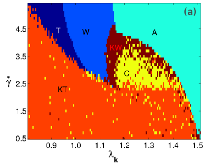
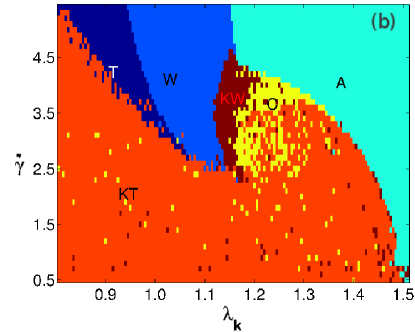
Figure 2: [Color Online] Phase diagram summarizing the local dynamical behaviour of the spatially coupled one-dimensional system, with $\lambda_{k}$ plotted on the $x$ axis and $\dot{\gamma}$ on the $y$ axis. As before, T denotes the tumbling state, W the wagging state, KT the kayak-tumbling, KW the kayak-wagging state, A the aligned state and C the state of complex dynamics. The spatial coupling constant $\epsilon=0.1$ (a) and 0.5 (b), for a ring of 200 lattice points. The location of the states in the phase diagram is largely similar to that of Fig. 1 with the exception that, at isolated points, mainly within the KT phase, one sees complex behaviour. The regime in the phase diagram occupied by the C phase shrinks as the coupling constant $\epsilon$ is increased.

Fig. (2) shows the dynamical phases exhibited by a generic site randomly chosen from the one dimensional ring. The sites are coupled according to the scheme given in Eq. 8, with coupling constant $\epsilon=0.1$ (a) and $\epsilon=0.5$ (b).

It is evident from comparisons with Fig. (1) that the local dynamics of a generic site in the coupled system is similar to the uncoupled case. This indicates that spatial coupling does not alter the nature of the local dynamics qualitatively. The most significant influence of spatial coupling occurs near the C region, which appear to be somewhat broadened with spatial coupling, while the coexistence regimes are reduced in size. In addition, the fairly uniform KT state is now “studded” with points displaying complex behaviour. This indicates coexistence of complex and KT behaviour, with certain initial states leading to complex dynamics, while others lead to a uniform KT state. (It is difficult to determine whether the complex behaviour we see is a very long transient or true asymptotic behaviour.) The tumbling T and wagging W regions, however, are very stable.

IV.1.1 Local behaviour of regular regions

Figs. (3)-(4) show the value of the scalar order parameter $s_{1}$, the biaxiality parameter $s_{2}$ and the $z$ component of the director ${\bf n}$. Fig. (3) is obtained using parameter values appropriate to the T and W regions of the local phase diagram, with a coupling constant $\epsilon=0.1$. This displays completely regular behaviour, with these quantities varying periodically keeping the director in the vorticity plane. Fig. (4) is obtained using parameter values appropriate to the KT and KW regions of the local phase diagram and indicate that the director can now fluctuate out of plane whereas all quantities vary smoothly and periodically.

Figure (5) shows the local time period with which these quantities fluctuate as a function of $\dot{\gamma}$ at $\lambda_{k}=0.9$. The time period is inversely proportional to shear rate, as is evident from the fit to the data points.

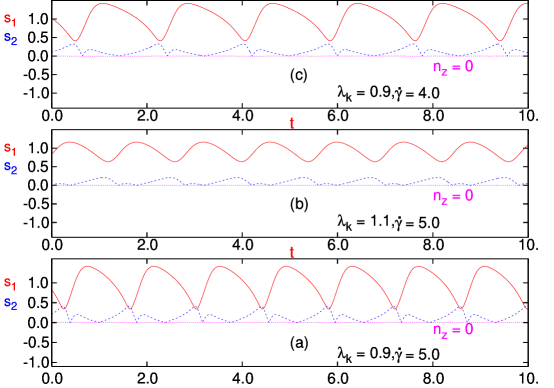
Figure 3: [Color Online] Local dynamics in a ring of 200 lattice points, with coupling $\epsilon=0.1$, showing the temporal evolution of $s_{1}$, $s_{2}$ and $n_{z}$. These are displayed for (a) $s_{1}$ ,$s_{2}$ and $n_{z}$ with (a) $\lambda_{k}=0.9$ and $\dot{\gamma}=5.0$ (b) $\lambda_{k}=1.1$ and $\dot{\gamma}=5.0$, and (c) $\lambda_{k}=0.9$ and $\dot{\gamma}=4.0$. These states are all drawn from the T and W parts of the local phase diagram. Note that $n_{z}=0$ in all these states whereas $s_{1}$ and $s_{2}$ are periodic functions of time.

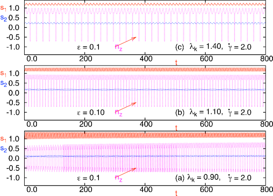
Figure 4: [Color Online] Local dynamics in a ring of 200 lattice points, with coupling $\epsilon=0.1$, showing the temporal evolution of $s_{1}$, $s_{2}$ and $n_{z}$. These are displayed for for (a) $\lambda_{k}=0.9$ and $\dot{\gamma}=2.0$ (b) $\lambda_{k}=1.1$ and $\dot{\gamma}=2.0$, and (c) $\lambda_{k}=1.4$ and $\dot{\gamma}=2.0$. These points are drawn from the KT and KW part of the local phase diagram and represent states in which the director exhibits out-of-plane fluctuations i.e. $n_{z}\neq 0$. However, $s_{1}$ and $s_{2}$ continue to exhibit regular, periodic oscillations.

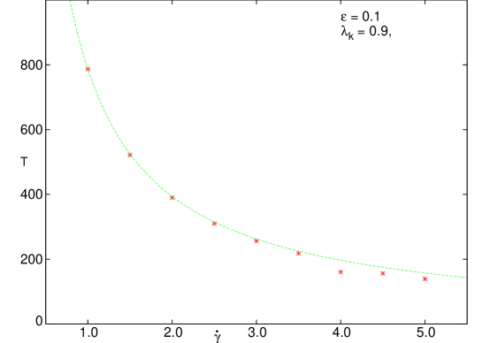
Figure 5: [Color Online] Time Period (T) vs. $\dot{\gamma}$, for the case of a ring of 200 lattice points, with coupling $\epsilon=0.1$ and with $\dot{\gamma}$ varying across the T and KT regions of the phase diagram. The numerical results are represented as points and the fitted curve is: $T\sim\frac{1}{\dot{\gamma}}$.

IV.1.2 Local Dynamics in the Complex Region

The local behaviour in the complex region, denoted by $C$ in the local phase diagram, is exhibited in Fig. (6), which shows $s_{1}$ and $s_{2}$ and $n_{z}$. The results suggest that the sites display intermittent behaviour. These results are obtained for parameter values at the boundary of the complex region and the kayak-wagging region, with paramters $\dot{\gamma}=4.0$ and $\lambda_{k}=1.2$. In part (a), the coupling constant $\epsilon$= $0.5$, in part (b) $\epsilon=0.15$ and in part (c) $\epsilon=0.1$. All of these show qualitatively similar temporally intermittent behaviour.

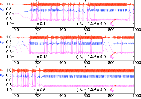
Figure 6: [Color Online] Local dynamics of a ring of 200 lattice points, with $\lambda_{k}=1.2$ and $\dot{\gamma}=4.0$, showing the time evolution of $s_{1}$, $s_{2}$ and $n_{z}$. These are shown for (a) $\epsilon=0.5$ (b) $\epsilon=0.15$ and (c) $\epsilon=0.1$, illustrating behaviour in the complex or C regime. Note that regular time-periodic behaviour is favoured at large values of the spatial coupling constant $\epsilon$, following an initial transient.

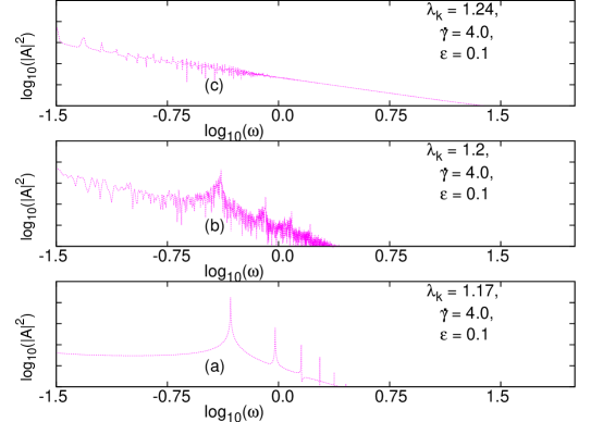
Figure 7: [Color Online] Log-Log plot of the Fourier transform vs. frequency, for (a) $\lambda_{k}=1.17$, (b) $\lambda_{k}=1.20$ and (c) $\lambda_{k}=1.24$. Here $\epsilon=0.1$ and $\dot{\gamma}=4.0$. The lattice is a ring of $200$ sites. Note that for $\lambda_{k}=1.17$ (the wagging region), the regular oscillations show up as a delta function in the fourier transform. In the C or complex region, a smooth distribution of frequencies is seen, with a $1/f^{2}$ falloff.

The fourier transform of the time series of stress calculated at a generic site and plotted on a doubly logarithmic scale is shown in Fig. (7). The spectrum in (c) of Fig. (7) fits the relation $P(f)\sim 1/f^{2}$.

IV.2 Spatio-temporal coherence and dynamics

In order to quantify the degree of spatial coherence, we calculate the following quantity for the one-dimensional lattice:

$$\overline{d}=\sqrt{\frac{1}{NT}\sum_{t=1}^{T}\sum_{i=1}^{N}(a_{0}^{t}(i)-\overline{a}^{t})^{2}},$$ (13)

where

$$\overline{a^{t}}=\frac{1}{N}\sum_{i=1}^{N}a^{t}_{0}(i).$$ (14)

We have calculate such a spatial coherence parameter for one specific component of the vector $(a_{0},\ldots,a_{4})$; however, qualitatively similar results are obtained for other components as well as for the full local stress, in the C region. When $\overline{d}$ tends to zero the degree of synchronization of the local variables is very high. On the other hand large $\overline{d}$ indicates low spatial synchronization, arising from a wide distribution of values of the local variables in the lattice. This quantity thus serves as a global order parameter characterizing the smoothness of the spatial patterns exhibited by the evolution of the map.

Fig. (8) shows the time average of the deviation $<\overline{d}>$ of $a_{0}$ from the average value $a_{0}$. To compute this, we first calculate the instantaneous deviation $\overline{d}$ via Eqs. (14) and (13), and then find the long-time average of this quantity. The spatial profile of the regular region with low $<\overline{d}>$ is characterised either by spatiotemporal fixed behaviour with all sites aligned, or spatial uniformity and temporal periodicity. There are also cases in the regular region where the sites, though not completely synchronized in space, are nevertheless phase synchronized.

IV.2.1 Spatio-temporal dynamics in the regular region

Fig. (9) displays the space-time plot for $\dot{\gamma}=4$, $\lambda_{k}=1.1$ and coupling constant $\epsilon=0.1$ (a) and $0.5$ (b). The $x$-axis displays the lattice index and time is shown on $y$-axis, increasing from top to bottom. The profile is not spatially uniform and periodic in time for very weak coupling. As the coupling is increased, the system acquires spatial coherence and temporal periodicity.

IV.2.2 Spatio-temporal dynamics in the complex region

The spatiotemporal behaviour of a representative case in the C or complex region is displayed in Fig. (10), where $\dot{\gamma}=4$, $\lambda_{k}=1.17$ and coupling constant $\epsilon$ = 0.1 (a) and 0.5 (b). It is evident that the space-time profile splits into bands, i.e. clusters of synchronized sites, where the local dynamics is either fixed (blue) or time-periodic (stripes). As we increase $\lambda_{k}$ (with $\dot{\gamma}=4$) in Figs.  (10 -  12) the length scale of the spatio-temporally intermittent pattern increases, finally yielding to the aligned region. This progression from frozen localized kinks/domains of fixed points in the spatial background of time-periodic behaviour, to infective bursts bearing the signature of spatiotemporal intermittency, is seen in many systems crutchfieldkaneko , and often arises from a competition of fixed point patterns and time-periodic and quasi-periodic patterns.

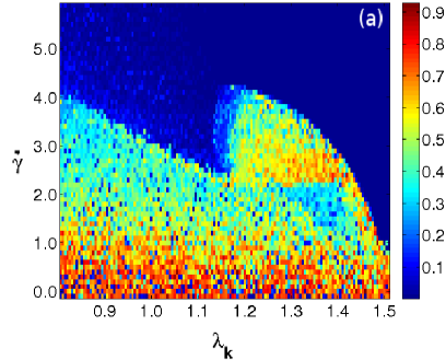
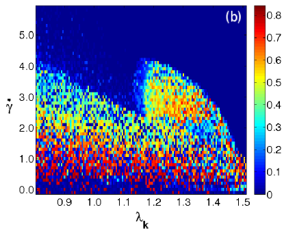
Figure 8: [Color Online] Average deviation from the mean value for $\epsilon=0.1$ (a) and $\epsilon=0.5$ (b), with $\lambda_{k}$ on the $x$-axis and $\dot{\gamma}$ on the $y$ axis. Note that large fluctuations (roughness) are seen in the KW and C regions. These data are for the 1-d system wiith the number of sites $N=200$ and parameters as indicated on the figure.

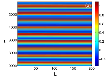
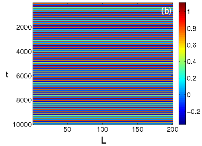
Figure 9: [Color Online] Density plot of order parameter part of shear stress. Here $\lambda_{k}$ = 1.1, $\dot{\gamma}$ =4.0 and $\epsilon$ = 0.1 (a) and 0.5 (b). Time steps (running from top to bottom) are on the $y$-axis, and the lattice site index ($i=1,200$) is on the $x$-axis. These figures represent space-uniform and time-periodic states, obtained using parameter values corresponding to the T region of the phase diagram.

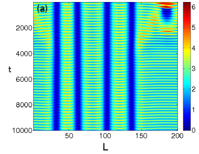
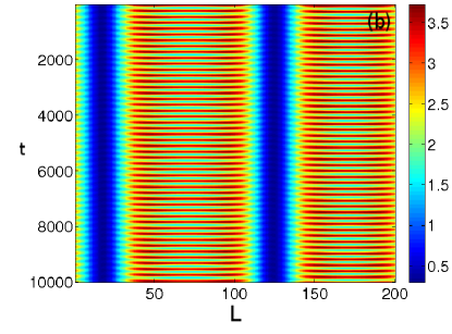
Figure 10: [Color Online] Density plot of order parameter part of shear stress. Here $\lambda_{k}$ = 1.17, $\dot{\gamma}$ =4.0 and $\epsilon$ = 0.1 (a) and 0.5 (b). Time steps (running from top to bottom) are on the $y$-axis, and the lattice site index ($i=1,200$) is on the $x$-axis. These figures represent space non-uniform and time-periodic states, obtained using parameter values corresponding to the KW region of the phase diagram

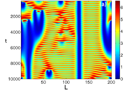
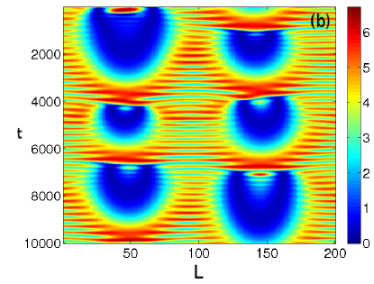
Figure 11: [Color Online] Density plot of order parameter part of shear stress. Here $\lambda_{k}$ = 1.20, $\dot{\gamma}$ =4.0 and $\epsilon$ = 0.1 (left) and 0.5 (right). Time steps (running from top to bottom) are on the $y$-axis, and the lattice site index ($i=1,200$) is on the $x$-axis. These figures illustrate how time-periodic regions are interspersed with domains of fixed point behaviour, reminiscent of spatiotemporal intermittency. The parameter values corresponding to the C region of the phase diagram, in a regime where the chaos is weak.

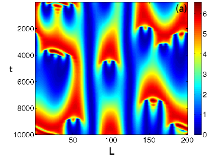
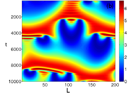
Figure 12: [Color Online] Density plot of order parameter part of shear stress. Here $\lambda_{k}$ = 1.24, $\dot{\gamma}$ =4.0 and $\epsilon$ = 0.1 (a) and 0.5 (b). Time steps (running from top to bottom) are on the $y$-axis, and the lattice site index ($i=1,200$) is on the $x$-axis. These figures illustrate non-uniform, time-varying states characteristic of spatio-temporally chaotic behaviour. The parameter values correspond to the C region of the phase diagram, in a regime where the chaos is strong. Note that larger values of $\epsilon$ lead to larger and more uniform spatial structures.

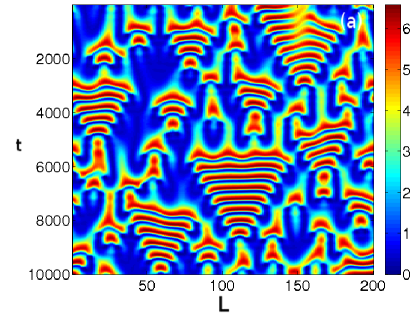
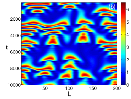
Figure 13: [Color Online] Density plot of order parameter part of shear stress. Here $\lambda_{k}$ = 1.24, $\dot{\gamma}$ =3.0 and $\epsilon$ = 0.1 (a) and 0.5 (b). Time steps (running from top to bottom) are on the $y$-axis, and the lattice site index ($i=1,200$) is on the $x$-axis.

V The Two-dimensional Coupled Map Lattice

V.1 Local temporal behaviour

We have also explored the dynamics on a two-dimensional lattice. In the regular regions of the phase diagram, corresponding to the T,W, KT and KW states, the temporal behavior is very similar to that of the one dimensional case and is thus not shown separately. We thus concentrate on behavior in the complex or C region.

Representative data showing the local temporal dynamics of the complex region is given in Fig (14). They show chaotic behaviour, and there appears to be no qualitative difference between the one dimensional and two dimensional lattice cases. As in the one-dimensional lattice, increased coupling strengths suppress the chaotic region. The log-log plot of the fourier transform is shown in Fig. (15); a similar fit to $P(f)\sim f^{-2}$ of the frequency spectrum of the stress can be obtained, as in the one-dimensional case.

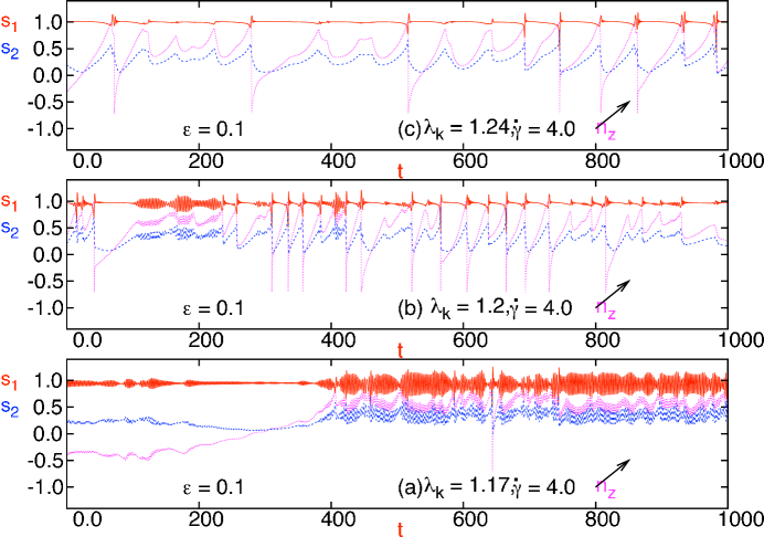
Figure 14: [Color Online] Temporal evolution of $s_{1}$, $s_{2}$ and $n_{z}$ in a two dimensional lattice of size $102\times 102$, with $\epsilon=0.1$, for (a) $\lambda_{k}=1.17$ and $\dot{\gamma}=4.0$ (b) $\lambda_{k}=1.20$ and $\dot{\gamma}=4.0$ (c) $\lambda_{k}=1.24$ and $\dot{\gamma}=4.0$. All these state points are drawn from the C region of the local phase diagram. Note the existence of temporally intermittent behavior, analysed in terms of its frequency spectrum in Fig. 15.

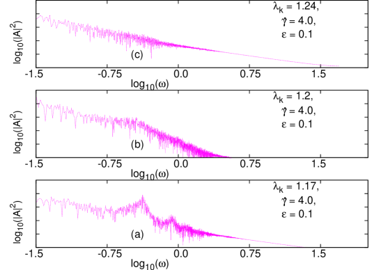
Figure 15: [Color Online] Log-Log plot of the absolute value of the Fourier transform of the stress vs. frequency $\omega$, for (a) $\lambda_{k}=1.17$, (b) $\lambda_{k}=1.20$ and (c) $\lambda_{k}=1.24$. Here $\epsilon=0.1$ and $\dot{\gamma}=4.0$. The lattice contains $100\times 100$ sites. Note the relatively smooth background, indicating the presence of a continuous set of frequencies. The fall-off is consistent with a $1/\omega^{2}$ behaviour.

V.2 Spatio-temporal behaviour

To quantify the degree of spatial coherence in $2$-dimensional lattices we calculate the quantity, generalizing from the one-dimensional case studied in an earlier section:

$$\overline{d}=\sqrt{\frac{1}{N_{1}N_{2}T}\sum_{t=1}^{T}\sum_{i,j=1}^{N1,N2}(a_{0}^{t}(i,j)-\overline{a}^{t})^{2}},$$ (15)

with

$$\overline{a}=\frac{1}{N_{1}N_{2}}\sum_{i,j=1}^{N_{1},N_{2}}a_{0}(i,j).$$ (16)

Again, as in the $1$-dimensional case, when $\overline{d}$ tends to zero the degree of synchronization of the local variables is very high. On the other hand large $\overline{d}$ indicates low spatial synchronization, and arises from a wide distribution of values of the local variables in the lattice.

Fig. (16) shows the space-time average of the deviation defined in Eqn. (15). The left panel (a) displays results for $\epsilon=0.1$ and the right panel (b) for $\epsilon=0.5$. It is clear that higher coupling strengths make the system more uniform in space. Also, it appears that the regions with kayak-tumbling, kayak-wagging and complex local dynamical behaviour show more deviation in the spatial profile, exhibiting more spatial inhomogeneity.

V.2.1 Regular regime

In this section we discuss the spatial profile of our coupled map lattice in two dimensions. As in the one-dimensional case, we start with random initial conditions and analyze the space profile after omitting a transient regime. We analyse the density plots of the shear stress contribution to the order parameter, in different dynamical regions. Considering the space-time behaviour of the system in the regular region, with local dynamics belonging to the aligned, wagging, tumbling and kayak-tumbling region, reveals spatially uniformity states which are periodicity in time. These are closely related to the states obtained in the oine-dimensional case and are not discussed further here, as we will concentrate on results obtained in the physically more interesting C regime.

V.2.2 Complex regime

The configurations in Figs. (17) and (18) are from the complex region. When the coupling becomes very large, one obtains spatially uniform states, as clear from Figs.  (17) and( 18). In Fig. 19, we have chosen points (a) and (b) from the KT region of the local phase diagram and (c) from the C dynamical region. After leaving $10^{4}$ transient steps , we have plotted one row of a $100\times 100$ lattice at a single time instant. On the $x$ axis we plot $\epsilon$ and on the $y$ axis we plot the stress at $100$ points of the lattice at one time step. It is evident that for high coupling strength $\epsilon$, the system goes to a space-synchronized state. For low coupling constants, on the other hand, there is a typically wide distribution of stress values at different sites, indicating spatial inhomogeneity.

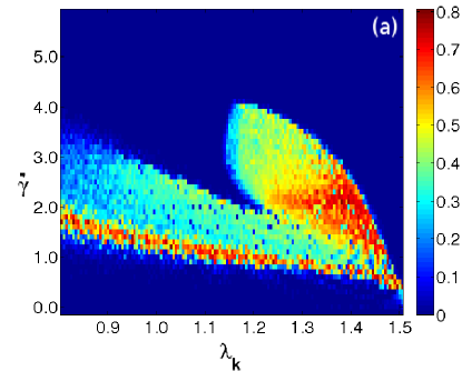
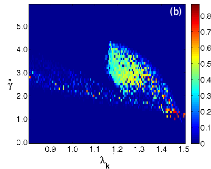
Figure 16: [Color Online] Average deviation $\overline{d}$ (see text) from the mean value of $a_{0}$ for $\epsilon$ = 0.1(right) and $\epsilon$ = 0.5(left). The quantity $\lambda_{k}$ is plotted on the $x$-axis and $\dot{\gamma}$on the $y$-axis. The lattice is a $100\times 100$-site lattice. Note that this roughness is largest in the KT, KW and C regions, especially for large values of $\dot{\gamma}$. As $\epsilon$ is increased, the roughness decreases, as increasing spatial homogeneity is promoted.

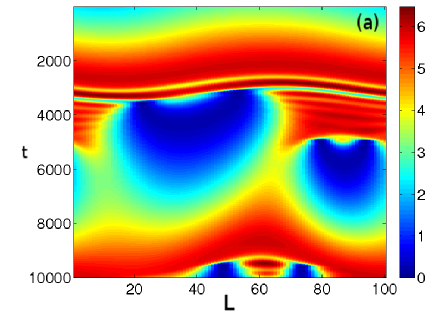
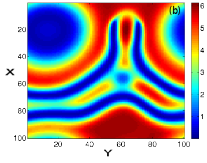
Figure 17: [Color Online] (a) A color plot of order parameter part of shear stress. The quantities $\lambda_{k}$ = 1.25, $\dot{\gamma}$ =4.0 and $\epsilon=0.1$. The time $t$ is plotted on the y-axis, which depicts the time evolution of the stress computed on one row (x-axis) of the 100 $\times$ 100 lattice. (b) shows a snap shot of the full lattice at an intermediate time step.

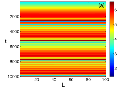
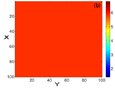
Figure 18: [Color Online] (a) A color plot of order parameter part of shear stress. The quantities $\lambda_{k}$ = 1.25, $\dot{\gamma}$ =4.0 and $\epsilon=0.5$. The time $t$ is plotted on the y-axis, which depicts the time evolution of the stress computed on one row (x-axis) of the 100 $\times$ 100 lattice. (b) shows a snap shot of the full lattice at an intermediate time step. Note that increased spatial coupling favours the space uniform time-periodic state.

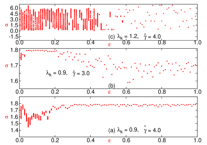
Figure 19: [Color Online] Value of stress of one row of the lattice at one instant of time on the $y$ axis as a function of the coupling strength $\epsilon$ on the $x$ axis. Note that the broad spectrum of local stress values seen at small values of the coupling contract to an essentially unique value at large $\epsilon$.

VI Quantifying Spatio-Temporal Complexity

In this section, we report results which quantify the spatio-temporal complexity in the one-dimensional coupled map lattice specified in Eq. II.2. To understand the nature of the complex behaviour represented in the phase diagram, we perform calculations of the spectrum of Lyapunov exponents, as shown in Fig. 20.

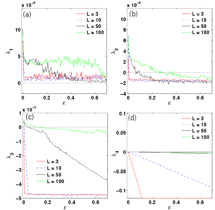
Figure 20: [Color Online] Plots of the Lyapunov exponents obtained from our calculation (see text) for different system sizes as a function of the coupling constant. The figures represent (a) he first Lyapunov exponent $\lambda_{1}$ (b) the second Lyapunov exponent $\lambda_{2}$ c) the third Lyapunov exponent $\lambda_{3}$ d) the fourth Lyapunov exponent $\lambda_{4}$. Note that all these exponents tend to zero in the limit of large system sizes and that increasing the coupling between sites has the effect of reducing the Lyapunov exponent if it were initially positive at zero coupling and increasing it, if it were initially negative.

We first choose several values of the parameters $\lambda_{k}$ and $\dot{\gamma}$ within the complex region and evolve the coupled map. After waiting for an initial number of time steps to eliminate transients, we calculate the Jacobian matrix at each time step. We then consider a small deviation from the attractor and iteratively multiply this deviation by the Jacobian, orthonormalizing this vector at each time step. From this we calculate the Lyapunov exponent, using the method described in Ref. lakshmanan .

These results are illustrated in Fig. 20, which exhibits the values of the first four Lyapunov exponents, computed for parameter values $\lambda_{k}$ and $\dot{\gamma}$ for system sizes $L=3,10,50$ and $100$, as a function of the coupling constant $\epsilon$. As can be seen from these figures, our results are the following. Qualitatively, in the complex regime, the first Lyapunov exponent is always positive, even as the system size and the spatial coupling are increased. The local value of this exponent is also positive. This value decreases further with spatial coupling but remains positive. Roughly speaking, larger lattice sizes show larger values for this exponent, consistent with results from the one-dimensional PDE calculation. These values appear to saturate for small coupling values but decrease for larger values of the spatial coupling.

The second and higher order Lyapunov exponents, in our calculation, are small and negative for the smallest lattice sizes, but move to values that are close to zero as the lattice size is increased. At small couplings, for the larger lattices, this value is positive but goes negative as the coupling strength is increased. Thus, the data for the Lyapunov exponents are consistent with the general conclusion that going to larger lattice sizes stabilizes chaos, whereas increasing the coupling between sites suppresses complex spatial behaviour. The clustering of Lyapunov exponents around zero in the large system size limit is consistent with the emergence of spatio-temporal intermittency on large scales chate1993 ; anantha ; neelima .

VII Conclusions

In summary, this paper reports a study of a coupled map lattice model constructed to study spatio-temporal aspects of rheological chaos in sheared nematic solutions. Our study was based on the construction of a suitable local map capable of reproducing the physics of the spatially uncoupled (equivalently, uniform) limit, including the variety of phases and the complex phase diagram obtained for that case. When such maps are placed on a regular (one or two-dimensional) lattice and coupled diffusively through a variety of coupling schemes, the local dynamics in the coupled map shares close similarities with the map describing the spatially uncoupled case.

Our studies of the coupled map in both one and two dimensions indicates that regimes of regular behaviour largely exhibit space-uniform and time-periodic states, with the coupled dynamics roughly following the uncoupled case. We have analysed the dynamical behaviour of the two quantities which characterize local order in the nematic, the uniaxial $s_{1}$ and the biaxial $s_{2}$ order parameters, examining their time evolution in the different states.

In contrast, in the complex or $C$ region of the local phase diagram, such coupling leads to states that exhibit spatio-temporal intermittency and chaos. We have characterized such states by examining the Lyapunov spectra as well as the frequency dependence of the time series of physical quantities such as the stress. We find evidence for a broad, power-law distribution of time-scales in the problem. Further, in the complex region, one often sees a coexistence of regular (lamina) and chaotic regimes as a prelude to fully developed chaos in which dynamical fluctuations occur independently from site to site. In some regimes, periodic bands immersed in a more complex, fluctuating background are obtained, suggestive of the possibility of transient shear bands stabilized by the dynamics, a feature also present in ODE-based studies of this problemsr ; sr1 ; debarshini . The basic scale of these complex dynamical patterns is alterable by changing the coupling constant, indicative of self-similarity in the spatio-temporally intermittent case. At very large values of the coupling constant, the space profile is expected to become uniform; however, for small and intermediate values of this coupling constant, the spectrum of Lyapunov exponents merges to zero, consistent with our observation of generic spatio-temporal intermittency in the weak coupling case.

We have experimented with using spatial coupling terms which represent the advective effects of the shear flow, coupled to fixed boundary conditions where the orientation and magnitude of the order parameter are fixed at the boundary. Such terms appear, at small amplitude, to mainly distort the sorts of dynamical structures obtained for the symmetric coupling state and seem to evolve smoothly from them.

The usefulness of coupled map lattice representations of the spatio-temporal dynamics of systems exhibiting chaos in their local dynamics is that such representations often provide both useful physical insights as well as are computationally easier to simulate than their PDE versions. In that sense, the problem of rheochaos in sheared nematics offers an ideal setting for CML methods, since the local dynamics of the sheared nematic is highly non-trivial, exhibiting a variety of temporally periodic as well as chaotic states. As shown here, the variety of non-trivial spatio-temporal behaviour exhibited by sheared nematics is very largely a consequence of simply coupling these dynamical degrees of freedom in space. The physics appears substantially independent of how precisely this spatial coupling is done, with the simple lattice model with parallel update exhibiting virtually all the behaviour of the more complex and computationally intensive studies of the appropriate PDE’s. This, together with the specific results presented in this paper for our coupled map approach to rheochaos in sheared nematics, is our central conclusion.

Further, order-parameter-based models, such as the one described in this paper and in the work of Refs. debarshini ; sr ; sr1 , contain essential non-linear terms in the free energy. It is these terms that are responsible for the non-trivial local dynamics captured in our local map as well as in the coupled map lattice. Ref. debarshini emphasizes the role of “additional complex collective dynamics” arising from such nonlinearities which is not captured in the DLS model but is relevant to the qualitative nature of the intermittent and chaotic behaviour seen in this system. Such non-linearities are naturally accounted for in our approach.

Our study of the spatio-temporal dynamics of sheared nematics using CML methods possibly represents the first extension of such methods to the problem of rheochaos. In contrast to previous work based on ODE’s which studied only the one-dimensional case, it is relatively easy to extend our CML methodology to higher dimensions, even to the experimentally relevant three-dimensional case. It would be interesting to see how, if at all, hydrodynamic effects can be incorporated in models of this type. Whether other experimental systems of sheared complex fluids which exhibiting rheochaos can be fruitfully analysed using similar coupled map approaches remains to be seen.

- (1) R. G. Larson, The Structure and Rheology of Complex Fluids, (Oxford University Press, Oxford, 1999).
- (2) M. E. Cates, in Slow Relaxations and Nonequilibrium Dynamics in Condensed Matter, Les Houches Session LXXVII, edited by J.-L. Barrat, M. Feigelman, J. Kurchan, and J. Dalibard (Springer, New York, 2003).
- (3) C. R. Safinya, E. B. Sirota, and R. J. Plano, Phys. Rev. Lett. 66, 1986 (1991).
- (4) O. Diat, D. Roux and F. Nallet, J. Phys. II France, 3 1427 (1993).
- (5) H. Yanase, P. Moldenaers, J. Mewis, V. Abetz, J. W. van Egmond, and G. G. Fuller, Rheol. Acta 30, 89 (1991).
- (6) K. Migler, C. H. Liu, and D. J. Pine, Macromolecules 29, 1422 (1996)
- (7) R. Bandyopadhyay, G. Basappa and A. K. Sood, Phys. Rev. Lett.84 2022,(2000);
- (8) R. Bandyopadhyay, G. Basappa and A. K. Sood, Pramana 53, 223(1999)
- (9) R. Bandyopadhyay, G. Basappa and A. K. Sood, Europhys. Lett. 56, 447(2001)
- (10) R. Ganapathy and A.K. Sood, Langmuir 22, 1016 (2006); Phys. Rev. Lett. 96, 108301 (2006).
- (11) P. E. Cladis and W. Van Saarloos, Solitons in Liquid Crystals, (Springer, New York, 1992) pp 136-137
- (12) N. A. Spenley, M. E. Cates, and T. C. B. McLeish, Phys. Rev. Lett. 71, 939 (1993)
- (13) M. E. Cates, T. C. B. McLeish, and G. Marrucci, Europhys. Lett. 21, 451 (1993)
- (14) N. A. Spenley, X. F. Yuan, and M. E. Cates, J. Phys. II (France) 6, 551 (1996)
- (15) P. Olmsted and C.-Y. D. Lu, Phys. Rev. E 56, R55 (1997)
- (16) P. D. Olmsted, Rheol Acta 47 283 (2008)
- (17) S. M. Fielding, Soft Matter 3 1262 (2007).
- (18) J. F. D. Berret, C. Roux and G. Porte, J. Phys. II (Paris) 4 1261 (1994)
- (19) L. B. Chen, M. K. Chow, B. J. Ackerson and C. F. Zukoski, Langmuir 10 2817 (1994)
- (20) J. F. B. Berret, C. Roux and P. Lindner, Eur. Phys. J. B 5 67 (1995)
- (21) P. Boltenhagen, Y. Hu, E. F. Matthys and D. J. Pine, Phys. Rev. Lett. 79 2359 (1997)
- (22) W. K. Wheeler, P. Fischer and G. Fuller, J. Non-Newtonian Mech. 75 193 (1998)
- (23) G. Schmidt, S. Miller, C. Schmidt and W. Richtering, Rheol. Acta 38 486 (1999)
- (24) E. Eiser, F. Morino, G. Porte and X. Pithon, Rheol. Acta 39 201 (2000)
- (25) L. Soubiran, E. Staples, I. Tucker, J. Penfold and A. Creeth, Langmuir 17 7988 (2001)
- (26) J. B. Salmon, A. Colin and D. Roux Phys. Rev. E 66, 031505 (2002)
- (27) B. Chakrabarti, M. Das, C. Dasgupta, S. Ramaswamy and A.K. Sood, Phys. Rev. Lett. 92 055501 (2004)
- (28) M. Das, B. Chakrabarti, C. Dasgupta, S. Ramaswamy and A.K. Sood, Phys. Rev. E 71 021707 (2005)
- (29) S. Hess, Z. Naturfor. 31A, 1034 (1976).
- (30) M. Doi, J. Polym. Sci. Polym. Phys. Ed., 19 229 (1981)
- (31) M. Doi and S. F. Edwards, The Theory of Polymer Dynamics, (Oxford University Press, London, 1986)
- (32) S. M. Fielding and P. D. Olmsted, Phys. Rev. Lett. 92 084502 (2004)
- (33) A. Aradian and M. E. Cates, Phys. Rev. E 73, 041508 (2006)
- (34) S. M. Fielding and P. D. Olmsted, Phys. Rev. Lett. 96 104502 (2006)
- (35) D. Chakraborty, C. Dasgupta and A.K. Sood, arXiv:1002.0213
- (36) Y. Oono and S. Puri, Physical Review A 38, 434 (1998)
- (37) K. Kaneko, Theory and Application of Coupled Map Lattices, John Wiley, Chichster (1993).
- (38) G. Reinacker, M. roger and S. Hess, Phys. Rev. E 66, 040702 (2002)
- (39) G. Rienacker, M. roger and S. Hess, Physica A 315 537 (2002)
- (40) A. W. Lees and S. F. Edwards, J. Phys. A 5, 1921 (1972).
- (41) We have explored alternative constructions for such a local map in Ref. kamil , where we studied a quaternion representation of the local orientational degrees of freedom. Incorporating spatial coupling is, however, easiest in the version studied in this paper.
- (42) S. Hess and I. Pardowitz, Z. Naturf. 36a 554 (1981).
- (43) C. Pereira Borgmeyer and S. Hess, J. Non-Equilib. Thermodyn. 20 359 (1995)
- (44) N. Kuzuu and M. Doi, J. Phys. Soc. Jpn. 52, 3486(1983).
- (45) P. D. Olmsted and P. M. Goldbart, Phys. Rev. A 41, 4578(1990); Phys. Rev. A 46, 4966(1992).
- (46) T. Qian and P. Sheng. Phys. Rev. E 58, 7475(1998).
- (47) A. M. Sonnet and E. G. Virga, Phys. Rev. E 64, 031705 (2001).
- (48) H. Pleiner, M. Liu, and H. R. Brand, Rheol. Acta 41, 375 (2002).
- (49) H. Stark and T.C. Lubensky, Phys. Rev. E 67, 061709 (2003).
- (50) P. G. de Gennes and J. Prost, The Physics of Liquid Crystals, 2nd ed., (Clarendon Press, Oxford 1993)
- (51) M. Grosso, R. Keunings, S. Crescitelli and P.K. Maffatone, Phys. Rev. Lett. 86, 3184 (2001)
- (52) Strictly speaking, the quantity defined is proportional to the stress. In particular, it is multiplied by an overall multiplicative factor involving ; see Eqn. A.1 of Ref. GR1 .
- (53) J.P. Crutchfield and K. Kaneko, in Directions in Chaos edited by Hao Bai Lin, World Scientific (Singapore, 1987) 272
- (54) M. Lakshmanan and S. Rajasekar, Nonlinear Dynamics, Springer-Verlag (2003).
- (55) H. Chate, Europhys. Lett. 21, 419 (1993)
- (56) G. Ananthakrishna and M.S. Bharathi, Phys. Rev. E 70, 026111 (2004)
- (57) Z. Jabeen and N. Gupte, Phys. Rev. E 74, 016210 (2006)
- (58) S. M. Kamil, S. Sinha and G. I. Menon, Phys. Rev. E 78 011706 (2008)