Ferromagnetism of $UGe_{2}$

Abstract

Magnetism of $UGe_{2}$ is due to the magnetic ordered moments of $5f$ uranium electrons. The strong spin-orbit coupling splits them into two groups. The magnetization is investigated in terms of two vector fields ${\bf M}_{1i}$ and ${\bf M}_{2i}$ which identify the local orientation of the magnetization of the two groups of $f$ electrons. Renormalized spin-wave theory, which accounts for the magnon-magnon interaction, and its extension are developed to describe two ferromagnetic phases in the system: low temperature large moment phase $0<T<T^{*}$ (FM2), where all $5f$ electrons contribute the ordered ferromagnetic moment, and high temperature low-moment phase $T^{*}<T<T_{C}$ (FM1), where $f$ electrons are partially ordered. Both phases are strictly ferromagnetic in accordance with experiment. The magnetization as a function of temperature is calculated. The anomalous temperature dependence of the ordered moment, known from the experiments with $UGe_{2}$, is very well reproduced theoretically. Below $T_{x}$ ($T^{*}$ in the present paper) the ferromagnetic moment increases in an anomalous way. The new understanding of the anomalous $FM2\rightarrow FM1$ transition, as a result of the magnetic order of two well separated groups of $f$ electrons, yields the key to an understanding of the ferromagnetism and transport properties in these compounds.

The uranium compound $UGe_{2}$ is a metallic ferromagnet below the Curie temperature $T_{C}=52K$ at ambient pressure with a zero temperature ordered moment $\mu_{s}=1.48\mu_{B}/U$ Onuki92 . The experimental measurements reveal the presence of an additional phase line that lies entirely within the ferromagnetic phase. The characteristic temperature of this transition $T_{x}$, which is below the Curie temperature $T_{C}$, decreases with pressure and disappears at a pressure close to the pressure at which new phase of coexistence of superconductivity and ferromagnetism emerges2fmp1 ; 2fmp2 ; 2fmp3 . The additional phase transition demonstrates itself through the change in the $T$ dependence of the ordered ferromagnetic moment2fmp5 ; 2fmp6 ; 2fmp7 . The magnetization shows an anomalous enhancement below $T_{x}$.

Magnetism of $UGe_{2}$ is due to the magnetic ordered moments of $5f$ uranium electrons. They have dual character and in $UGe_{2}$ are more itinerant than in many uranium compounds known as ”heavy-fermion systems”. The degree of delocalization of the $5f$ electrons has been explored by variety of experimental techniques. The thermodynamic properties, such as the magnetoresistance, suggest that uranium $5f$ electrons behave like $3d$ electrons in the conventional itinerant ferromagnets Onuki92 . On the other hand, the inelastic scattering experiments suggest localized character of the $5f$ electrons in $UGe_{2}$ 2fmp2 ; 2fmp3 . Finally the itinerant ferromagnetism may be inferred from the fact, that $UGe_{2}$ forms a very good metal. High quality single crystals have residual resistivity well below $1\mu\Omega cm$Pfleiderer2 .

Because of the strong spin-orbit coupling of $f$ electrons one has to label the states by the total angular momentum $\textbf{J}=\textbf{L}+\textbf{S}$, where L and S are angular and spin momenta respectively. For $f$-orbitals $l=3$ and one obtains two multiplets, an octet with $j=7/2$ and a sextet with $j=5/2$. They are well separated by the spin-orbit interaction and the energy level of the octet is higher than the sextet one. Since the number of $f$ electrons in $UGe_{2}$ is less than six, it is enough to consider $j=5/2$ sextet only.

The experiments on single crystal Oikawa indicate that UGe2 has a base-centered orthorhombic crystal structure. The sextet splits into doublet and quartet and the doublet’s energy level is lower. Then one obtains two well separated systems of $f$ electrons, which are two sources of magnetism in $UGe_{2}$. This justifies the consideration of an effective model in terms of two vector fields ${\bf M}_{1i}$ and ${\bf M}_{2i}$ which identify the local orientation of the magnetization of the different groups of $f$ electrons.

$$h_{eff} = -J_{1}\sum\limits_{\langle ij\rangle}{{\bf M}_{1i}\cdot{\bf M}_{1j}}-J_{2}\sum\limits_{\langle ij\rangle}{{\bf M}_{2i}\cdot{\bf M}_{2j}}$$ (1)

$$- J\sum\limits_{i}{{\bf M}_{1i}}\cdot{\bf M}_{2i}.$$

The exchange constants $J_{1},\,J_{2}$ and $J$ are positive (ferromagnetic), the sums are over all sites of a three-dimensional cubic lattice, and $\langle i,j\rangle$ denotes the sum over the nearest neighbors. The $LDA+U$ calculations show the existence of well separated majority spin state with orbital projection $m_{l}=0$ Pickett1 . This can be modeled with spin $1/2$ fermion and ${\bf M}_{2i}$ is the local magnetization of the itinerant electron. The saturation magnetization $"m"$ is close to $1/2$ at ambient pressure and decreases with increasing the pressure. This accounts for the fact that some sites, in the ground state, are doubly occupied or empty. The contribution of the others uranium $5f$ electrons, which occupy the lowest energy level bands, to the magnetization is described by ${\bf M}_{1i}$ vector with saturation magnetization $s=1$. One thinks of these electrons as localized, but they are not perfectly localized in $UGe_{2}$. This means that saturation magnetization $s$ could be smaller then one.

Renormalized spin-wave theory, which accounts for the magnon-magnon interaction, and its extension are developed in the present paper, to describe two ferrimagnetic phases in the system Eq.(1): low temperature phase $0<T<T^{*}$ , where $<{\bf M}_{1i}>$ and $<{\bf M}_{2i}>$ contribute the ordered ferromagnetic moment, and high temperature phase $T^{*}<T<T_{C}$, where only $<{\bf M}_{1i}>$ is nonzero. Both phases are strictly ferromagnetic.

To proceed we use the Holstein-Primakoff representation of the spin vectors ${\bf M}_{1j}(a^{+}_{j},a_{j})$ and ${\bf M}_{2j}(b^{+}_{j},\,b_{j})$, where $a^{+}_{j},\,a_{j}$ and $b^{+}_{j},\,b_{j}$ are Bose fields. One represents the Hamiltonian Eq.(1) in terms of these Bose fields keeping only the quadratic and quartic terms. The next step is to represent the Hamiltonian in the Hartree-Fock approximation $h\approx h_{HF}=h_{cl}+h_{q}$, where

$$h_{cl} = 3NJ_{1}s^{2}(u_{1}-1)^{2}+3NJ_{2}m^{2}(u_{2}-1)^{2}$$ (2)

$$+ NJsm(u-1)^{2},$$

$$h_{q} = \sum\limits_{k}\left(\varepsilon^{a}_{k}\,a_{k}^{+}a_{k}\,+\,\varepsilon^{b}_{k}\,b_{k}^{+}b_{k}\,-\,\gamma\,(a_{k}^{+}b_{k}+b_{k}^{+}a_{k})\,\right).$$

In equation (2) the wave vector $k$ runs over the first Brillouin zone of a cubic lattice, $N$ is the number of lattice’s sites, $u_{1},\,u_{2},\,u$ are the Hartree-Fock parameters, $\gamma=J\,u\,\sqrt{s\,m}$ and the dispersions are given by the equalities

$$\varepsilon^{a}_{k}=2s\,J_{1}\,u_{1}\varepsilon_{k}\,+\,m\,Ju\qquad\varepsilon^{b}_{k}=2m\,J_{2}\,u_{2}\varepsilon_{k}\,+\,s\,J\,u$$ (3)

with $\varepsilon_{k}=3-\cos k_{x}-\cos k_{y}-\cos k_{z}$. Equation (3) shows that the Hartree-Fock parameters $u_{1},\,u_{2}$ and $u$ renormalize the exchange constants $J_{1},\,J_{2}$ and $J$ respectively.

To diagonalize the Hamiltonian, one introduces new Bose fields $\alpha_{k},\,\alpha_{k}^{+},\,\beta_{k},\,\beta_{k}^{+}$,

$$a_{k}=\cos\theta_{k}\,\alpha_{k}\,+\,\sin\theta_{k}\,\beta_{k},\qquad b_{k}=-\sin\theta_{k}\,\alpha_{k}\,+\,\cos\theta_{k}\,\beta_{k}$$ (4)

with coefficients of transformation,

$$\cos\theta_{k}=\sqrt{\frac{1}{2}\,\left(1+\frac{\varepsilon^{a}_{k}-\varepsilon^{b}_{k}}{\sqrt{(\varepsilon^{a}_{k}-\varepsilon^{b}_{k})^{2}+4\gamma^{2}}}\right)},$$ (5)

and $\sin\theta_{k}=\sqrt{\left(1-\cos^{2}\theta_{k}\right)}$. The transformed Hamiltonian adopts the form

$$h_{q}=\sum\limits_{k}\left(E^{\alpha}_{k}\,\alpha_{k}^{+}\alpha_{k}\,+\,E^{\beta}_{k}\,\beta_{k}^{+}\beta_{k}\right),$$ (6)

with new dispersions

$$E^{\alpha}_{k} = \frac{1}{2}\,\left[\varepsilon^{a}_{k}+\varepsilon^{b}_{k}\,+\,\sqrt{(\varepsilon^{a}_{k}-\varepsilon^{b}_{k})^{2}+4\gamma^{2}}\right]$$

$$E^{\beta}_{k} = \frac{1}{2}\,\left[\varepsilon^{a}_{k}+\varepsilon^{b}_{k}\,-\,\sqrt{(\varepsilon^{a}_{k}-\varepsilon^{b}_{k})^{2}+4\gamma^{2}}\right]$$

With positive exchange constants $J_{1},\,J_{2},J$ and positive Hartree-Fock parameters $u_{1},\,u_{2},\,u$ the Bose fields’ dispersions are positive $\varepsilon^{a}_{k}>0,\,\,\varepsilon^{b}_{k}>0$ for all values of $k\in B$. As a result, $E^{\alpha}_{k}>0$ and $E^{\beta}_{k}\geq 0$ with $E^{\beta}_{0}=0$. Near the zero wave vector, $E^{\beta}_{k}\approx\rho k^{2}$ where $\rho$ is the spin-stiffness constant. Hence, $\beta_{k}$ is the long-range (magnon) excitation in the effective theory, while $\alpha_{k}$ is a gapped excitation.

The system of equations for the Hartree-Fock parameters have the form

$$u_{1} = 1-\frac{1}{3s}\frac{1}{N}\sum\limits_{k}\varepsilon_{k}\left[\cos^{2}\theta_{k}\,n_{k}^{\alpha}\,+\,\sin^{2}\theta_{k}\,n_{k}^{\beta}\right]$$

$$u_{2} = 1-\frac{1}{3m}\frac{1}{N}\sum\limits_{k}\varepsilon_{k}\left[\sin^{2}\theta_{k}\,n_{k}^{\alpha}\,+\,\cos^{2}\theta_{k}\,n_{k}^{\beta}\right]$$

$$u = 1-\frac{1}{N}\sum\limits_{k}\left[\left(\frac{1}{2s}\cos^{2}\theta_{k}+\frac{1}{2m}\sin^{2}\theta_{k}\right)\,n_{k}^{\alpha}\right.$$

$$+ \left.\left(\frac{1}{2m}\cos^{2}\theta_{k}+\frac{1}{2s}\sin^{2}\theta_{k}\right)\,n_{k}^{\beta}\right.$$

$$+ \left.\frac{Ju}{\sqrt{(\varepsilon^{a}_{k}\,-\,\varepsilon^{b}_{k})^{2}\,+\,4\gamma^{2}}}\,(n_{k}^{\alpha}-n_{k}^{\beta})\right]$$

where $n_{k}^{\alpha}$ and $n_{k}^{\beta}$ are the Bose functions of $\alpha_{k}$ and $\beta_{k}$ excitations. The Hartree-Fock parameters, the solution of the system of equations (Ferromagnetism of $UGe_{2}$), are positive functions of $T/J$, $u_{1}(T/J)>0,\,u_{2}(T/J)>0$ and $u(T/J)>0$. Utilizing these functions, one can calculate the spontaneous magnetization of the system, which is a sum of the spontaneous magnetization $M_{1}=<M^{z}_{1i}>$ and $M_{2}=<M^{z}_{i2}>$: $M\,=\,M_{1}\,+\,M_{2}$. In terms of the Bose functions of the $\alpha_{k}$ and $\beta_{k}$ excitations they adopt the form

$$M_{1}\,=\,s-\frac{1}{N}\sum\limits_{k}\left[\cos^{2}\theta_{k}\,n^{\alpha}_{k}\,+\,\sin^{2}\theta_{k}\,n^{\beta}_{k}\right],$$

$$M_{2}\,=\,m-\frac{1}{N}\sum\limits_{k}\left[\sin^{2}\theta_{k}\,n^{\alpha}_{k}\,+\,\cos^{2}\theta_{k}\,n^{\beta}_{k}\right],$$

$$M\,=\,s\,+\,m-\frac{1}{N}\sum\limits_{k}\left[n^{\alpha}_{k}\,+\,n^{\beta}_{k}\right].$$ (9)

Calculating the spontaneous magnetization one obtains that at characteristic temperature $T^{*}$ the spontaneous magnetization $M_{2}$ becomes equal to zero, while the spontaneous magnetization $M_{1}$ is still nonzero. This is because the magnon excitation $\beta_{k}$ in the effective theory Eq.(1) is a complicated mixture of the transversal fluctuations of the vectors ${\bf M}_{i1}$ and ${\bf M}_{i2}$ Eq.(4). As a result, the magnons’ fluctuations suppress in a different way the different magnetic orders. Above $T^{*}$ the system of equations (Ferromagnetism of $UGe_{2}$) has no solution and one has to modify the renormalized spin-wave theory.

To formulate mathematically the modified RSW theory one introduces Karchev08a two parameters $\lambda_{1}$ and $\lambda_{2}$ to enforce the two magnetic moments to be equal to zero in paramagnetic phase. To this end, we add two new terms to the effective Hamiltonian Eq.(1),

$$\hat{h}_{eff}\,=\,h_{eff}\,-\,\sum\limits_{i}\left[\lambda_{1}M^{z}_{1i}\,+\,\lambda_{2}M^{z}_{2i}\right].$$ (10)

In Hartree-Fock approximation, in momentum space, the Hamiltonian adopts the form

$$\hat{h}_{q}=\sum\limits_{k}\left(\hat{\varepsilon}^{a}_{k}\,a_{k}^{+}a_{k}\,+\,\hat{\varepsilon}^{b}_{k}\,b_{k}^{+}b_{k}\,-\,\gamma\,(a_{k}^{+}b_{k}+b_{k}^{+}a_{k})\,\right),$$ (11)

where the the new dispersions are

$$\hat{\varepsilon}^{a}_{k}\,=\varepsilon^{a}_{k}\,+\,\lambda^{l},\qquad\hat{\varepsilon}^{b}_{k}\,=\varepsilon^{b}_{k}\,+\,\lambda^{it}.$$ (12)

Utilizing the same transformation Eq.(4) with coefficients $\cos\hat{\theta}_{k}$ and $\sin\hat{\theta}_{k}$ expressed by means of $\hat{\varepsilon}^{a}_{k}$ and $\hat{\varepsilon}^{b}_{k}$ one obtains the Hamiltonian in diagonal form (6) with dispersions   $\hat{E}^{\alpha}_{k}=\hat{E}^{+}_{k}$ and $\hat{E}^{\beta}_{k}=\hat{E}^{-}_{k}$, where $\hat{E}^{\pm}_{k}=\frac{1}{2}\,\left[\hat{\varepsilon}^{a}_{k}+\hat{\varepsilon}^{b}_{k}\,\pm\,\sqrt{(\hat{\varepsilon}^{a}_{k}-\hat{\varepsilon}^{b}_{k})^{2}+4\gamma^{2}}\right]$.

It is convenient to represent the $\lambda$ parameters in the form $\lambda_{1}=mJ(\mu_{1}-1),\quad\lambda_{2}=sJ(\mu_{2}-1)$. In terms of the $\mu$ parameters the dispersions adopt the form $\hat{\varepsilon}^{a}_{k}=2sJ_{1}\,u_{1}\varepsilon_{k}+mJu\mu_{1},\quad\hat{\varepsilon}^{b}_{k}=2mJ_{2}u_{2}\varepsilon_{k}+sJu\mu_{2}$ The renormalized spin-wave theory is reproduced when $\mu_{1}=\mu_{2}=1$($\lambda_{1}=\lambda_{2}=0$). We assume $\mu_{1}$ and $\mu_{2}$ to be positive. Then, $\hat{\varepsilon}^{a}_{k}>0$, $\hat{\varepsilon}^{b}_{k}>0$, and $\hat{E}^{\alpha}_{k}>0$ for all values of the wave-vector $k$. The $\beta_{k}$ dispersion is non-negative, $\hat{E}^{\beta}_{k}\geq 0$ if $\mu_{1}\mu_{2}\geq 1$. In the particular case $\mu_{1}\mu_{2}=1$   $\hat{E}^{\beta}_{0}=0$ and near the zero wave vector $\hat{E}^{\beta}_{k}\approx\hat{\rho}k^{2}$, so $\beta_{k}$ boson is the long-range excitation (magnon) in the system. In the case $\mu_{1}\mu_{2}>1$, both $\alpha_{k}$ boson and $\beta_{k}$ boson are gapped excitations.

The parameters $\lambda_{1}$ and $\lambda_{2}$ ($\mu_{1},\mu_{2}$) are introduced to enforce the spontaneous magnetizations $M_{1}$ and $M_{2}$ to be equal to zero in the paramagnetic phase. One finds out the parameters $\mu_{1}$ and $\mu_{2}$, as well as the Hartree-Fock parameters, as functions of temperature, solving the system of five equations: equations (Ferromagnetism of $UGe_{2}$) and the equations $M_{1}=M_{2}=0$, where the spontaneous magnetizations have the same representation as equations (Ferromagnetism of $UGe_{2}$) but with coefficients $\cos\hat{\theta}_{k},\,\,\sin\hat{\theta}_{k}$, and dispersions $\hat{E}^{\alpha}_{k},\,\,\hat{E}^{\beta}_{k}$ in the expressions for the Bose functions. The numerical calculations show that for high enough temperature $\mu_{1}\mu_{2}>1$. When the temperature decreases the product $\mu_{1}\mu_{2}$ decreases, remaining larger than one. The temperature at which the product becomes equal to one ($\mu_{1}\mu_{2}=1$) is the Curie temperature.

Below $T_{C}$, the spectrum contains magnon excitations, thereupon $\mu_{1}\mu_{2}=1$. It is convenient to represent the parameters in the following way:   $\mu_{2}=\mu,\quad\mu_{1}=1/\mu$.

In the ordered phase magnon excitations are the origin of the suppression of the magnetization. Near the zero temperature their contribution is small and at zero temperature spontaneous magnetizations $M_{1}$ and $M_{2}$ reach their saturations $(M_{1}=s,\,\,M_{2}=m)$. On increasing the temperature magnon fluctuations suppress the different ordered moments in different way. At $T^{*}$ the spontaneous magnetization $M_{2}$ becomes equal to zero. Increasing the temperature above $T^{*}$, $M_{2}$ should be zero. This is why we impose the condition $M_{2}(T)=0$ if $T>T^{*}$. For temperatures above $T^{*}$, the parameter $\mu$ and the Hartree-Fock parameters are solution of a system of four equations, equations (Ferromagnetism of $UGe_{2}$) with $\cos\hat{\theta}_{k},\,\,\sin\hat{\theta}_{k},\,\,\hat{\varepsilon}_{k}^{a},\,\,\hat{\varepsilon}_{k}^{b},\,\,\hat{E}^{\alpha}_{k},\,\,\hat{E}^{\beta}_{k}$ instead of $\cos\theta_{k},\,\,\sin\theta_{k},\,\,\varepsilon_{k}^{a},\,\,\varepsilon_{k}^{b},\,\,E^{\alpha}_{k},\,\,E^{\beta}_{k}$, and the equation $M_{2}=0$. One utilizes the obtained functions $\mu(T)$, $u_{1}(T)$, $u_{2}(T)$, $u(T)$ to calculate the spontaneous magnetization as a function of the temperature. Above $T^{*}$, the magnetization of the system is equal to $M_{1}$.

The resultant magnetization-temperature curves, for different choices of the model parameters, are depicted in figure. I set the Curie temperature to be equal to the experimental one. This fixes the exchange constant $J$. The constants $J_{1}/J$ and $J_{2}/J$ are chosen so that the ratio $T_{C}/T^{*}$ to be close to the experimental value.

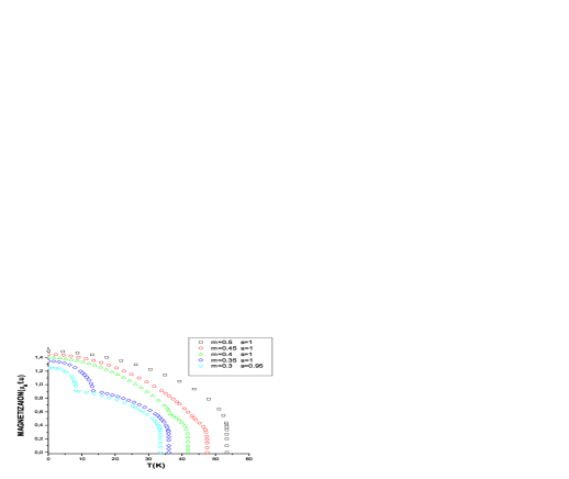
Figure 1: (color online)  Magnetization-temperature curve obtained within an effective two magnetic ordered moments model of $UGe_{2}$ magnetism

The first curve from above (black squares) is calculated for parameters $m=0.5,\,s=1,\,J_{1}/J=0.05$ and $J_{2}/J=0.0005$. The strong interaction between itinerant and ”localized” electrons aligns their magnetic orders so strong that they become zero at one and just the same temperature $T_{C}$. The magnetization-temperature curve is typical Curie-Weiss curve. The result is different if the exchange constant $J$ is relatively smaller. The ferromagnetic phase is divided into two phases: low temperature phase $0<T<T^{*}$ where $M_{1}$ and $M_{2}$ give contribution to the magnetization, and high temperature ferromagnetic phase $T^{*}<T<T_{C}$ where $M_{2}=0$. The next curve (red circles) is obtained for parameters $m=0.45,\,s=1,\,J_{1}/J=0.16,\,J_{2}/J=0.0016$, the third one (green triangles) for parameters $m=0.4,\,s=1,\,J_{1}/J=0.18$ and $J_{2}/J=0.0018$, the fourth curve (blue rhombs) corresponds to parameters $m=0.35,\,s=1,\,J_{1}/J=0.4$ and $J_{2}/J=0.004$, and for the last one $m=0.3,\,s=0.95,\,J_{1}/J=0.57$ and $J_{2}/J=0.0057$. The curves show that increasing the constants $J_{1}/J$ and $J_{2}/J$ the ration $T_{C}/T^{*}$ increases ($T_{C}/T^{*}=1,\,1.092,\,1.46,\,2.68,\,4.08$), and $T^{*}$ approaches to zero ($T^{*}=53.35K,\,43.511K,\,36.433K,\,13.44K,\,8.21K$). Comparing with experiment 2fmp3 ; 2fmp6 one concludes that increasing the pressure the exchange constant $J$ increases, but exchange constants $J_{1}$ and $J_{2}$ increase faster, so that the ratios $J_{1}/J$ and $J_{2}/J$ increase.

The anomalous temperature dependence of the ordered moment, known from the experiments with $UGe_{2}$ 2fmp2 ; 2fmp5 ; 2fmp6 ; 2fmp7 , is very well reproduced theoretically. Below $T_{x}$ ($T^{*}$ in the present paper) the ferromagnetic moment increases in an anomalous way. The low temperature, large moment phase is referred to as $FM2$, while the high temperature low-moment phase is referred to as $FM1$ 2fmp7 ; Pfleiderer2 . Both phases are strictly ferromagnetic in accordance with experiment Huxley03b . The present theoretical result gives new insight into $FM1\rightarrow FM2$ transition. It is shown that between Curie temperature and $T^{*}<T_{C}$ the contribution of the itinerant $UGe_{2}$ electrons to the magnetization is zero. They start to form magnetic moment at $T^{*}$.

There are experiments which support the present theoretical result. The measurements 2fmp5 show that the resistivity display a down-turn around $T_{C}$ and $T^{*}(=T_{x})$. The last one is best seen in terms of a broad maximum in the derivative $d\rho/dT$ Oomi1 . It is well known that the onset of magnetism in the itinerant systems is accompanied with strong anomaly in resistivity 2fmp12 . The experiments 2fmp5 ; Oomi1 prove that there are two groups of $5f$ uranium electrons. One of them starts to form magnetic order at Curie temperature, the other one does this at temperature $T_{x}(=T^{*})$ well below $T_{C}$, in agreement with the theoretical result. Further evidence for the nature of the $FM1\rightarrow FM2$ transition has been observed in the high resolution photoemission, which show the presence of a narrow peak in the density of states below $E_{F}$ that suggests itinerant ferromagnetism Ito .

In summary, it is shown that the anomalous temperature dependence of the ordered moment is a result of the splitting of $5f$ uranium electrons into two groups due to the strong spin-orbit coupling. c

It is impossible to require the theoretically calculated Curie temperature and magnetization-temperature curves to be in exact accordance with experimental results. The models are idealized, and they do not consider many important effects. Because of this it is important to formulate theoretical criteria for adequacy of the method of calculation. In my opinion the calculations should be in accordance with the Mermin-Wagner theorem M-W . It claims that at nonzero temperature, a one-dimensional or two-dimensional isotropic spin-S Heisenberg model with finite-range exchange interaction can be neither ferromagnetic nor antiferromagnetic. The renormalized spin-wave theory, developed in the present paper, being approximate captures the essentials of the magnon fluctuations and satisfies the Mermin-Wagner theorem.

This work was partly supported by a Grant-in-Aid DO02-264/18.12.08 from NSF-Bulgaria.

References

• (1) Y. $\bar{O}$nuki, I. Ukon, S.W. Yun, I. Umehara, K. Satoh, T. Fukuhara, H. Sato, S. Takayanagi, M. Shikama, and A. Ochiai, J. Phys. Soc. Jpn. 61, 293 (1992).
• (2) S. S. Saxena, P. Agarwal, K. Ahilan, F. M. Grosche, R.K.W. Haselwimmer, M.J.Steiner, E.Pugh, I.R.Walker, S. R. Julian, P. Monthoux, G. G. Lonzarich, A. Huxley, I. Sheikin, D. Braithwaite, and J. Flouquet, Nature (London) 406, 587 (2000).
• (3) A. Huxley, I. Sheikin, E. Ressouche, N. Kernavanois, D. Braithwaite, R. Calemczuk, and J. Flouquet, Phys. Rev. B 63, 144519 (2001).
• (4) N. Tateiwa, T. Kobayashi, K. Hanazono, K. Amaya, Y. Haga, R. Settai, and Y.$\bar{O}$nuki, J. Phys. Condens. Matter 13, L17 (2001).
• (5) N. Tateiwa, K. Hanazono, T. C. Kobayashi, K. Amaya, T. Inoue, K. Kindo, Y. Koike, N. Metoki, Y. Haga, R. Settai, and Y. $\bar{O}$nuki, J. Phys. Soc. Jpn 70, 2876 (2001).
• (6) C. Pfleiderer and A. D. Huxley, Phys. Rev. Lett., 89, 147005 (2002).
• (7) G. Motoyama, S. Nakamura, H. Kadoya, T. Nishioka, and N. K. Sato,Phys. Rev. B 65, 020510(R) (2001).
• (8) Christian Pfleiderer, Rev.Mod.Phys., 81, 1551 (2009).
• (9) K. Oikawa, T. Kamiyama, T. Asano, Y. Onuki, and M.Kohgi, J. Phys. Soc. Jpn, 65, 3229 (1996).
• (10) A. B. Shick and W. E. Pickett, Phys. Rev. Lett., 86, 300 (2001).
• (11) Naoum Karchev, Phys.Rev. B 77, 012405 (2008).
• (12) A. D. Huxley, V. Mineev, B. Grenier, E. Ressouche, D. Aoki, J.Flouquet, and C. Pfleiderer, J.Phys.: Condens.Matter 15, S1945, (2003).
• (13) G. Oomi, K. Kagayama, K. Nishimura, S.W. Yun, and Y. $\bar{O}$nuki, Physica B206&207, 515 (1995).
• (14) P. P. Craig, W. I. Goldburg, T. A. Kitchens, and J. I. Budnick, Phys. Rev. Lett., 19, 1334 (1967).
• (15) T. Ito, H. Kumigashira, S. Souma, T. Takahashi, Y. Haga, and Y. $\bar{O}$nuki, J. Phys. Soc. Jpn 71, Suppl.262 (2002).
• (16) S. Watanabe and K. Miyake, J. Phys. Society of Japan 71, 2489 (2002).
• (17) K. G. Sandeman, G. G. Lonzarich, and A. J. Schofield, Phys. Rev. Lett., 90, 167005 (2003).
• (18) Alexander B. Shick, Vaclav Janis, Vaclav Drchal, and Warren E. Picket, Phys. Rev. B 70, 134506 (2004).
• (19) N. D. Mermin and H. Wagner, Phys. Rev. Lett. 17, 1133 (1966).