Random polynomials and expected complexity of bisection methods for real solving

Abstract

Our probabilistic analysis sheds light to the following questions: Why do random polynomials seem to have few, and well separated real roots, on the average? Why do exact algorithms for real root isolation may perform comparatively well or even better than numerical ones?

We exploit results by Kac, and by Edelman and Kostlan in order to estimate the real root separation of degree $d$ polynomials with i.i.d. coefficients that follow two zero-mean normal distributions: for $SO(2)$ polynomials, the $i$-th coefficient has variance ${d\choose i}$, whereas for Weyl polynomials its variance is ${1/i!}$. By applying results from statistical physics, we obtain the expected (bit) complexity of sturm solver, $\widetilde{\mathcal{O}}_{B}(rd^{2}\tau)$, where $r$ is the number of real roots and $\tau$ the maximum coefficient bitsize. Our bounds are two orders of magnitude tighter than the record worst case ones. We also derive an output-sensitive bound in the worst case.

The second part of the paper shows that the expected number of real roots of a degree $d$ polynomial in the Bernstein basis is $\sqrt{2d}\pm\mathcal{O}(1)$, when the coefficients are i.i.d. variables with moderate standard deviation. Our paper concludes with experimental results which corroborate our analysis.

Categories and Subject Descriptors: F.2 [Theory of Computation]: Analysis of Algorithms and Problem Complexity; I.1 [Computing Methodology]: Symbolic and algebraic manipulation: Algorithms

Keywords: Random polynomial, real-root isolation, Bernstein polynomial, expected complexity, separation bound

1 Introduction

One of the most important procedures in computer algebra and algebraic algorithms is root isolation of univariate polynomials. The goal is to compute intervals in the real case, or squares in the complex case, that isolate the roots of the polynomial and to compute one such interval, or square, for every root.

We restrict ourselves to exact algorithms, i.e. algorithms that perform arithmetic with rational numbers of arbitrary size. The best known algorithms are subdivision algorithms, based on Sturm sequences (sturm), or on Descartes’ rule of sign (descartes), or on Descartes’ rule and the Bernstein basis representation (bernstein). Subdivision algorithms mimic binary search and their complexity depends on separation bounds. They are given an initial interval, or compute one containing all real roots. Then, they repeatedly subdivide it until it is certified that zero or one real root is contained in the tested interval.

Thanks to important recent progress [7, 8, 10, 11], the complexity of sturm, descartes and bernstein is, in the worst case, $\widetilde{\mathcal{O}}_{B}(d^{4}\tau^{2})$, where $d$ is the degree of the polynomial and $\tau$ the maximum coefficient bitsize. The bound holds even when the polynomial is non-squarefree, and we also compute (all) the multiplicities. This requires a preprocessing of complexity $\widetilde{\mathcal{O}}_{B}(d^{2}\tau)$, in order to compute the square-free factorization. The new polynomial has coefficients of size $\mathcal{O}(d+\tau)$. The complexity of this stage, although significant in practice, is asymptotically dominated. In this paper we consider the behavior of sturm on random polynomials of various forms. Our results can be extended to descartes and bernstein.

Another important exact solver (cf) is based on the continued fractions expansion of the real roots e.g. [1, 33, 35]. Several variants of this solver exist, depending on the method used to compute the partial quotients of the real roots. Assuming the Gauss-Kuzmin distribution holds for the real algebraic numbers, it was proven [35], that the expected complexity is $\widetilde{\mathcal{O}}_{B}(d^{4}\tau^{2})$. By spreading the roots, the expected complexity becomes $\widetilde{\mathcal{O}}_{B}(d^{3}\tau)$ [35]. The currently known worst-case bound is $\widetilde{\mathcal{O}}_{B}(d^{4}\tau^{2})$ [25]. This paper reduces the gap between sturm cf.

Numerical algorithms compute an approximation, up to a desired accuracy, of all complex roots. They can be turned into isolation algorithms by requiring the accuracy to be equal to the theoretical worst-case separation bound. The current record is $\widetilde{\mathcal{O}}_{B}(d^{3}\tau)$ and is achieved by recursively splitting the polynomial until one obtains linear factors that approximate sufficiently the roots [32, 27]. It seems that the bounds could be improved to $\widetilde{\mathcal{O}}_{B}(d^{2}\tau)$ with a more sophisticated splitting process. We should mention that optimal numerical algorithms are very difficult to implement.

Even though the complexity bounds of the exact algorithms are worse than those of the numerical ones, recent implementations of the former tend to be competitive, if not superior, in practice, e.g. [19, 30, 11, 35]. Our work attempts to provide an explanation for this. There is a huge amount of work concerning root isolation and the references stated represent only the tip of the iceberg; we encourage the reader to refer to the references.

Most of the work on random polynomials, which typically concerns polynomials in the monomial basis, focuses on the number of real roots. Kac’s [20] celebrated result estimated the expected number of real roots of random polynomials (named after himself) as $\frac{2}{\pi}\log{d}+\mathcal{O}(1)$, when the coefficients are standard normals i.i.d. or uniformly distributed, and $d$ is the degree of the polynomial. We refer the reader to e.g. [5, 24, 12] for a historical perspective and to [3] for various references. A geometric interpretation of this result and many generalizations appear in [9]. We mainly examine $SO(2)$ polynomials, where the $i$-th coefficient is an i.i.d. Gaussian random variable of zero mean and variance ${d\choose i}$. According to [9], they are “the most natural definition of random polynomials”, see also [34]. Their expected number of real roots is $\sqrt{d}$. For Weyl polynomials, the $i$-th coefficient is an i.i.d. Gaussian random variable of zero mean and variance ${1/i!}$, and the expected number of real roots is about $\frac{2}{\pi}\sqrt{d}+\mathcal{O}(1)$ where higher-order terms are not known to date [31]. For results on complex roots we refer to e.g. [14, 13].

Our first contribution concerns the expected bit complexity of sturm, when the input is random polynomials with i.i.d. coefficients; notice that their roots are not independently distributed! In other words, we have to go beyond the theory of Kac, and Edelman and Kostlan, in order to study the statistical behavior of root differences and, more precisely, the minimum absolute difference. We examine $SO(2)$ and Weyl random polynomials, and exploit the relevant progress achieved in statistical physics. In fact, these polynomial classes are of particular interest in statistical physics because they model zero-crossings in diffusion equations and, eventually, a chaotic spin wave-function [4, 14, 31]. The key observation is that, by applying these results, we can quantify the correlation between the roots, which is sufficiently weak, but does exist. For both classes of polynomials we prove an expected case bit complexity bound of $\widetilde{\mathcal{O}}_{B}(r\,d^{2}\tau)$, where $r$ is the number of real roots. A close related bound was speculated in [18], based on experimental evidence.

Our bounds are tighter than those of the worst case by two factors. In the course of this analysis, sturm is shown to be output-sensitive, with complexity proportional to the number of real roots in the given interval, even in the worst case. A similar bound appeared in [15].

Besides polynomials in the monomial basis, polynomials in the Bernstein basis are important in many applications, e.g. CAGD and geometric modeling. They are of the form $\sum_{i=0}^{d}{a_{i}{d\choose i}x^{i}(1-x)^{d-i}}$. For the random polynomials that we consider, $a_{i}$ are standard normals i.i.d. random variables, that is Gaussians with zero mean and variance one. Such polynomials are also important in Brownian motion [21]. In [2], they examine random polynomial systems; they also estimate the expected number of real roots of a polynomial in the Bernstein basis as $\sqrt{d}$, when the variance is ${d\choose i}$. This left open the case, see also [21], of smaller variance, that is polynomial and not exponential in $d$.

Our second contribution is to examine random polynomials in the Bernstein basis of degree $d$, with i.i.d. coefficients with mean zero and “moderate” variance $\Theta(1/\sqrt{d/(i(d-i))})$, for $d>i>0$. Indeed, we have $1\geq\sqrt{d/(i(d-i))}\geq 2/\sqrt{\pi d}$. We prove that the expected number of real roots of these polynomials is $\sqrt{2d}\pm\mathcal{O}(1)$. We conclude with experimental results which corroborate our analysis, and shows that these polynomials behave like polynomial with variance 1. This is the first step towards bounding the expected complexity of solving polynomials in the Bernstein basis.

The rest of the paper is structured as follows. First we specify our notation. Sec. 2 and 3 applies our expected-case analysis to estimating the real root separation bound, and to estimating the complexity of sturm solver. Sec. 4 determines the expected number of real roots of random polynomial in the Bernstein basis and supports our bounds by experimental results. The paper concludes with a discussion of open questions.

Notation. $\mathcal{O}_{B}$ means bit complexity and the $\widetilde{\mathcal{O}}_{B}$-notation means that we are ignoring logarithmic factors. For $A=\sum_{i=1}^{d}{a_{i}X^{i}}\in\mathsf{ZZ}[X]$, $\mathsf{dg}(A)$ denotes its degree. $\mathcal{L}\left(A\right)$ denotes an upper bound on the bitsize of the coefficients of $A$ (including a bit for the sign). For $\mathsf{a}\in\mathrm{\,\raise 1.42082pt\hbox{\scriptsize\bf(}\!\!\!Q}$, $\mathcal{L}\left(\mathsf{a}\right)\geq 1$ is the maximum bitsize of the numerator and the denominator. $\Delta$ is the separation bound of $A$, that is the smallest distance between two (real or complex, depending on the context) roots of $A$.

2 Subdivision-based solvers

In order to make the presentation self-contained, we present in some detail the general scheme of the subdivision-based solvers. The pseudo-code of a such a solver is found in Alg. 1. Our exposition follows closely [11].

The input is a square-free polynomial $A\in\mathsf{ZZ}[x]$ and an interval $\mathscr{I}_{0}$, that contains the real roots of $A$ which we wish to isolate; usually it contains all the positive real roots of $A$. In what follows, except if explicitly stated otherwise, we consider only the roots (real and/or complex) of $A$ with positive real part, since similar results could be obtained for roots with negative real part using the transformation $x\mapsto-x$. Our goal is to compute rational numbers between the real roots of $A$ in $\mathscr{I}_{0}$.

Input: Square-free $A\in\mathsf{ZZ}[x]$, $\mathscr{I}_{0}=[0,\mathsf{B}]$

Output: A list of isolating intervals for the real roots of $A$ in $\mathscr{I}_{0}$

AlgoLine0.1

$\textnormal{{initialization}}_{\textnormal{{sm}}}(A,\mathscr{\mathscr{I}}_{0})$ AlgoLine0.2

AlgoLine0.3

$L\leftarrow\emptyset,\,Q\leftarrow\emptyset$, $Q\leftarrow\textnormal{{push}}(Q,\{A,\mathscr{I}_{0}\})$ AlgoLine0.4

AlgoLine0.5

while $Q\neq\emptyset$ do  AlgoLine0.6

$\{f,\mathscr{I}\}\leftarrow\textnormal{{pop}}(Q)$AlgoLine0.7

$V\leftarrow\textnormal{{count}}_{\textnormal{{sm}}}(f,\mathscr{I})$ AlgoLine0.8

AlgoLine0.9

switch $V$ do  AlgoLine0.10

case $V=0$ continueAlgoLine0.11

case $V=1$ $L\leftarrow\textnormal{{ add}}(L,\mathscr{I})$ AlgoLine0.12

case $V>1$   $\{f_{L},\mathscr{I}_{L}\},\{f_{R},\mathscr{I}_{R}\}\leftarrow\textnormal{{split}}_{\textnormal{{sm}}}(f,\mathscr{I})$ AlgoLine0.13

$Q\leftarrow\textnormal{{push}}(Q,\{f_{L},\mathscr{I}_{L}\})$, $Q\leftarrow\textnormal{{push}}(Q,\{f_{R},\mathscr{I}_{R}\})$ AlgoLine0.14

      return $L$ AlgoLine0.15

Algorithm 1 ${\textsc{subdivisionSolver}}(A,\mathscr{I}_{0})$

15

15

15

15

15

15

15

15

15

15

15

15

15

15

15

The algorithm uses a stack $Q$ that contains pairs of the form $\{f,\mathscr{I}\}$. The semantics are that we want to isolate the real roots of $f$ contained in interval $\mathscr{I}$. ${\textsc{push}}(Q,\{f,\mathscr{I}\})$ inserts the pair $\{f,\mathscr{I}\}$ to the top of stack $Q$ and ${\textsc{pop}}(Q)$ returns the pair at the top of the stack and deletes it from $Q$. ${\textsc{add}}(L,\mathscr{I})$ inserts $\mathscr{I}$ to the list $L$ of the isolating intervals.

There are 3 sub-algorithms with index sm, which have different specializations with respect to the subdivision method applied, namely sturm, descartes, or bernstein. Generally, ${\textsc{initialization}}_{{\textsc{sm}}}$ does the necessary pre-processing, ${\textsc{count}}_{{\textsc{sm}}}(f,\mathscr{I})$ returns the number (or an upper bound) of the real roots of $f$ in $\mathscr{I}$, and ${\textsc{split}}_{{\textsc{sm}}}(f,\mathscr{I})$ splits $\mathscr{I}$ to two equal subintervals and possibly modifies $f$.

The complexity of the algorithm depends on the number of times the while-loop (Line LABEL:alg:Subdivision-while-loop of Alg. 1) is executed and on the cost of ${\textsc{count}}_{{\textsc{sm}}}(f,\mathscr{I})$ and ${\textsc{split}}_{{\textsc{sm}}}(f,\mathscr{I})$. At every step, since we split the tested interval to two equal sub-intervals, we may assume that the bitsize of the endpoints is augmented by one bit. If we assume that the endpoints of $\mathscr{I}_{0}$ have bitsize $\tau$, then at step $h$, the bitsize of the endpoints of $\mathscr{I}\subseteq\mathscr{J}_{0}$ is $\tau+h$.

Let $n$ be the number of roots with positive real part, and $r$ the number of positive real roots, so $r\leq n\leq d$. Let the roots with positive real part, be $\alpha_{j}=\Re(\alpha_{j})+\mathrm{\bf i}\,\Im(\alpha_{j})$, where $1\leq j\leq n$ and the index denotes an ordering on the real parts. Let $\Delta_{i}$ be the smallest distance between $\alpha_{i}$ and another root of $A$, and $s_{i}=\mathcal{L}\left(\Delta_{i}\right)$. Finally, let the separation bound, i.e. the smallest distance between two (possibly complex) roots of $A$ be $\Delta$ and its bitsize be $s=\mathcal{L}\left(\Delta\right)$.

2.1 Upper root bound

Before applying a subdivision-based algorithm, we should compute a bound, $\mathsf{B}$, on the (positive) roots. We will express this bound as a function of the bitsize of the separation bound and the degree of the polynomial. There are various bounds for the roots of a polynomial, e.g. [36, 16, 26], and references therein. For our analysis we use the following bound [16] on the positive real parts of the roots, $\mathsf{B}=\left\lfloor 2\max_{a_{i}<0}\min_{a_{k}>0,k>i}{\left|\frac{a_{i}}{a_{d}}\right|^{1/(k-i)}}\right\rfloor$, for which we have the estimation [16, 33] $\alpha_{r}\leq\Re(\alpha_{n})<\mathsf{B}<\frac{8d}{\ln{2}}\Re(\alpha_{n})$. The bound can be computed in $\widetilde{\mathcal{O}}_{B}(d^{2}\tau)$.

If we multiply the polynomial by $x$, then 0 is a root. By definition of $s$, we have $|\log(|\Re(\alpha_{i})-\Re(\alpha_{j})|)|\leq s$, for any $i\not=j$. Hence, we have the following inequalities

$$\begin{array}[]{rclcrr}\Re(\alpha_{1})&-&0&\leq&2^{s}\\ \Re(\alpha_{2})&-&\Re(\alpha_{1})&\leq&2^{s}\\ &&&\vdots&\\ \Re(\alpha_{n-1})&-&\Re(\alpha_{n-2})&\leq&2^{s}\\ \Re(\alpha_{n})&-&\Re(\alpha_{n-1})&\leq&2^{s}&(+)\\ \hline\cr&&\Re(\alpha_{n})&\leq&n\,2^{s}\end{array}$$

Thus, we have $\mathsf{B}<\frac{8d}{\ln{2}}\Re(\alpha_{n})<\frac{8d}{\ln{2}}n2^{s}<16\,d^{2}\,2^{s}<d^{2}\,2^{4+s}$. Hence, we can deduce that $\mathcal{L}\left(\mathsf{B}\right)=\mathcal{O}(s+\lg{d})$.

Lemma 2.1

Let $A\in\mathsf{ZZ}[x]$, where $\mathsf{dg}(A)=d$ and $\mathcal{L}\left(A\right)=\tau$. We can compute a bound, $\mathsf{B}$, on the positive real parts of the roots of $A$, for which it holds $\mathsf{B}<d^{2}\,2^{4+s}$, and $\mathcal{L}\left(\mathsf{B}\right)=\mathcal{O}(s+\lg{d})$.

Remark 2.2

In the worst case, the asymptotics of, more or less, all root bounds in the literature, e.g. [36, 16, 26], are same, since $\mathsf{B}\leq\max_{i}{\mathopen{|}a_{i}\mathclose{|}}\leq 2^{\tau}$, and $\mathcal{L}\left(\mathsf{B}\right)\leq\tau$. However, it is very important in practice to have good initial bounds. Good initial estimations of the roots can speed up the implementation by 20% [22].

3 On expected complexity

Expected complexity aims to capture and quantify the property for an algorithm to be fast for most inputs and slow for some rare instances of these inputs. Let $E$ denote the set of inputs, and assume it is equipped with a probability measure $\mu$; then let $c(I)$ denote the usual worst-case complexity of the considered algorithm for input $I$. By definition, the expected complexity is the integral $\int_{E}c(I)\mu(I)$.

In our setting the set $E$ depends on a parameter $d$ (the degree of the input polynomial), and we are interested in the asymptotic expected complexity when $d$ tends to infinity. Each $E_{d}$ is equipped with a probability measure $\mu_{d}$ (also called distribution) of the sequence of the (normalized) coefficients of the input polynomial and we consider the cases where there exists a limit distribution.

3.1 Strategy and Independence

A natural strategy is to decompose $E_{d}$ into two subsets $G_{d}$ and $R_{d}$ (G stands for generic and R for rare), such that $c(I)$ is small for $I\in G_{d}$ while $\mu_{d}(I)$ is very small for $I\in R_{d}$ and moreover the two partial integrals $\int_{G_{d}}c(I)\mu_{d}(I)$ and $\int_{R_{d}}c(I)\mu_{d}(I)$ are balanced or at least both small.

We face another difficulty. Classical properties and estimates in Probability theory are often expressed for a sequence of independent variables (i.i.d.) but most natural bijective transformations performed in Computer Algebra do not respect independence. For instance, if $X$ and $Y$ are independent random variables, then $U:=X+Y$ and $V:=X-Y$ are not independent. In our setting, even if we consider a model of distribution of coefficients which assumes that they are i.i.d., then this does not imply that the roots are i.i.d. and we cannot apply usual tools or estimates. However, as we are interested in asymptotic behavior, for some models of distribution of coefficients it happens that the limit distribution of the roots behave almost like a set of independent variables, i.e. they have very weak correlation. So we can invoke general classical estimates for our analysis.

When this is not the case, a useful tool is the two-point, or multi-point, correlation function. They express the defect of independence between a set of random variables and classically serve, e.g., to compute standard deviations.

Hereafter, we restrict ourselves to models of distribution of coefficients, hence induced distribution of roots, for which the corresponding probability measures and correlation functions have already been studied. Hopefully these models will provide good approximations for the situations encountered in the many applications.

3.2 $SO(2)$ polynomials

We consider the univariate polynomial $A=\sum_{i=0}^{d}{a_{i}x^{i}}$, the coefficients of which are i.i.d. normals with mean zero and variances ${d\choose i}$, where $0\leq i\leq d$. Alternatively, we could consider $A$ as $A=\sum_{i=0}^{d}\sqrt{d\choose i}\,a_{i}\,x^{i}$, where $a_{i}$ are i.i.d. standard normals. These polynomials are considered by Edelman and Kostlan [9] to be “the more natural definition of a random polynomial”. They are called $SO(2)$ because the joint probability distribution of their zeros is $SO(2)$ invariant, after homogenization. In [31] they are called binomial. Let $\rho(t)=\frac{\sqrt{d}}{\pi(1+t^{2})}$ be the true density function, i.e. the expected number of real zeros per unit length at a point $t\in\mathrm{I\!R}$. The expected number $r$ of real roots of $A$ is given by $r=\int_{\mathrm{I\!R}}{\rho(t)dt}=\sqrt{d}$ [9]. Let $\alpha_{j}$ be the real roots of $A$ in their natural ordering, where $1\leq j\leq r$.

We define the straightened zeros of $A$ as

$$\zeta_{j}=\mathcal{P}(\alpha_{j})=\sqrt{d}\;\arctan(\alpha_{j})/\pi,\,j=1,\dots,r,$$

in bijective correspondence with the real roots $\alpha_{j}$ of the random polynomial, where $\mathcal{P}(t)=\int_{0}^{t}{\rho(u)\;du}$. Moreover, the ordering is preserved. The straightened zeros are uniformly distributed on the circle of length $2\sqrt{d}$ [4, sec.5]. This is a strong property and implies that the joint probability distribution density function of two, resp. $m$, (distinct) straightened zeros coincides with their 2-point, resp. $m$-point, correlation function [4].

Proposition 3.1

[4, Thm. 5.1] Following the previous notation, as $d\rightarrow\infty$ the limit 2-point correlation of the straightened zeros is $k(s_{1},s_{2})\rightarrow\pi^{2}|s_{1}-s_{2}|/4$, when $s_{1}-s_{2}\rightarrow 0$.

Let $\Delta(\alpha)=\min_{1\leq i<r}\{\alpha_{i+1}-\alpha_{i}\}$ and $\Delta(\zeta)=\min_{1\leq i<r}\{\zeta_{i+1}-\zeta_{i}\}$ be the separation bound of the real roots of $A$ and the straightened zeros, respectively. We consider each straightened zero uniformly distributed on a straight-line interval of length $2\sqrt{d}$. For two such zeros, we can consider one horizontal and one vertical such interval, defining a square, which represents their joint probability space. Since the real roots are naturally ordered, if two of them lie in a given infinitesimal interval, they must be consecutive.

Let $Z$ be a zone bounded above and below by a diagonal at vertical distance $l$ from the main diagonal of the unit square. The probability $\operatorname{Pr}[\Delta(\zeta)\leq l]$ that there exist two zeros lying in a given interval of infinitesimal length $l$ tends to the integral of $k(s_{1},s_{2})$ over the straightened zeros lying in $Z$, as $d\rightarrow\infty$:

$$\begin{array}[]{rl}\operatorname{Pr}[\Delta(\zeta)\leq l]\rightarrow&\int_{Z}k(s_{1},s_{2})\,ds_{1}\,ds_{2}\\ =&2\int_{0}^{2\sqrt{d}}ds_{1}\,\int_{s_{1}}^{s_{1}+l}k(s_{1},s_{2})\,ds_{2}\\ =&\frac{\pi^{2}}{2}\int_{0}^{2\sqrt{d}}ds_{1}\,\int_{s_{1}}^{s_{1}+l}\mathopen{|}s_{1}-s_{2}\mathclose{|}\,ds_{2}=\frac{\pi^{2}\,\sqrt{d}}{2}\,l^{2},\end{array}$$

where the first integral is over all straightened zeros, which lie in an interval of size $2\sqrt{d}$. Notice that $k(s_{1},s_{2})$ is essentially the joint probability density function of two real roots. Using Markov’s inequality, e.g. [28] we have $\operatorname{Pr}[\Delta(\zeta)\geq l]\leq\operatorname{E}[\Delta(\zeta)]/l$, so

$$\operatorname{E}[\Delta(\zeta)]\geq l\,\operatorname{Pr}[\Delta(\zeta)\geq l]=l-l\,\operatorname{Pr}[\Delta(\zeta)<l]>l-\frac{\pi^{2}\,\sqrt{d}}{2}\,l^{3}.$$

This bounds the asymptotic expected separation conditioned on the hypothesis that it tends to zero, as $d\rightarrow\infty$. If we choose $l=1/(d^{c}\tau)$, where $c\geq 1$ is a (small) constant, which is in accordance with the assumption of $l\rightarrow 0$, then $\operatorname{E}[\Delta(\zeta)]>\tfrac{1}{d^{c}\tau}-\tfrac{\pi^{2}}{2\,d^{3c-1/2}\tau^{3}}$.

$$\operatorname{E}[\Delta(\zeta)]=\operatorname{E}[\min_{1\leq i<r}\{\zeta_{i+1}-\zeta_{i}\}]=$$

$$\frac{\sqrt{d}}{\pi}\,\operatorname{E}[\min_{1\leq i<r}\{\arctan(\alpha_{i})-\arctan(\alpha_{i+1})]=$$

$$\frac{\sqrt{d}}{\pi}\,\operatorname{E}[\min_{1\leq i<r}\{\arctan\left(\frac{\alpha_{i}-\alpha_{i+1}}{1+\alpha_{i}\,\alpha_{i+1}}\right)\}]>\frac{1}{d^{c}\tau}-\frac{\pi^{2}}{2\,d^{3c-1/2}\tau^{3}}\Leftrightarrow$$

$$\operatorname{E}[\min_{1\leq i<r}\{\arctan\left(\frac{\alpha_{i}-\alpha_{i+1}}{1+\alpha_{i}\,\alpha_{i+1}}\right)\}]>\frac{\pi}{d^{c+1/2}\tau}-\frac{\pi^{3}}{2\,d^{3c}\tau^{3}}.$$

Function $\arctan$ is strongly monotone, and $1+\alpha_{i}\alpha_{i+1}\geq 1$, for all $i$, except where $\alpha_{i}$ is the largest negative root and $\alpha_{i+1}$ is the smallest positive root. But we can treat this case separately, since zero is an obvious separation point.

$$\operatorname{E}[\min_{1\leq i<r}\{\alpha_{i}-\alpha_{i+1}\}]\geq\operatorname{E}[\min_{1\leq i<r}\{\left(\frac{\alpha_{i}-\alpha_{i+1}}{1+\alpha_{i}\,\alpha_{i+1}}\right)\}]>$$

$$>\tan(\frac{\pi}{d^{c+1/2}\tau}-\frac{\pi^{3}}{2\,d^{3c}\tau^{3}})\geq\frac{\pi}{d^{c+1/2}\tau}-\frac{\pi^{3}}{2\,d^{3c}\tau^{3}},$$

where the latter inequality follows from the series expansion $\tan x=x+x^{3}/3+\cdots$ for $x\in(0,\pi/2)$.

Lemma 3.2

Let $A\in\mathsf{ZZ}[x]$ of degree $d$, the coefficients of which are i.i.d. variables that follow a normal distribution with variances ${d\choose i}$, then for the expected value of the separation bound of the real roots it holds $\operatorname{E}[\Delta]>\frac{\pi}{d^{c+1/2}\tau}-\frac{\pi^{3}}{2\,d^{3c}\tau^{3}}$, for a constant $c\geq 1$, and $\operatorname{E}[s]=\operatorname{E}[\mathcal{L}\left(\Delta\right)]=\mathcal{O}(\lg{d}+\lg{\tau})$.

3.3 Weyl polynomials

We consider random polynomials, known as Weyl polynomials, which are of the form

$$A=\sum_{i=0}^{d}{a_{i}x^{i}/\sqrt{i!}},$$

where the coefficients $a_{i}$ are independent standard normals. Alternatively, we could consider $A$ as $A=\sum_{i=0}^{d}{a_{i}x^{i}}$, where $a_{i}$ are normals of mean zero and variance $1/\sqrt{i!}$. The density of the real roots of Weyl polynomials is

$$\rho(t)=\frac{1}{\pi}\sqrt{1+\frac{t^{2d}(t^{2}-d-1)}{e^{t^{2}}\Gamma(n+1,t^{2})}-\frac{t^{4d+2}}{(e^{t^{2}}\Gamma(n+1,t^{2}))^{2}}},$$

where $\Gamma$ is the incomplete gamma function. The expected number of real roots is $r=\int_{\mathrm{I\!R}}{\rho(t)dt}\sim\frac{2}{\pi}\sqrt{d}$ [31], where the higher order terms of the number of real roots are not explicitly known up to now.

The asymptotic density, for $d\rightarrow\infty$, is

$$\rho(t)=\begin{cases}\pi^{-1},&\mathopen{|}t\mathclose{|}\ll\sqrt{d}\\ \frac{d}{\pi t^{2}},&\mathopen{|}t\mathclose{|}\gg\sqrt{d}\end{cases}$$ (1)

A useful observation is that the density of the real roots of the Weyl polynomials is similar to the density of the real eigenvalues of Ginibre random matrices, that is $d\times d$ matrices with elements Gaussian i.i.d. random variables [9, 31].

We consider only the real zeros of $A$ that are inside the disc centered at the origin with radius $\sqrt{d}$ since outside the disc there is only a constant number of them. In this case the density is represented by the first branch of (1).

We work as in the case of the $SO(2)$ polynomials. Now $\mathcal{P}(t)=\int_{0}^{t}{\rho(u)du}=t/\pi$. The straightened zeros, $\zeta_{i}$, are given by

$$\zeta_{i}=\mathcal{P}(\alpha_{i})=\alpha_{i}/\pi,$$

and they are uniformly distributed in $[0,\sqrt{d}/\pi]$ [31]. The joint probability distribution density function of two straightened zeros coincides with their 2-point correlation function.

Proposition 3.3

[31] Under the previous notation, as $d\rightarrow\infty$ the limit 2-point correlation of the straightened zeros is $w(s_{1},s_{2})\rightarrow|s_{1}-s_{2}|/(4\pi)$, when $s_{1}-s_{2}\rightarrow 0$.

Working as in the case of the $SO(2)$ polynomials, the probability $\operatorname{Pr}[\Delta(\zeta)\leq l]$ that there exist two roots lying in a given interval of infinitesimal length $l$ tends to the integral of $w(s_{1},s_{2})$ over the straightened zeros lying in $Z$, as $d\rightarrow\infty$:

$$\begin{array}[]{rl}\operatorname{Pr}[\Delta(\zeta)\leq l]=&\int_{Z}{w(s_{1},s_{2})ds_{1}ds_{2}}\\ =&\int_{0}^{\sqrt{d}/\pi}\int_{s_{1}-l}^{s_{1}+l}w(s_{1},s_{2})\,ds_{1}\,ds_{2}=\frac{l^{2}\sqrt{d}}{4\pi^{2}},\end{array}$$

and using Markov’s inequality

$$\operatorname{Pr}[\Delta(\zeta)\geq l]\leq\operatorname{E}[\Delta(\zeta)]/l\Longleftrightarrow\operatorname{E}[\Delta]>l-\frac{\sqrt{d}}{4\pi^{2}}l^{3}.$$

If we choose $l=1/(d^{c}\tau)$, where $c\geq 1$ is a (small) constant, we get $\operatorname{E}[\Delta(\zeta)]>\frac{1}{d^{c}\tau}-\frac{1}{4\pi^{2}d^{3c-1/2}\tau^{3}}$ and $\operatorname{E}[\Delta(\alpha)]>\frac{\pi}{d^{c}\tau}-\frac{1}{4\pi d^{3c-1/2}\tau^{3}}$.

Lemma 3.4

Let $A\in\mathsf{ZZ}[x]$ of degree $d$, the coefficients of which are i.i.d. variables that follow a normal distribution with variances $1/i!$, then for the expected value of the separation bound of the real roots it holds $\operatorname{E}[\Delta]>\frac{\pi}{d^{c}\tau}-\frac{1}{4\pi d^{3c-1/2}\tau^{3}}$ and $\operatorname{E}[s]=\operatorname{E}[\mathcal{L}\left(\Delta\right)]=\mathcal{O}(\lg{d}+\lg{\tau})$.

3.4 The sturm solver

Probably the first certified subdivision-based algorithm is the algorithm by Sturm, circa 1835, based on his theorem: In order to count the number of real roots of a polynomial in an interval, one evaluates a negative polynomial remainder sequence of the polynomial and its derivative over the left endpoint of the interval and counts the number of sign variations. We do the same for the right endpoint; the difference of sign variations is the number of real roots.

We assume that the positive real roots are contained in $[0,\mathsf{B}]$ (Sec. 2.1). If there are $r$ of them, then we need to compute $r-1$ separating points. The magnitude of the separation points is at most $\frac{1}{2}\Delta_{j}$, for $1\leq j\leq r$, and to compute each we need $\left\lceil\lg{\frac{2\,\mathsf{B}}{\Delta_{j}}}\right\rceil$ subdivisions, performing binary search in the initial interval. Let $T$ be the binary tree that corresponds to the execution of the algorithm and $\#(T)$ be the number of its nodes, or in other words the total number of subdivisions:

$$\#(T)=\sum_{j=1}^{r}{\left\lceil\lg{\frac{2\mathsf{B}}{\Delta_{j}}}\right\rceil}\leq 2r+r\lg{\mathsf{B}}-\sum_{j=1}^{r}{\lg{\Delta_{j}}}.$$ (2)

Using Lem. 2.1, we deduce that $\#(T)=\mathcal{O}(rs+r\lg(d))$.

The Sturm sequence should be evaluated over a rational number, the bitsize of which is at most the bitsize of the separation bound. Using fast algorithms [23, 29] this cost is $\widetilde{\mathcal{O}}_{B}(d^{2}(\tau+s))$; to derive the overall complexity we should multiply it by $\#(T)$. Notice that for the evaluation we use the sequence of the quotients, which we computed in $\widetilde{\mathcal{O}}_{B}(d^{2}\tau)$ [23, 29], and not the whole Sturm sequence, which can be computed in $\widetilde{\mathcal{O}}_{B}(d^{3}\tau)$, e.g. [7].

The previous discussion allows us to express the bit complexity of sturm not only as a function of the degree and the bitsize, but also using the number of real roots and the (logarithm of) separation bound. This complexity is output sensitive, and is of independent interest, although it leads to a loose worst-case bound.

Lemma 3.5

Let $A\in\mathsf{ZZ}[x]$, $\mathsf{dg}(A)=d$, $\mathcal{L}\left(A\right)=\tau$ and let $s$ be the bitsize of its separation bound. Using sturm, we isolate the real roots of $A$ with worst-case complexity $\widetilde{\mathcal{O}}_{B}(rd^{2}(s^{2}+\tau s))$, where $r$ is the number of real roots.

In the worst case $s=\mathcal{O}(d\tau)$, and to derive the worst case complexity bound for sturm, $\widetilde{\mathcal{O}}_{B}(d^{4}\tau^{2})$, we should also take into account that $ds=\mathcal{O}(d\tau)$.

To derive the expected complexity we should consider two cases for the separation bound, that is, smaller or bigger than $l=1/(d^{c}\tau)$, where $c\geq 1$ is a small constant that shall be specified later.

In the first case, that is $\Delta\leq l=1/(d^{c}\tau)$, the real roots are not well separated, so we rely on the worst case bound for isolating them, that is $\widetilde{\mathcal{O}}_{B}(d^{4}\tau^{2})$. This occurs with probability $\operatorname{Pr}[\Delta\leq l]=\Theta(\sqrt{d}\,l^{2})=\Theta(\frac{1}{d^{2c-1/2}\,\tau^{2}})$, by the computations of Sec. 3.2 and Sec.3.3. This probability is very small.

For the second case, since $\Delta>1/(d^{c}\tau)$ we deduce $s=\mathcal{O}(lg{d}+\lg{\tau})$. The complexity of isolating the real roots, following Lem. 3.5 is $\widetilde{\mathcal{O}}_{B}(rd^{2}\tau)$. The computations in Sec. 3.2 and Sec.3.3 suggest that this case occurs with probability $\operatorname{Pr}[\Delta>l]=1-\Theta(\sqrt{d}\,l^{2})=1-\Theta(\frac{1}{d^{2c-1/2}\,\tau^{2}})$, which is close to one.

The expected-case complexity bound of sturm is

$$\widetilde{\mathcal{O}}_{B}\left((1-\frac{1}{d^{2c-1/2}\,\tau^{2}})\cdot rd^{2}\tau+\frac{1}{d^{2c-1/2}\,\tau^{2}}\cdot d^{4}\tau^{2}\right)=\widetilde{\mathcal{O}}_{B}(rd^{2}\tau),$$

for any $c\geq 1$, by using $\sqrt{d}=\widetilde{\mathcal{O}}(r\tau)$, which follows from the expected number of real roots. To avoid using this expected number, it suffices to set $c\geq 2$.

Theorem 3.6

Let $A\in\mathsf{ZZ}[x]$, where $\mathsf{dg}(A)=d$, $\mathcal{L}\left(A\right)=\tau$. If $A$ is either a $SO(2)$ or a Weyl random polynomial, then the expected complexity of sturm solver is $\widetilde{\mathcal{O}}_{B}(r\,d^{2}\tau)$.

In practice, the Sturm sequence is used and not the quotient sequence. The cost of the former is $\widetilde{\mathcal{O}}_{B}(d^{3}\tau)$ which dominates the bound of Th. 3.6. This explains the empirical observations that most of the execution time of sturm solver is spend on the construction of the Sturm sequence.

4 Random Bernstein polynomials

We compute the expected number of real roots of polynomials with random coefficients, represented in the Bernstein basis. We start with some lemmata.

Lemma 4.1

For $k\leq n$, non-negative integers, it holds

$$\sum\limits_{j=0}^{n}{{k\,n\choose k\,j}x^{k\,j}}=\frac{1}{k}\,\sum_{j=0}^{k-1}{(x+{e}^{\mathrm{\bf i}\frac{2\,\pi\,j}{k}})^{k\,n}}.$$

• We consider the RHS of the equality. For a specific $j$ we expand the summand, and get terms of the form

  $${k\,n\choose\mu}\,x^{kn-\mu}\,e^{\mathrm{\bf i}\frac{2\,\pi\,j}{k}\mu},\;0\leq\mu\leq kn.$$

  There are $kn+1$ such terms. Recall that $e^{\mathrm{\bf i}\,2\pi}=1$. Let $\mu=\lambda k+\nu$, where $1\leq\nu\leq k-1$, $0\leq\lambda<n$, then

  $${nk\choose\lambda k+\nu}\,x^{kn-\lambda k-\nu}\,e^{\mathrm{\bf i}\frac{2\,\pi\,j}{k}(\lambda k+\nu)}={nk\choose\lambda k+\nu}\,x^{kn-\lambda k-\nu}\,e^{\mathrm{\bf i}\frac{2\,\pi\,j}{k}\lambda k}\,e^{\mathrm{\bf i}\frac{2\,\pi\,j}{k}\nu}={nk\choose\lambda k+\nu}\,x^{kn-\lambda k-\nu}\,e^{\mathrm{\bf i}\frac{2\,\pi\,j}{k}\nu}.$$

  If we sum all these terms over $j$, we get

  $$\sum_{j=0}^{k-1}{{nk\choose\lambda k+\nu}\,x^{kn-\lambda k-\nu}\,e^{\mathrm{\bf i}\frac{2\,\pi\,j}{k}\nu}}={nk\choose\lambda k+\nu}\,x^{kn-\lambda k-\nu}\,\sum_{j=0}^{k-1}{e^{\mathrm{\bf i}\frac{2\,\pi\,j}{k}\nu}}=0,$$

  since $\sum_{j=0}^{k-1}{e^{\mathrm{\bf i}\frac{2\,\pi\,j}{k}}}=0$.

  Let $\mu=\lambda k$. In this case, we have

  $${nk\choose\lambda k}\,x^{kn-\lambda k}\,e^{\mathrm{\bf i}\frac{2\,\pi\,j}{k}\lambda k}={nk\choose\lambda k}\,x^{kn-\lambda k}={nk\choose k(n-\lambda)}\,x^{k(n-\lambda)}$$

  Notice that $0\leq\lambda\leq n$. Summing up over all $\lambda$ and all $j$, and multiplying by $1/k$ we get the LHS.  ${\square}$

Lemma 4.2

For non-negative integers $n,k,p$,

$$\frac{{n\choose k}^{p}}{{pn\choose pk}}\approx\sqrt{p\left(\frac{n}{2\pi}\right)^{p-1}}\,\sqrt{\left(\frac{1}{k(n-k)}\right)^{p-1}}.$$

• The proof follows easily from Stirling’s approximation $n!\approx\sqrt{2\pi n}\,(\frac{n}{e})^{n}$.  ${\square}$

More accurate results could be obtained if the more precise expression $\sqrt{2\pi n}\,(\frac{n}{e})^{n}\,e^{\frac{1}{12n+1}}<n!<\sqrt{2\pi n}\,(\frac{n}{e})^{n}\,e^{\frac{1}{12n}}$, is considered.

4.1 The expected number of real roots

We aim to count the real positive roots of a random polynomial in the Bernstein basis of degree $d$, i.e.

$$\widehat{P}:=\sum_{k=0}^{k=d}b_{k}{d\choose k}z^{k}(1-z)^{d-k},$$ (3)

where we assume that $\widehat{P}(0)\widehat{P}(1)\not=0$, and $\{b_{k}\}$ is an array of random real numbers, following the normal distribution, with “moderate” standard deviation, which shall be specified below.

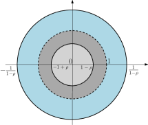
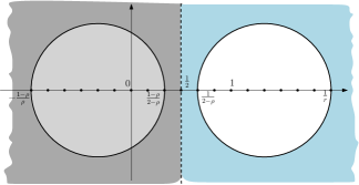
Figure 1: The transformation $z:=\frac{y}{y+1}$ in $\mathbb{C}$.

We introduce a suitable change of coordinates, $z:=y/(y+1)$, to transform a polynomial in the Bernstein basis into one in the monomial basis, by setting $P=(1+y)^{d}\widehat{P}(y)$. Now, $P$ and $\widehat{P}$ have the same number of real roots, and

$$P=\sum_{k=0}^{k=d}b_{k}{d\choose k}y^{k}.$$

Even though the number of real roots does not change, their distribution over the real axis does, see Fig. 1. In particular, we can now apply the techniques already used by Edelman, Kostlan, and others for counting the number (and, eventually, the limit distribution) of real roots. Of course, by symmetry, the expected number of positive and negative real roots is equal.

By Lem. 4.2, setting $p=2$ and $n=d$ we deduce:

$${d\choose k}\approx\sqrt{\sqrt{\frac{d}{\pi}}\,\sqrt{\frac{1}{k(d-k)}}}\sqrt{{2d\choose 2k}}=:\sqrt{S_{k}}\,\sqrt{{2d\choose 2k}}.$$ (4)

It holds that $\sqrt{2/{\sqrt{\pi d}}}\leq{{d\choose k}}/{\sqrt{{2d\choose 2k}}}=\sqrt{S_{k}}\leq 1$. To prove this, notice that $S_{k}$ is decreasing from 1 to $d/2$ and increasing from $d/2$ to $d-1$. Hence the lower bound is attained at $k=d/2$ and the upper bound at $k=1$ and $k=d-1$.

Since $S_{k}$ is small compared to ${d\choose k}$, it is reasonable to assume that omitting it will make only a negligible change in the asymptotic analysis.

Let $y=x^{2}$, with $x>0$. Now the problem at hand to count the positive real roots of

$$P=\sum_{k=0}^{k=d}{a_{k}\sqrt{{2d\choose 2k}}x^{2k}}.$$

We need the following proposition

Proposition 4.3

[9] Let $v(t)=(f_{o}(t),\dots,f_{n}(t))^{\top}$ be a vector of differentiable functions and $c_{0},\dots,c_{n}$ elements of a multivariate normal distribution with zero mean and covariance matrix $C$. The expected number of real zeros on an interval (or a measurable set) $I$ of the equation $c_{0}f_{0}(t)+\cdots+c_{n}f_{n}(t)=0$, is

$$\int_{I}{\frac{1}{\pi}\mathopen{\|}\mathbf{w}^{\prime}(t)\mathclose{\|}dt},\;\mathbf{w}=w(t)/\mathopen{\|}w(t)\mathclose{\|}.$$

where $w(t)=C^{1/2}v(t)$. In logarithmic derivative notation, this is

$$\frac{1}{\pi}\int_{I}{\sqrt{\frac{\partial^{2}}{\partial x\partial y}\log{(v(x)^{\top}Cv(x)})|_{x=y=t}}dt}.$$

For computing the integral in Prop. 4.3, we shall use the logarithmic derivative notation. Following Prop. 4.3, $f_{2i}(t)=\sqrt{{2d\choose 2i}}x^{2i}$ and $f_{2i+1}(t)=0$, $c_{2i}=a_{i}$ and $c_{2i+1}=0$, where $0\leq i\leq d$, and the variance is 1. Then,

$$v(x)^{\top}Cv(y)=\sum_{k=0}^{d}{2d\choose 2k}(xy)^{2k}.$$

We consider function

$$f(z)=\sum_{k=0}^{d}{2d\choose 2k}z^{2k}.$$

By Lem. 4.1, for $k=2$, we have $f(z)=\frac{1}{2}\left((1+z)^{2d}+(1-z)^{2d}\right)$ and so $f^{{}^{\prime}}(z)=d(z+1)^{2d-1}+d(z-1)^{2d-1}$, $f^{{}^{\prime\prime}}(z)=d(2d-1)(z+1)^{2d-2}+d(2d-1)(z-1)^{2d}$.

The following quantities are also relevant $ff^{{}^{\prime}}=\frac{1}{2}d(z+1)^{4d-1}+dz(z^{2}-1)^{2d-1}+\frac{1}{2}(z-1)^{4d-1}$, $ff^{{}^{\prime\prime}}=\frac{1}{2}d(2d-1)(z+1)^{4d-2}+d(2d-1)(z^{2}+1)(z^{2}-1)^{2d-2}+\frac{1}{2}(2d-1)(z-1)^{4d-2}$, and $(f^{\prime})^{2}=d^{2}(z+1)^{4d-2}+2d^{2}(z^{2}-1)^{2d-1}+d^{2}(z-1)^{4d-2}$.

It holds that

$$\partial_{x}\partial_{y}(\log f(x,y))=\frac{f^{{}^{\prime}}f+xyf^{{}^{\prime\prime}}f-xy(f^{{}^{\prime}})^{2}}{f^{2}}=\frac{A}{f^{2}},$$

with

$$\begin{array}[]{rl}A=&d(z+1)^{4d-2}(\frac{1}{2}(z+1)+\frac{1}{2}(2d-1)z-zd)\\ &+d(z^{2}-1)^{2d-2}(z(z^{2}-1)+(2d-1)z(z^{2}+1)-2d(z^{2}-1)z)\\ &-d(z-1)^{4d-2}(\frac{1}{2}(z-1)+\frac{1}{2}(2d-1)z-zd)\\ =&\frac{1}{2}d\left((z+1)^{4d-2}+4(2d-1)z(z^{2}-1)^{2d-2}-(z-1)^{4d-2}\right).\end{array}$$

If we let $z=t^{2}$, then

$$\begin{array}[]{ll}\frac{A(t^{2})}{f(t^{2})^{2}}&=\frac{\frac{1}{2}d((1+t^{2})^{4d-2}+4(2d-1)t^{2}(t^{4}-1)^{2d-2}-(t^{2}-1)^{4d-2})}{\frac{1}{4}((1+t^{2})^{2d}+(1-t^{2})^{2d})^{2}}\\ &=2d\frac{1}{(1+t^{2})^{2}}\frac{1+(2d-1)\left(\frac{2t}{1+t^{2}}\right)^{2}\left(\frac{1-t^{2}}{1+t^{2}}\right)^{2d-2}-\left(\frac{1-t^{2}}{1+t^{2}}\right)^{4d-2}}{\left(1+\left(\frac{1-t^{2}}{1+t^{2}}\right)^{2d}\right)^{2}}.\end{array}$$

We consider the substitutions $t=\tan\frac{\theta}{2}$, $\tan\theta=\frac{2t}{1-t^{2}}$, $\sin\theta=\frac{2t}{1+t^{2}}$, $\cos\theta=\frac{1-t^{2}}{1-t^{2}}$, and $\frac{d\theta}{2}=\frac{dt}{1+t^{2}}$. Then

$$\begin{array}[]{l}\frac{A}{f(t^{2})^{2}}=2d\frac{1}{(1+t^{2})^{2}}\frac{1+(2d-1)\sin^{2}{\theta}(\cos{\theta})^{2d-2}-(\cos{\theta})^{4d-2}}{\left(1+(\cos{\theta})^{2d}\right)^{2}}.\end{array}$$

The expected number of positive real roots is given by

$$\begin{array}[]{lll}I&=&\frac{1}{\pi}\int_{0}^{\infty}{\frac{\sqrt{A}}{f(t^{2})}}dt\\ &=&\frac{1}{\pi}\int_{0}^{\pi}{\sqrt{2d}\frac{\sqrt{1+(2d-1)\sin^{2}\theta(\cos\theta)^{2d-2}-(\cos\theta)^{4d-2}}}{1+(\cos\theta)^{2d}}}\frac{d\theta}{2}.\end{array}$$

Performing the change $\theta\mapsto\pi-\theta$, we notice that $I$ equals twice the integral between $0$ and $\pi/2$. Hence, the expected number of positive real roots of $P$ in $(0,1)$ equals that in $(1,\infty)$. Hence,

$$\begin{array}[]{l}I=\frac{\sqrt{2d}}{\pi}\int_{0}^{\pi/2}{\frac{\sqrt{1+(2d-1)\sin^{2}\theta(\cos\theta)^{2d-2}-(\cos\theta)^{4d-2}}}{1+(\cos\theta)^{2d}}}d\theta.\end{array}$$

Now we will bound the integral as $d\rightarrow\infty$. Applying the triangular inequality and noticing that $1+(cos\theta)^{4d-2}\leq 1$ and $a+\cos{\theta}^{2d}\geq 1$, we get

$$\begin{array}[]{lcl}I&\leq&\frac{\sqrt{2d}}{\pi}\left[\int_{0}^{\pi/2}{\sqrt{1}\,d\theta}+\int_{0}^{\pi/2}{\sqrt{2d-1}\sin{\theta}(\cos{\theta})^{d-1}\,d\theta}\right]\\ &=&\frac{\sqrt{2d}}{\pi}\left(\frac{\pi}{2}+\sqrt{2d-1}\,\frac{1}{d}\right)=\frac{\sqrt{2d}}{2}\left(1+\frac{1}{\pi}\frac{\sqrt{2d-1}}{d}\right)\\ &\leq&\frac{\sqrt{2d}}{2}\left(1+\frac{1}{\pi}\sqrt{\frac{2}{d}}\right)\leq\frac{\sqrt{2d}}{2}+\frac{1}{\pi}.\end{array}$$

For a lower bound, we neglect the positive term $(2d-1)\sin^{2}\theta(\cos\theta)^{2d-2}$, and notice that $\sqrt{1+(\cos{\theta})^{4d-2}}\geq 1+(\cos{\theta})^{2d-1}\geq 1+(\cos{\theta})^{2d-2}=(1+(\cos{\theta})^{d-1})(1-(\cos{\theta})^{d-1})$, and $\frac{1+(\cos{\theta})^{d-1}}{1+(\cos{\theta})^{2d}}\geq 1$.

Lemma 4.4

$$W(n):=\int_{0}^{\pi/2}{(\cos{\theta})^{n}\,d\theta}\leq\frac{2}{\sqrt{\pi}}\frac{1}{\sqrt{d+1}}.$$

• We need the following inequality [6] on Wallis’ cosine formula:

  $$\frac{1}{\sqrt{\pi(k+4\pi^{-1}-1)}}\leq\frac{1\cdot 3\cdot 5\cdots(2k-1)}{2\cdot 4\cdot 6\cdots(2k)}\leq\frac{1}{\sqrt{\pi(k+1/4)}}.$$

  If $n$ is even then $W(n)=\frac{\pi}{2}\frac{(n-1)!!}{n!}=\frac{\pi}{2}\frac{1\cdot 3\cdot 5\cdots(n-1)}{2\cdot 4\cdot 6\cdots(n)}\leq\frac{\pi}{\sqrt{\pi(2n+1)}}\leq\frac{2}{\sqrt{\pi}}\frac{1}{\sqrt{d+1}}$.

  If $n$ is odd then $W(n)=\frac{(n-1)!!}{n!}=\frac{2\cdot 4\cdot 6\cdots(n-3)(n-1)}{1\cdot 3\cdot 5\cdots(n-2)n}\leq\sqrt{\pi(k+4\pi^{-1}-1)}\cdot\frac{1}{n}\leq\frac{2}{\sqrt{\pi}}\frac{1}{\sqrt{d+1}}$.  ${\square}$

Using the lemma, $\int_{0}^{\pi/2}{(\cos{\theta})^{d-1}\,d\theta}\leq\frac{2}{\sqrt{\pi}}\frac{1}{\sqrt{d}}$, so:

$$\begin{array}[]{lll}I&\geq&\frac{\sqrt{2d}}{\pi}\int_{0}^{\pi/2}{1-(\cos{\theta})^{d-1}\,d\theta}\\ &\geq&\frac{\sqrt{2d}}{2}\left(1-\frac{4}{\pi\sqrt{\pi}}\frac{1}{\sqrt{d}}\right)\geq\frac{\sqrt{2d}}{2}-\sqrt{\frac{8}{\pi^{3}}}.\end{array}$$

Hence $I=\frac{\sqrt{2d}}{2}\pm\mathcal{O}(1)$ and we can state the following:

Theorem 4.5

The expected number of real roots of a random polynomial $P=\sum_{k=0}^{k=d}{a_{k}\sqrt{{2d\choose 2k}}x^{2k}}$, where $a_{k}$ are standard normals i.i.d. random variables, is $\sqrt{2d}\pm\mathcal{O}(1)$.

By employing (4) and considering $\sqrt{S_{k}}$ as part of the deviation, we have the following:

Corollary 4.6

The expected number of real roots of a random polynomial in the Bernstein basis, Eq. (3), the coefficients of which are normal i.i.d. random variables with mean 0 and variance $1/S_{k}=1/\sqrt{\frac{d}{\pi k(d-k)}}$, is $\sqrt{2d}\pm\mathcal{O}(1)$.

In Table 1 we present the results of experiments with polynomials in the Bernstein basis (see Eq. (3)), of degree $\leq 1000$, the coefficients of which are i.i.d. random variables following the standard normal distribution, that is mean zero and variance 1. For each degree we tested 100 polynomials. The first column is the degree, while the second is the expected number of real roots predicted by Cor. 4.6 which assumes variance $1/S_{k}$. The third column is the average number of real roots computed. Our experiments support the following conjecture:

Conjecture 4.7

The expected number of real roots of a random polynomial in the Bernstein basis, Eq. (3), the coefficients of which are standard normal i.i.d. random variables, that is with mean 0 and variance 1, is $\sqrt{2d}\pm\mathcal{O}(1)$.

Columns 4-7 of Tab. 1 corresponds to the average number of real roots in the intervals $(-\infty,-1)$, $(-1,0)$, $(0,1)$ and $(1,\infty)$, respectively. For these experiments we took random polynomials in the monomial basis and converted them to the Bernstein basis. The roots of a random polynomial in the monomial basis, under the assumptions of [17], concentrate around the unit circle. The symmetry of the density suggests that each of the intervals $(-1/(1-\rho),-1)$, $(-1,-1+\rho)$, $(1-\rho,1)$, and $(1,1/(1-\rho))$, contains on the average $1/4$ of the real roots (Fig. 1, left). If we apply the transformation $x\mapsto x/(x+1)$ (Fig. 1, right) to transform the polynomial to the Bernstein basis, then $3/4$ of the real roots are positive, $1/2$ of them are in $(0,1)$ and $1/4$ in $(1,\infty)$. We refer to the last columns of Tab. 1 for experimental evidences of this.

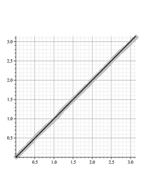
Figure 2: Left: Function $\arccos(2t-1)$ of real roots in $(0,1)$, against uniform distribution in $(0,\pi)$. Right: Density of polynomials in the Bernstein basis for $d\in\{5,10,15\}$.

As far as the distribution of the real roots in $(0,1)$ is concerned, if we denote them by $t_{i}$, then $\arccos(2t_{i}-1)$, behaves as the uniform distribution in $(0,\pi)$. In Fig. 2, we present the probability-probability plot, (using the ProbabilityPlot command of maple) of this function of real roots of random polynomials in Bernstein basis, of degree 1000 (light grey line), against the theoretical uniform distribution (black line) in $(0,\pi)$. We observe that the lines almost match. For reasons of space, we postpone the discussion about the distribution of the roots.

$d$	$\sqrt{2d}$	$(-\infty,\infty)$	$(-\infty,-1)$	$(-1,0)$	$(0,1)$	$(1,\infty)$
100	14.142	13.640	0.760	2.740	6.530	3.610
150	17.321	16.540	0.890	3.260	8.090	4.300
200	20.000	19.740	1.100	3.780	9.740	5.120
250	22.361	21.400	1.350	3.970	10.610	5.470
300	24.495	24.320	1.270	4.760	12.300	5.990
350	26.458	26.540	1.620	5.100	13.400	6.420
400	28.284	27.980	1.490	5.430	14.080	6.980
450	30.000	29.460	1.620	5.890	14.970	6.980
500	31.623	31.200	1.830	5.960	15.620	7.790
550	33.166	32.740	1.770	6.360	16.290	8.320
600	34.641	34.300	1.850	6.570	17.270	8.610
650	36.056	35.480	2.050	6.840	17.240	9.350
700	37.417	37.200	2.160	7.510	18.650	8.880
750	38.730	38.180	2.190	7.300	19.360	9.330
800	40.000	39.160	2.220	7.830	19.490	9.620
850	41.231	40.420	2.130	8.010	20.320	9.960
900	42.426	41.780	2.390	8.070	20.530	10.790
950	43.589	42.680	2.200	8.330	21.570	10.580
1000	44.721	43.540	2.400	8.610	21.770	10.760

Table 1: Experiments with random polynomial in the Bernstein basis.

5 Conclusions and future work

Our results explain why the solvers are fast in general, since typically there are few real roots and in general the separation bound is good enough. This agrees with the fact that in most cases the practical complexity of the sturm solver is dominated by the computation of the sequence and not by the evaluation. Our current work extends the first part of this paper to Kac polynomials, and to solvers descartes and bernstein.

The main issue with the Kac polynomials is that there is a discontinuity at $\pm 1$ when $d\rightarrow\infty$. To be more precise, the fact that there are few roots even near $\pm 1$, where they are concentrated asymptotically, is balanced by the fact the 2-point correlation, $k(s_{1},s_{2})$, between two consecutive roots is a complicated function of $|s_{1}-s_{2}|$, $s_{1}$ and $d$ and (in opposition with the two other distributions we studied) its limit when $d$ tends to infinity is not equivalent to a simple function of $|s_{1}-s_{2}|$. This is an interesting problem which deserves to be studied and investigate further.

An interesting question is whether we can design a randomized exact algorithm based on the properties of random polynomials. Lastly, we wish to extend our study to polynomials with inexact coefficients.

Acknowledgement. We thank the reviewers for their constructive comments. IZE thanks D. Hristopoulos for discussions on the statistics of roots’ distributions. AG acknowledge fruitful discussions with Julien Barre. IZE and AG are partially supported by Marie-Curie Network “SAGA”, FP7 contract PITN-GA-2008-214584. ET is partially supported by an individual postdoctoral grant from the Danish Agency for Science, Technology and Innovation, and by the State Scholarship Foundation of Greece.

References

- [1] A. Akritas. An implementation of Vincent’s theorem. Numerische Mathematik, 36:53–62, 1980.
- [2] D. Armentano and J.-P. Dedieu. A note about the average number of real roots of a Bernstein polynomial system. J. Complexity, 25(4):339 – 342, 2009.
- [3] A. T. Bharucha-Reid and M. Sambandham. Random Polynomials. Academic Press, 1986.
- [4] P. Bleher and X. Di. Correlations between zeros of a random polynomial. J. Stat. Physics, 88(1):269–305, 1997.
- [5] A. Bloch and G. Polya. On the roots of certain algebraic equations. Proc. London Math. Soc, 33:102–114, 1932.
- [6] C-P. Chen and F. Qi. The best bound in Wallis’ inequality. Proc. AMS, 133(2):397–401, 2004.
- [7] J. H. Davenport. Cylindrical algebraic decomposition. Technical Report 88–10, School of Mathematical Sciences, University of Bath, England, http://www.bath.ac.uk/masjhd/, 1988.
- [8] Z. Du, V. Sharma, and C. K. Yap. Amortized bound for root isolation via Sturm sequences. In D. Wang and L. Zhi, editors, Int. Workshop on Symbolic Numeric Computing, pages 113–129, Beijing, China, 2005. Birkhauser.
- [9] A. Edelman and E. Kostlan. How may zeros of a random polynomial are real? Bulletin AMS, 32(1):1–37, 1995.
- [10] A. Eigenwillig, V. Sharma, and C. K. Yap. Almost tight recursion tree bounds for the Descartes method. In Proc. Annual ACM ISSAC, pages 71–78, New York, USA, 2006.
- [11] I. Z. Emiris, B. Mourrain, and E. P. Tsigaridas. Real Algebraic Numbers: Complexity Analysis and Experimentation. In P. Hertling, C. Hoffmann, W. Luther, and N. Revol, editors, Reliable Implementations of Real Number Algorithms: Theory and Practice, volume 5045 of LNCS, pages 57–82, 2008.
- [12] P. Erdös and P. Turán. On the distribution of roots of polynomials. Annals of Mathematics, 51(1):105–119, 1950.
- [13] J.M. Hammersley. The zeros of a random polynomial. In Proc. of the 3rd Berkeley Symposium on Mathematical Statistics and Probability, volume 1955, pages 89–111, 1954.
- [14] J.H. Hannay. Chaotic analytic zero points: exact statistics for those of a random spin state. J. Physics A: Math. & General, 29:L101–L105, 1996.
- [15] L. E. Heindel. Integer arithmetic algorithms for polynomial real zero determination. J. of the Association for Computing Machinery, 18(4):533–548, October 1971.
- [16] H. Hong. Bounds for absolute positiveness of multivariate polynomials. J. Symbolic Comp., 25(5):571–585, 1998.
- [17] C. P. Hughes and A. Nikeghbali. The zeros of random polynomials cluster uniformly near the unit circle. Compositio Mathematica, 144:734–746, Mar 2008.
- [18] J. R. Johnson. Algorithms for Polynomial Real Root Isolation. PhD thesis, The Ohio State University, 1991.
- [19] J. R. Johnson, W. Krandick, K. Lynch, D. Richardson, and A. Ruslanov. High-performance implementations of the Descartes method. In Proc. Annual ACM ISSAC, pages 154–161, NY, 2006.
- [20] M. Kac. On the average number of real roots of a random algebraic equation. Bulletin AMS, 49:314–320 & 938, 1943.
- [21] E. Kowalski. Bernstein polynomials and Brownian motion. American Mathematical Monthly, 113(10):865–886, 2006.
- [22] W. Krandick. Isolierung reeller nullstellen von polynomen. In J. Herzberger, editor, Wissenschaftliches Rechnen, pages 105–154. Akademie-Verlag, Berlin, 1995.
- [23] T. Lickteig and M-F. Roy. Sylvester-Habicht Sequences and Fast Cauchy Index Computation. J. Symb. Comput., 31(3):315–341, 2001.
- [24] J.E. Littlewood and A.C. Offord. On the number of real roots of a random algebraic equation. J. London Math. Soc, 13:288–295, 1938.
- [25] K. Mehlhorn and S. Ray. Faster algorithms for computing Hong’s bound on absolute positiveness. J. Symbolic Computation, 45(6):677 – 683, 2010.
- [26] M. Mignotte and D. Ştefănescu. Polynomials: An algorithmic approach. Springer, 1999.
- [27] V.Y. Pan. Univariate polynomials: Nearly optimal algorithms for numerical factorization and rootfinding. J. Symbolic Computation, 33(5):701–733, 2002.
- [28] A. Papoulis and S.U. Pillai. Probability, random variables, and stochastic processes. McGraw-Hill, 3rd edition, 1991.
- [29] D. Reischert. Asymptotically fast computation of subresultants. In Proc. Annual ACM ISSAC, pages 233–240, 1997.
- [30] F. Rouillier and Z. Zimmermann. Efficient isolation of polynomial’s real roots. J. Comput. & Applied Math., 162(1):33–50, 2004.
- [31] G. Schehr and S.N. Majumdar. Real roots of random polynomials and zero crossing properties of diffusion equation. J. Stat. Physics, 132(2):235–273, 2008.
- [32] A. Schönhage. The fundamental theorem of algebra in terms of computational complexity. Manuscript. Univ. of Tübingen, Germany, 1982.
- [33] V. Sharma. Complexity of real root isolation using continued fractions. Theor. Comput. Sci., 409(2):292–310, 2008.
- [34] M. Shub and S. Smale. Complexity of bézout’s theorem II: volumes and probabilities. In F. Eyssette and A. Galligo, editors, Computational Algebraic Geometry, volume 109 of Progress in Mathematics, pages 267–285. Birkhäuser, 1993.
- [35] E. P. Tsigaridas and I. Z. Emiris. On the complexity of real root isolation using Continued Fractions. Theoretical Computer Science, 392:158–173, 2008.
- [36] C.K. Yap. Fundamental Problems of Algorithmic Algebra. Oxford University Press, New York, 2000.