Turing patterns in network-organized activator-inhibitor systems

Abstract

Turing instability in activator-inhibitor systems provides a paradigm of nonequilibrium pattern formation; it has been extensively investigated for biological and chemical processes. Turing pattern formation should furthermore be possible in network-organized systems, such as cellular networks in morphogenesis and ecological metapopulations with dispersal connections between habitats, but investigations have so far been restricted to regular lattices and small networks. Here we report the first systematic investigation of Turing patterns in large random networks, which reveals their striking difference from the known classical behavior. In such networks, Turing instability leads to spontaneous differentiation of the network nodes into activator-rich and activator-low groups, but ordered periodic structures never develop. Only a subset of nodes having close degrees (numbers of links) undergoes differentiation, with its characteristic degree obeying a simple general law. Strong nonlinear restructuring process leads to multiple coexisting states and hysteresis effects. The final stationary patterns can be well understood in the framework of the mean-field approximation for network dynamics.

I Introduction

In 1952, A. Turing published a seminal paper Turing , demonstrating that differences in diffusion rates of reacting species can alone destabilize the uniform state of the system and lead to the formation of spatial patterns and suggesting this as a possible mechanism of biological morphogenesis. The Turing instability and resulting patterns have subsequently been theoretically analyzed and experimentally confirmed for various chemical, biological, and ecological systems Prigogine ; Mimura ; DeKepper ; Ouyang ; Sick ; they are generally viewed as a paradigm of nonequilibrium pattern formation. In 1971, Othmer and Scriven Othmer pointed out that the Turing instability is also possible in network-organized systems and this should be important for the understanding of multi-cellular morphogenesis. At an early stage of the organism development, a network of inter-cellular connections is formed and morphogens are diffusively transported over such a network; differentiation of cells may thus be induced by the network Turing instability. On the other hand, many ecosystems represent metapopulations distributed over discrete habitats forming networks with dispersal connections Hanski ; Urban . Prey and predator or host and parasite species may migrate over such networks with different diffusional mobilities. Recently, diffusional spreading of infectious diseases over airline transportation networks has attracted much attention Hufnagel . Epidemic dynamics on the networks can be described by reaction-diffusion models where infected and susceptible individuals play the role of interacting species Murray ; Liu . In all such network-organized systems with diffusional transport of interacting species, the Turing instabilities and resulting nonlinear patterns can generally be expected.

Although nonlinear dynamics on complex networks is attracting significant attention, most of the investigations have focused on synchronization phenomena of oscillator networks (see, e.g., recent reviews Boccaletti ; Arenas ). Despite the potential importance of network Turing patterns and the large amount of research on classical Turing patterns in spatially extended systems, very little research on this problem has been performed so far. Early studies by Othmer and Scriven Othmer ; Othmer2 have provided abstract mathematical framework for the analysis of network Turing instability, but they explicitly considered only simple examples of regular lattices close in their properties to continuous media. Recently, Horsthemke et. al. Horsthemke ; Moore have discussed the possibility of Turing instability in coupled chemical reactors, but only for small networks.

In this article, we present the systematic analytical and numerical study of the Turing instability and of the developing nonlinear patterns in large random networks. We find that the Turing instability generally occurs in network-organized activator-inhibitor systems, but its properties are very different from those characteristic for the classical continuous media.

II Network-organized activator-inhibitor systems

Classical activator-inhibitor systems in continuous media are described by equations of the form

$$\frac{\partial}{\partial t}u({\bm{x}},t) = f(u,v)+D_{act}\nabla^{2}u({\bm{x}},t),$$ (1)

$$\frac{\partial}{\partial t}v({\bm{x}},t) = g(u,v)+D_{inh}\nabla^{2}v({\bm{x}},t),$$ (3)

where $u({\bm{x}},t)$ and $v({\bm{x}},t)$ are local densities of the activator and inhibitor species. Here, the functions $f(u,v)$ and $g(u,v)$ specify dynamics of the activator that autocatalytically enhances its own production and of the inhibitor that suppresses the activator growth. $D_{act}$ and $D_{inh}$ are the diffusion constants of the activator and inhibitor species. The classical Turing instability Turing sets in as the ratio $D_{inh}/D_{act}$ of the two diffusion constants is increased and exceeds a threshold. It leads to spontaneous development of alternating activator-rich and activator-low domains from the uniform background.

In our study, we consider the network analog of the model (3), where activator and inhibitor species occupy discrete nodes of a network and are diffusively transported over the links connecting them. We consider a connected network consisting of $N$ nodes, $i=1,\cdots,N$. The network topology is defined by a symmetric adjacency matrix whose elements $A_{ij}$ take values $A_{ij}=1$ if the nodes $i$ and $j$ are connected $(i\neq j)$ and $A_{ij}=0$ otherwise. Diffusive transport of the species into a certain node $i$ is simply given by the sum of incoming fluxes to the node $i$ from other connected nodes $\{j\}$, where the fluxes are proportional to the concentration difference between the nodes (Fick’s law). By introducing the network Laplacian matrix whose elements are given by $L_{ij}=A_{ij}-k_{i}\delta_{ij}$, where $k_{i}=\sum_{j=1}^{N}A_{ij}$ is the degree of the node $i$, diffusive flux of the species $u$ to node $i$ is expressed as $\sum_{j=1}^{N}L_{ij}u_{j}=\sum_{j=1}^{N}A_{ij}(u_{j}-u_{i})$, and similarly for $v$. Generally, diffusional mobilities of species $u$ and $v$ on the network are different. The equations describing network-organized activator-inhibitor systems are thus given by

$$\frac{d}{dt}u_{i}(t) = f(u_{i},v_{i})+\varepsilon\sum_{j=1}^{N}L_{ij}u_{j},$$ (4)

$$\frac{d}{dt}v_{i}(t) = g(u_{i},v_{i})+\sigma\varepsilon\sum_{j=1}^{N}L_{ij}v_{j},$$ (6)

for $i=1,\cdots,N$. Here, $f(u,v)$ and $g(u,v)$ specify the local activator-inhibitor dynamics on individual nodes. We denote the diffusional mobility of the activator species as $\varepsilon(=D_{act})$ and of the inhibitor species as $\sigma\varepsilon(=D_{inh})$, so that $\sigma=D_{inh}/D_{act}$ is the ratio between them. The considered systems have a uniform stationary state $(\bar{u},\bar{v})$, where $f(\bar{u},\bar{v})=0$ and $g(\bar{u},\bar{v})=0$. This uniform state can become unstable as a result of the Turing instability. If $u$ and $v$ correspond to the activator and inhibitor species, functions $f$ and $g$ should satisfy several conditions which are given in the Methods section.

As the examples of activator-inhibitor systems, we use the Mimura-Murray model of prey-predator populations Mimura and the classical Brusselator model Prigogine which are described in the Methods section. This study is focused on the Turing instability and pattern formation in large random networks. We use scale-free networks which are ubiquitous in Nature Barabasi ; Barabasi2 ; Boccaletti ; Arenas and the classical Erdös-Rényi random networks Barabasi ; Barabasi2 , both described in the Methods section. For convenience, network nodes $\{i\}$ are always sorted below in the decreasing order of their degrees $\{k_{i}\}$, so that the condition $k_{1}\geq k_{2}\geq\cdots k_{N}$ holds.

III The Turing instability

The Turing instability is revealed through the linear stability analysis of the uniform stationary state with respect to nonuniform perturbations (see Methods for the details). In the classical case of continuous media Turing , nonuniform perturbations are decomposed over a set of spatial Fourier modes, representing plane waves with different wavenumbers. As has been originally noticed by Othmer and Scriven Othmer , in the networks, the role of plane waves should be played by eigenvectors of their Laplacian matrices. The eigenvalues $\Lambda_{\alpha}$ and eigenvectors ${\bm{\phi}}^{(\alpha)}=(\phi_{1}^{(\alpha)},\cdots,\phi_{N}^{(\alpha)})$ of the Laplacian matrix $L_{ij}$ are determined Boccaletti ; Mohar by $\sum_{j=1}^{N}L_{ij}\phi_{j}^{(\alpha)}=\Lambda_{\alpha}\phi_{i}^{(\alpha)}$, with $\alpha=1,\cdots,N$. All eigenvalues of $L_{ij}$ are non-positive. We sort the indices $\{\alpha\}$ in the decreasing order of the eigenvalues, so that the condition $0=\Lambda_{1}\geq\Lambda_{2}\geq\cdots\geq\Lambda_{N}$ always holds.

Introducing small perturbations $(\delta u_{i},\delta v_{i})$ to the uniform state as $(u_{i},v_{i})=(\bar{u},\bar{v})+(\delta u_{i},\delta v_{i})$ and substituting this into equations (6), a set of coupled linearized differential equations is obtained. By expanding the perturbations over the set of Laplacian eigenvectors as $\delta u_{i}(t)=\sum_{\alpha=1}^{N}c_{\alpha}\exp\left[\lambda_{\alpha}t\right]\phi_{i}^{(\alpha)}$ and $\delta v_{i}(t)=\sum_{\alpha=1}^{N}c_{\alpha}B_{\alpha}\exp\left[\lambda_{\alpha}t\right]\phi_{i}^{(\alpha)}$, these equations are transformed into $N$ independent linear equations for different normal modes. The linear growth rate $\lambda_{\alpha}$ of the $\alpha$-th mode is determined from the characteristic equation. When $\mbox{Re}\ \lambda_{\alpha}$ is positive, the $\alpha$-th mode is unstable. The Turing instability takes place when one of the modes (i.e., the critical mode) begins to grow. At the instability threshold, $\mbox{Re }\lambda_{\alpha}=0$ for some $\alpha=\alpha_{c}$ and $\mbox{Re }\lambda_{\alpha}<0$ for all other modes. In the Turing instability, the critical mode is not oscillatory, $\mbox{Im}\ \lambda_{\alpha_{c}}$ = 0.

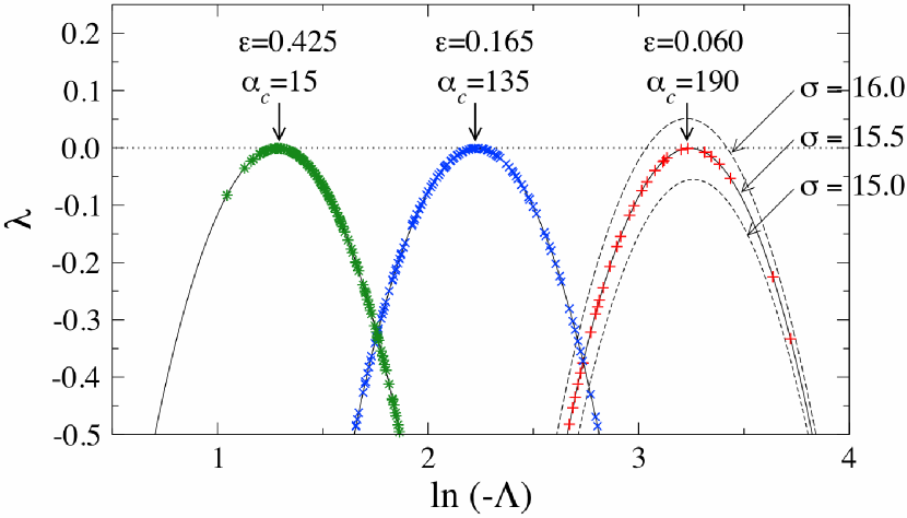
Figure 1: Linear stability analysis. Linear growth rates $\lambda_{\alpha}$ of the Laplacian modes $\alpha=1,\cdots,N$ for the Mimura-Murray model on a scale-free network ($N=200$ nodes and mean degree $\langle k\rangle=10$) for three values of the diffusional mobility $\varepsilon$ and for the critical ratio of diffusion constants $\sigma=15.5\simeq\sigma_{c}$. Three curves corresponding $\varepsilon=0.425$, $0.165$, and $0.060$ are plotted as functions of the Laplacian eigenvalues $\Lambda_{\alpha}$. For comparison, curves with $\sigma=15.0$ and $\sigma=16.0$ are also drawn for $\varepsilon=0.060$. Critical modes are indicated for each value of $\varepsilon$. The critical modes and the corresponding Laplacian eigenvalues are $\alpha_{c}=15$, $\Lambda_{c}=-3.62$ for $\varepsilon=0.425$, $\alpha_{c}=135$, $\Lambda_{c}=-9.32$ for $\varepsilon=0.165$, and $\alpha_{c}=190$, $\Lambda_{c}=-25.3$ for $\varepsilon=0.060$.

As an example, Fig. 1 shows the growth rate $\lambda$ as a function of $\Lambda$ for the Mimura-Murray model. At $\varepsilon=0.060$, three curves corresponding to different ratios $\sigma$ of diffusion constants (below, at and above the instability threshold) are displayed. In this figure, critical curves for two other values of the parameter $\varepsilon$ are also shown.

Generally, the Turing instability becomes possible for $\sigma>\sigma_{c}$. The dispersion curve $\lambda=F(\varepsilon\Lambda)$ first touches the horizontal axis at $\Lambda=\Lambda_{c}$ and the Laplacian mode $\phi_{i}^{(\alpha_{c})}$, possessing the Laplacian eigenvalue $\Lambda_{\alpha_{c}}$ that is closest to $\Lambda_{c}$, becomes critical. For the critical mode, the coefficient $B_{\alpha}$ is positive, so that when the activator concentration increases, the inhibitor concentration also increases accordingly. Explicit expressions are given in the Methods section. Note that the Laplacian spectrum of a network is discrete and, therefore, the instability actually occurs only when one of the respective points on the dispersion curve crosses the horizontal axis.

The above results are analogous to those holding for continuous media (cf. Mikhailov ). The critical ratio $\sigma_{c}$ in the networks is the same as in the classical case. The Laplacian eigenvalue $\Lambda_{c}$ of the critical network mode corresponds to $-q_{c}^{2}$, where $q_{c}$ is the wavenumber of the critical mode in the continuous media. Despite such formal analogies, properties of the network Turing patterns are very much different from their classical counterparts, as demonstrated in the following sections.

IV Localization of Laplacian eigenvectors and characteristic properties of critical Turing modes

When a Turing pattern starts to grow after slightly exceeding the instability threshold, the activator distribution in this pattern is determined by the critical Laplacian eigenvector, i.e. we have $\delta u_{i}\propto\phi_{i}^{(\alpha_{c})}$. Therefore, to understand organization of the growing Turing patterns, properties of Laplacian eigenvectors should be considered.

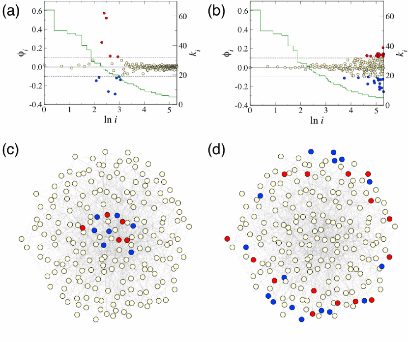
Figure 2: Critical Turing modes for a scale-free network of size $N=200$ and mean degree $\langle k\rangle=10$. (a,b): Critical eigenvectors (a) $\alpha_{c}=190$ and (b) $\alpha_{c}=15$ plotted against the node index $i$. Node degrees $k_{i}$ are shown by green stepwise curves. Node indices $\{i\}$ are sorted according to their degrees $\{k_{i}\}$. (c,d): The same critical eigenvectors (c) $\alpha_{c}=190$ and (d) $\alpha_{c}=15$ displayed graphically on the network.

As an example, Figs. 2(a,b) display critical eigenvectors of a network for two different values of the diffusion constant $\varepsilon$. The same eigenvectors are shown graphically in Figs. 2(c,d). In the chosen representation, network nodes with larger degrees (hubs) are located in the center and the nodes with lower degrees in the periphery of the graph. The nodes are colored red when $\phi_{i}^{(\alpha_{c})}\geq 0.1$ (e.g. activator concentration is significantly increased), blue when $\phi_{i}^{(\alpha_{c})}\leq-0.1$ (significantly decreased), and yellow for $-0.1<\phi_{i}^{(\alpha_{c})}<0.1$ (no significant change).

It is clearly seen in Fig. 2 that spontaneous differentiation of the nodes takes place - the distinguishing feature of the Turing instability. However, it affects only a fraction of all nodes. The differentiated nodes, with significant deviations of the activation level, tend to have close degrees. When the diffusional mobility $\varepsilon$ is small, only a subset of hub nodes undergoes differentiation [Figs. 2(a),(c)]. If $\varepsilon$ is large, differentiated nodes have just a few links [Figs. 2(b),(d)]. Thus, a correlation between the characteristic degrees of the differentiated nodes and the diffusional mobility is present. The behavior observed in Fig. 2 is general. As we show below, it is related to the effect of localization of Laplacian eigenvectors in large random networks.

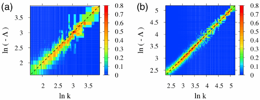
Figure 3: Localization of Laplacian eigenvectors in scale-free networks. The network size and mean degree are (a) $N=200$, $\langle k\rangle=10$ and (b) $N=1000$, $\langle k\rangle=20$. All nodes are divided into groups with equal degrees. For each group, the number of “differentiated” nodes with $\phi_{i}^{(\alpha)}\geq 0.1$ or $\phi_{i}^{(\alpha)}\leq-0.1$ for each eigenvector $\alpha$ is counted. Then the fraction of such nodes in each group for each Laplacian eigenvector $\alpha$ is determined. Thus, these diagrams show density distributions of differentiated nodes for the entire set of Laplacian eigenvectors.

As has recently been discussed Menzinger , Laplacian eigenvectors in large random networks with relatively broad degree distributions tend to localize on subsets of nodes with close degrees. The localization effect for a scale-free network is illustrated in Fig. 3. Here, all nodes are divided into groups with equal degrees $k$. For each group $k$ and a given Laplacian eigenvalue $\Lambda$, the number of “differentiated” nodes with $\phi_{i}^{(\alpha)}\geq 0.1$ or $\phi_{i}^{(\alpha)}\leq-0.1$ in the respective eigenvector $\phi_{i}^{(\alpha)}$ is counted. The density diagrams in Fig. 3 display in the color code the relative numbers of such nodes as functions of the Laplacian eigenvalue $\Lambda$ and the degree $k$. Examining Fig. 3, one can see that differentiated nodes are approximately located along the diagonal of the density map. The localization effect is more pronounced for the larger network of size $N=1000$. Similar localization behavior is observed for the Erdös-Rényi networks (see Supplementary information). Thus, we see that each Laplacian eigenvector $\phi_{i}^{(\alpha)}$ is characterized by its characteristic localization degree $\bar{k}_{\alpha}$. Moreover, this characteristic degree is approximately equal to the negative of the respective eigenvalue, so that a simple relationship $\bar{k}_{\alpha}\simeq-\Lambda_{\alpha}$ holds.

On the other hand, as implied by the linear stability analysis (see Methods), the growth rate $\lambda_{\alpha}$ of each mode depends only on the combination $\varepsilon\Lambda_{\alpha}$ of the diffusional mobility $\varepsilon$ and the eigenvalue $\Lambda_{\alpha}$ of that mode, i.e. we have $\lambda_{\alpha}=F(\varepsilon\Lambda_{\alpha})$. Therefore, the Laplacian eigenvalue $\Lambda_{\alpha_{c}}$ of the critical mode $\alpha_{c}$ with $\lambda_{\alpha_{c}}=0$ should be inversely proportional to the diffusive mobility $\varepsilon$, i.e., $\Lambda_{\alpha_{c}}\propto 1/\varepsilon$. Hence, modes with large negative eigenvalues $\Lambda_{\alpha}$ tend to become unstable for the small mobilities $\varepsilon$ (note that $\Lambda_{\alpha}\leq 0$ in our definition).

Combining the two relationships, $\bar{k}_{\alpha}\simeq-\Lambda_{\alpha}$ and $\Lambda_{\alpha_{c}}\propto 1/\varepsilon$, a simple scaling law $\bar{k}_{\alpha_{c}}\propto 1/\varepsilon$ is obtained. It implies that the characteristic degree $\bar{k}_{\alpha_{c}}$ of the differentiating subset is inversely proportional to the diffusional mobility $\varepsilon$.

The dependence $\Lambda_{\alpha_{c}}\propto 1/\varepsilon$ holds for any activator-inhibitor model exhibiting the Turing instability. The localization of Laplacian eigenvectors has been observed by us (to be separately published) also for other random networks with relatively broad degree distributions. The characteristic localization degree $\bar{k}_{\alpha_{c}}$ of the critical Turing mode is generally a monotonously increasing function of the negative of the critical Laplacian eigenvalue, $-\Lambda_{\alpha_{c}}$, and thus a decreasing function of the diffusional mobility $\varepsilon$.

V Stationary Turing patterns

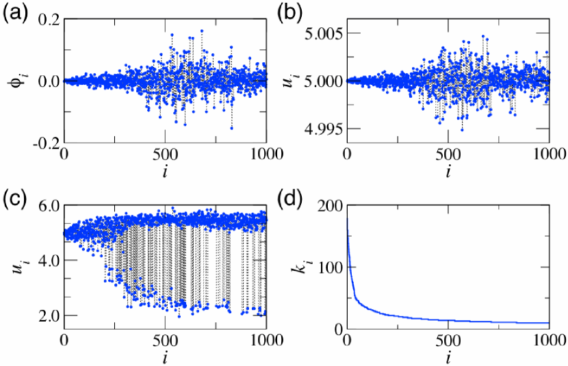
Figure 4: Nonlinear evolution and a stationary Turing pattern of the Mimura-Murray model on a scale-free network at $\epsilon=0.12$ and $\sigma=15.6$. The network size and mean degree are $N=1000$ and $\langle k\rangle=20$. (a) The critical mode (the Laplacian eigenvector with $\alpha_{c}=422$), (b) the activator pattern at the early evolution stage ($t=200$), and (c) the stationary activator pattern at the late stage ($t=1500$). Nodes are ordered according to their degrees; with (d) showing the dependence of the degree on the node index.

The initial exponential growth is followed by a nonlinear process, leading to the formation of stationary Turing patterns. The nonlinear evolution of the system and the properties of emerging stationary patterns have been studied by us in numerical simulations. Figure 4 presents typical results, obtained for intermediate diffusional mobility $(\varepsilon=0.12)$ and slightly above the instability threshold $(\sigma=15.6)$ for the Mimura-Murray model on the random scale-free network of size $N=1000$ and mean degree $\langle k\rangle=20$. The nodes are sorted in the order of their degrees, as shown in Fig. 4(d).

Starting from almost uniform initial conditions with small perturbations, exponential growth is observed at the early stage. The activator pattern at this stage, Fig. 4(b), is similar to the critical mode, Fig. 4(a), with the deviations due to the contributions from neighboring modes that are already excited to some extent. Later on, however, strong nonlinear effects develop, and the final stationary pattern, Fig. 4(c), becomes very different from the one determined by the critical mode.

Observing the nonlinear development, we notice that some nodes get progressively kicked off the main group near the destabilized uniform solution in this process (see Video in the Supplementary information). Eventually, in the asymptotic stationary state, the nodes become separated into two groups. The separation into two groups occurs only for the nodes with relatively small degrees (roughly $i>200$, $k_{i}<24$), while the nodes with high degrees ($i<200$, $k_{i}>24$) do not undergo the differentiation.

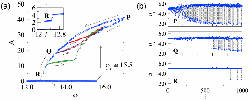
Figure 5: Hysteresis and multistability. (a) Amplitude $A$ of the Turing pattern vs. the diffusion ratio $\sigma$; variation directions of $\sigma$ are indicated by arrows. The inset shows the blowup near $R$. (b) Stationary Turing patterns at the parameter points $P$ ($\sigma=17.0$), $Q$ ($\sigma=13.5$), and $R$ ($\sigma=12.8$).

Our numerical investigations furthermore reveal that the outcome of nonlinear evolution depends sensitively on initial conditions. Different Turing patterns are possible at the same parameter values and strong hysteresis effects are observed. As an example, Fig. 5(a) shows how the amplitude of the stationary Turing pattern, defined as $A=\left[\sum_{i=1}^{N}\left\{(u_{i}-\bar{u})^{2}+(v_{i}-\bar{v})^{2}\right\}\right]^{1/2}$, varies under gradual variation of the parameter $\sigma$ in the upward or downward directions. Stationary patterns observed at points $P$, $Q$, and $R$ in Fig. 5(a) are shown in Fig. 5(b).

As $\sigma$ was increased starting from the uniform initial condition, the Turing instability took place at $\sigma=\sigma_{c}$, with the amplitude $A$ suddenly jumping up to a high value that corresponds to the appearance of a kicked-off group. If $\sigma$ was further increased, the amplitude $A$ grew. Starting to decrease $\sigma$, we did not however observe a drop down at $\sigma=\sigma_{c}$. Instead, a punctuated decrease in the amplitude $A$, which is characterized by many relatively small steps, was found. Reversing the direction of change of the parameter $\sigma$ at different points, many coexisting solution branches could be identified. The characteristics of Turing patterns vary with their amplitudes. When $A$ is close to zero [ point $R$ in Fig. 5(a) ], only a few kicked-off nodes remain in the system. Such localized Turing patterns with only a small number of destabilized nodes can coexist with the linearly stable uniform state and are found below the Turing instability threshold, for $\sigma<\sigma_{c}$.

VI The mean-field theory

To understand properties of the developed Turing patterns above the instability boundary ($\sigma>\sigma_{c}$), one can use the mean-field approximation, similar to that previously employed in the investigations of epidemics spreading on networks Pastor and for the networks of phase oscillators Ichinomiya . We start by writing equations (6) in the form

$$\frac{d}{dt}u_{i}(t) = f(u_{i},v_{i})+\varepsilon(h_{i}^{(u)}-k_{i}u_{i}),$$ (7)

$$\frac{d}{dt}v_{i}(t) = g(u_{i},v_{i})+\sigma\varepsilon(h_{i}^{(v)}-k_{i}v_{i}),$$ (9)

where local fields felt by each node, $h_{i}^{(u)}=\sum_{j=1}^{N}A_{ij}u_{j}$ and $h_{i}^{(v)}=\sum_{j=1}^{N}A_{ij}v_{j}$, are introduced. These local fields are further approximated as $h_{i}^{(u)}\simeq k_{i}H^{(u)}$ and $h_{i}^{(v)}\simeq k_{i}H^{(v)}$, where global mean fields are defined by $H^{(u)}=\sum_{j=1}^{N}w_{j}u_{j}$ and $H^{(v)}=\sum_{j=1}^{N}w_{j}v_{j}$. The weights $w_{j}=k_{j}/\left(\sum_{\ell=1}^{N}k_{\ell}\right)=k_{j}/k_{total}$ take into account the difference in contributions of different nodes to the global mean field, depending on their degrees (cf. Pastor ; Ichinomiya ). Thus, the local fields are taken to be proportional to the degree of a node, ignoring the details of its actual connections.

With this approximation, the individual activator-inhibitor system on each node interacts only with the global mean fields, and its dynamics is described by

$$\frac{d}{dt}u(t) = f(u,v)+\beta(H^{(u)}-u),$$ (10)

$$\frac{d}{dt}v(t) = g(u,v)+\sigma\beta(H^{(v)}-v).$$ (12)

We have dropped here the index $i$, since all nodes obey the same equations, and introduced the parameter $\beta(i)=\varepsilon k_{i}$. If diffusion ratio $\sigma$ is fixed and the global mean fields $H^{(u)}$ and $H^{(v)}$ are given, the parameter $\beta$ plays the role of a bifurcation parameter that controls the dynamics of each node. Equations (12) have a single stable fixed point when $\beta=0$ (i.e. $\varepsilon=0$), and, as $\beta$ is increased, this system typically undergoes a saddle-node bifurcation that gives rise to a new stable fixed point.

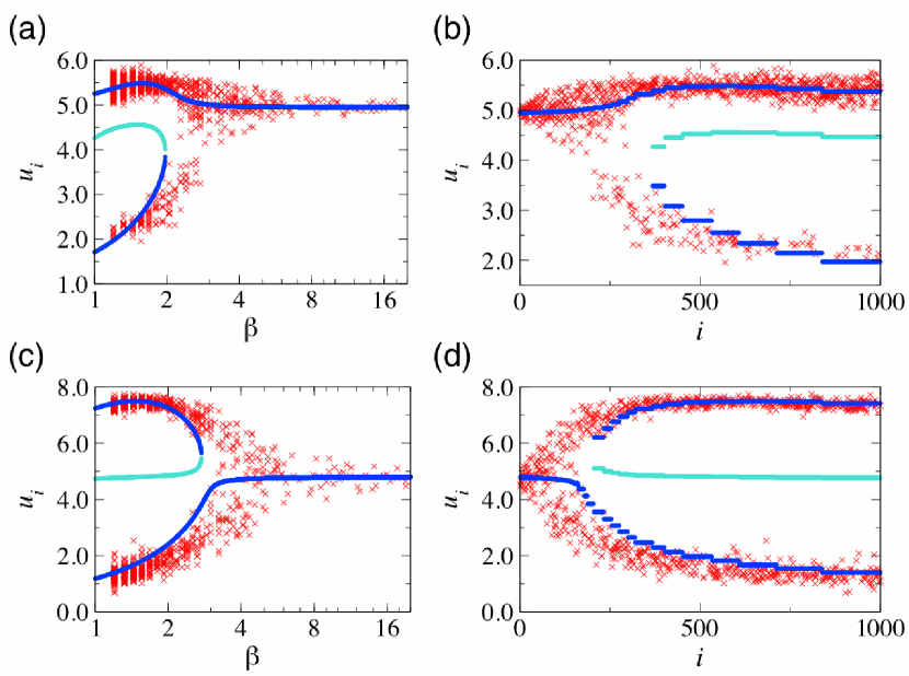
Figure 6: Developed Turing patterns and mean-field bifurcation diagrams. Stationary Turing patterns compared with the bifurcation diagrams of the activator-inhibitor system on a single node coupled to global mean fields. The parameters are $\varepsilon=0.12$ and (a,b) $\sigma=15.6$, (c,d) $\sigma=30$. Blue curves (dots) indicate stable branches and light-blue curves (dots) correspond to the unstable branches. Crosses show the computed Turing patterns. The global mean fields are $(H^{(u)},H^{(v)})=(4.95,9.97)$ for $\sigma=15.6$ and $(H^{(u)},H^{(v)})=(4.8,9.9)$ for $\sigma=30$.

As an example, we have computed stationary Turing patterns for the Mimura-Murray model by numerical integration of equations (6) and determined the respective global mean fields $H^{(u)}$ and $H^{(v)}$ at $\sigma=15.6$ and $\sigma=30$. Substituting these computed global mean fields into equations (12), bifurcation diagrams for a single node have been obtained (solid curves in Fig. 6 (a,c)). In this example, one of the two stable branches vanishes by another saddle-node bifurcation when $\beta$ is increased further. These diagrams can be compared with the actual stationary Turing patterns. Each node $i$ in the network is characterized by its degree $k_{i}$, so that it possesses a certain value of the bifurcation parameter, $\beta=\varepsilon k_{i}$. Therefore, the Turing pattern can be projected onto these bifurcation diagrams, as shown by crosses in Fig. 6(a,c). We see a relatively good agreement between the stable branches and the data from the actual Turing patterns. Furthermore, we directly compare in Fig. 6(b,d) the computed Turing patterns with the mean-field predictions, based on equations (12). The Turing patterns are well fitted by the stable branches, though the scattering of numerical data gets enhanced near the branching points.

In the Supplementary information, a similar analysis is performed for the Brusselator model. This model has a different bifurcation diagram in the presence of external fields. Nonetheless, a good agreement with the predictions of the mean-field theory is again observed. Thus, fully developed Turing patterns in the networks are essentially explained by the bifurcation diagrams of a single node coupled to global mean fields, with the coupling strength determined by the degree of the respective network node. The mean-field theory is generally not applicable for the localized Turing patterns found below the Turing instability threshold.

VII Discussion and conclusions

The fingerprint property of the classical Turing instability in continuous media is the spontaneous formation of periodic patterns above the critical point. Our investigations of the Turing problem for large random networks have revealed that, while the bifurcation remains essentially the same, properties of the emerging patterns are strongly different. In the networks, the critical Turing mode is localized on a subset of network nodes with the degrees close to a characteristic degree controlled by the mobility of species. The final stationary patterns are much different from the critical mode. Multistability, i.e. coexistence of a number of various stationary patterns for the same parameter values, is typically found and the hysteresis phenomena are observed. Above the instability threshold, network Turing patterns can be well understood in the framework of the mean-field approximation. In this approximation, each network element is coupled to certain global fields collectively determined by the entire system, and interactions of the element with its neighbor nodes are neglected. The strength of coupling to the global fields depends on the number of links connecting an element to the rest of the network.

The Turing instability is also possible in regular lattices representing a special case of networks. An activator-inhibitor system on a lattice can be viewed as a finite-difference approximation for the respective reaction-diffusion problem in the space and Turing patterns on the lattices should therefore have almost the same properties as in the continuous media. The divergent behavior, characteristic for large random networks, must be related to a difference in the structural properties of such systems. Diameters of random networks are relatively small and nodes in such networks cannot be separated by large distances (roughly estimated as $L=\ln N$ for the Erdös-Rényi and scale-free networks Havlin ). For comparison, a cubic lattice with $N$ nodes in the $d$-dimensional space has the diameter about $L=N^{1/d}$. Thus, a lattice with the same size $N$ as a random network and a comparable diameter $L$ must have a high dimension $d\gg 1$. In lattices with high dimensionality and short lengths, Turing patterns with many alternating domains are however not possible and just a few domains (clusters) shall be found, resembling what is indeed observed by us in large random networks.

Because of their small diameters, diffusional mixing in random networks is strong. Large random networks are, therefore, structurally much closer to the globally coupled systems than to the low-dimensional lattices. Globally coupled activator-inhibitor populations have previously been considered and spontaneous separation of the elements into two groups has also been found in such systems Mizuguchi . There is, however, an important further aspect distinguishing random networks from the lattices or simple globally coupled systems. All nodes in a lattice (or in a globally coupled population) are equivalent and have the same degree (number of neighbors). In contrast to this, random networks effectively represent strongly heterogeneous systems. They are characterized by broad degree distributions (less broad but still relatively wide for the finite-size Erdös-Rényi networks). This heterogeneity becomes essential in the problems involving diffusion. Under the same concentration gradients across the links, a node with a higher degree receives a larger incoming flux from the neighboring nodes.

The heterogeneity is responsible for the localization of Laplacian eigenvectors on the subsets of nodes with close degrees. Laplacian eigenvectors of networks are known to play an important role in the synchronization phenomena. However, only the second and the last of such eigenvectors are significant there (see  Boccaletti ). In contrast, in network Turing problems, the entire Laplacian spectrum becomes significant. By varying the diffusional mobility of species, critical Turing modes corresponding to different Laplacian eigenvectors are realized.

In the present study, a general framework for the analysis of network Turing patterns has been proposed. Numerical investigations, confirming the theory, have been performed for the ecological predator-prey Mimura-Murray model Mimura and for the classical chemical Brusselator model Prigogine . Both models belong to the activator-inhibitor class. There is moreover a different broad class of models where the first species is characterized by autocatalytic growth (i.e., represents an activator) and it consumes for its growth the second species which effectively represents a renewable resource (see, e.g., Mikhailov ). In these systems, growth of the activator leads to the depletion of the renewable resource, which has an inhibitory effect on the activator. The considered Turing instabilities should also exist in such other network-organized systems.

The results of our study may be important in a broad range of applications. Turing instabilities can generally be expected in various cellular, ecological or epidemic networks in Nature and their detection and observation represent a major scientific challenge. With the progress in engineering of synthetic ecosystems Weber , artificial ecological networks exhibiting Turing patterns can be designed in the future.

VIII Methods

Since $u$ is the activator and $v$ is the inhibitor in equations (6), partial derivatives of $f(u,v)$ and $g(u,v)$ at $(\bar{u},\bar{v})$ should satisfy the following conditions: $f_{u}=\left.\partial f/\partial u\right|_{(\bar{u},\bar{v})}>0$, $f_{v}=\left.\partial f/\partial u\right|_{(\bar{u},\bar{v})}<0$, $g_{u}=\left.\partial g/\partial u\right|_{(\bar{u},\bar{v})}>0$, and $g_{v}=\left.\partial g/\partial v\right|_{(\bar{u},\bar{v})}<0$. The uniform stationary state of the system $(u_{i},v_{i})=(\bar{u},\bar{v})$ for all $i=1,\cdots,N$ is assumed to be linearly stable in the absence of diffusion, which requires $f_{u}+g_{v}<0$ and $f_{u}g_{v}-f_{v}g_{u}>0$.

In the Mimura-Murray model Mimura , $u$ and $v$ correspond to the prey and the predator densities. In this model, we have $f(u,v)=\{(a+bu-u^{2})/c-v\}u$ and $g(u,v)=\{u-(1+dv)\}v$, where the parameters have been chosen as $a=35$, $b=16$, $c=9$, and $d=2/5$ in the present study, yielding the fixed point $(\bar{u},\bar{v})=(5,10)$. In the Brusselator model Prigogine , variables $u$ and $v$ correspond to densities of chemical activator and inhibitor species. Here we have $f(u,v)=p-(r+1)u+u^{2}v$ and $g(u,v)=ru-u^{2}v$ and the parameters have been chosen as $p=1$ and $r=1.8$. The fixed point is $(\bar{u},\bar{v})=(1,1.8)$.

Scale-free networks are generated by the preferential attachment algorithm of Barábasi and Albert Barabasi ; Barabasi2 , in which nodes with larger degrees tend to acquire more links. Starting from $m$ fully connected initial nodes, we are adding $m$ new connections at each iteration step, so that the mean degree is $\langle k\rangle\simeq 2m$. The simple Erdös-Rényi networks are generated by preparing $N$ nodes and then randomly connecting two arbitrary nodes with probability $q$, yielding the mean degree of $\langle k\rangle\simeq Nq$ Barabasi2 .

The Laplacian $L_{ij}$ of any network is a real, symmetric, and negative semi-definite matrix Mohar . All eigenvalues are real and non-positive. The eigenvectors are orthonormalized as $\sum_{i=1}^{N}\phi_{i}^{(\alpha)}\phi_{i}^{(\beta)}=\delta_{\alpha,\beta}$ where $\alpha,\beta=1,\cdots,N$.

The linear stability analysis is performed in close analogy to the classical case of continuous media. Small perturbations $\delta u_{i}$ and $\delta v_{i}$ obey linearized differential equations

$$\frac{d}{dt}{\delta u}_{i}(t) = f_{u}\delta u_{i}+f_{v}\delta v_{i}+\varepsilon\sum_{j=1}^{N}L_{ij}\delta u_{j},$$ (13)

$$\frac{d}{dt}{\delta v}_{i}(t) = g_{u}\delta u_{i}+g_{v}\delta v_{i}+\sigma\varepsilon\sum_{j=1}^{N}L_{ij}\delta v_{j}.$$ (15)

Expanding $\delta u_{i}$ and $\delta v_{i}$ over the Laplacian normal modes $\phi_{i}^{(\alpha)}$ as described in the main text, the following eigenvalue equation is obtained:

$$\lambda_{\alpha}\left(\begin{array}[]{c}1\cr B_{\alpha}\end{array}\right)=\left(\begin{array}[]{cc}f_{u}+\varepsilon\Lambda_{\alpha}&f_{v}\cr g_{u}&g_{v}+\sigma\varepsilon\Lambda_{\alpha}\end{array}\right)\left(\begin{array}[]{c}1\cr B_{\alpha}\end{array}\right).$$ (16)

From the characteristic equation $\{\lambda_{\alpha}-f_{u}-\varepsilon\Lambda_{\alpha}\}\{\lambda_{\alpha}-g_{v}-\sigma\varepsilon\Lambda_{\alpha}\}-f_{v}g_{u}=0$, a pair of conjugate growth rates are obtained for each Laplacian mode as $\lambda_{\alpha}=(1/2)\{f_{u}+g_{v}+(1+\sigma)\varepsilon\Lambda_{\alpha}\pm[4f_{v}g_{u}+\left(f_{u}-g_{v}+(1-\sigma)\varepsilon\Lambda_{\alpha}\right)^{2}]^{1/2}\}$. Only the upper branch can become positive and it is always chosen as $\lambda_{\alpha}$ in our analysis. From the condition that $\lambda_{\alpha}$ touches the horizontal axis at its maximum, the critical value of $\sigma$ is determined as $\sigma_{c}=\{f_{u}g_{v}-2f_{v}g_{u}+2[f_{v}g_{u}(f_{v}g_{u}-f_{u}g_{v})]^{1/2}\}/f_{u}^{2}$ and the critical Laplacian eigenvalue is determined for a given $\varepsilon$ as $\Lambda_{c}=\{(f_{u}-g_{v})\sigma_{c}-\sqrt{|f_{v}|g_{u}\sigma_{c}}(\sigma_{c}+1)\}/\{\varepsilon\sigma_{c}(\sigma_{c}-1)\}$. The critical eigenvector in the $(u,v)$ plane is given by $(1,B_{c})$ where $B_{c}=\{-f_{u}+g_{v}+(\sigma_{c}-1)\varepsilon\Lambda_{c}+[4f_{v}g_{u}+\left(f_{u}-g_{v}-(\sigma_{c}-1)(\varepsilon\Lambda_{c})\right)^{2}]^{1/2}\}/(2f_{v})$. These expressions coincide with the respective expressions for the continuous media (see, e.g., Mikhailov ), if we replace there $\Lambda$ by $-q^{2}$, where $q$ is the wavenumber of the plane wave mode.

Acknowledgments

Financial support of the Volkswagen Foundation (Germany) and the MEXT (Japan, Kakenhi 19762053) is gratefully acknowledged.

Competing financial interests

The authors declare no competing financial interests.

References

- (1) Turing, A. M., The chemical basis of morphogenesis, Phil. Trans. R. Soc. London B: Biol. Sci. 237, 37 (1952).
- (2) Prigogine, I. and Lefever, R. Symmetry breaking instabilities in dissipative systems. II. J. Chem. Phys. 48, 1695 (1968).
- (3) Mimura, M. and Murray, J. D., Diffusive prey-predator model which exhibits patchiness, J. Theor. Biol. 75, 249 (1978).
- (4) Castets, V., Dulos, E., Boissonade, J. and De Kepper, P., Experimental evidence of a sustained standing Turing-type nonequilibrium chemical pattern, Phys. Rev. Lett. 64, 2953 (1990).
- (5) Ouyang, Q. and Swinney, H. L., Transition from a uniform state to hexagonal and striped Turing patterns, Nature 352, 610 (1991).
- (6) Sick, S., et al., WNT and DKK determine hair follicle spacing through a reaction-diffusion mechanism, Science 314, 1447 (2006).
- (7) Othmer, H. G., Scriven, L. E., Instability and dynamic pattern in cellular networks, J. Theor. Biol. 32, 507 (1971).
- (8) Hanski, I., Metapopulation dynamics, Nature 396, 41 (1998).
- (9) Urban, D., and Keitt, T., Landscape connectivity: a graph-theoretic perspective, Ecology 82, 1205 (2001).
- (10) Hufnagel, L., Brockmann, D., and Geisel, T., Forecast and control of epidemics in a globalized world, Proc. Natl. Acad. Sci. USA 101, 15124 (2004).
- (11) Murray, J. D., Mathematical Biology, Springer, Belin, 2003.
- (12) Liu, Q. -X., and Jin, Z., Formation of spatial patterns in epidemic model with constant removal rate of the infectives, J. Stat. Mech. P05002 (2007).
- (13) Boccaletti, S., Latora, V., Moreno, Y., Chavez, M., and Hwang, D.-U., Complex networks: structure and dynamics, Phys. Rep. 424, 175 (2006).
- (14) Arenas, A., Díaz-Guilera, A., Kurths, J., Moreno, Y., and Zhou, C., Synchronization in complex networks, Phys. Rep. 469, 93 (2008).
- (15) Othmer, H. G., Scriven, L. E., Nonlinear aspects of dynamic pattern in cellular networks, J. Theor. Biol. 43, 83 (1974).
- (16) Horsthemke, W., Lam, K., and Moore, P. K., Network topology and Turing instability in small arrays of diffusively coupled reactors, Phys. Lett. A 328, 444 (2004).
- (17) Moore, P. K., and Horsthemke, W., Localized patterns in homogeneous networks of diffusively coupled reactors, Physica D 206, 121 (2005).
- (18) Barabási, A.-L., and Albert, R., Emergence of scaling in random networks, Science 286, 509 (1999).
- (19) Albert, R., and Barabási, A.-L., Statistical mechanics of complex networks, Rev. Mod. Phys. 74, 47 (2002).
- (20) Mohar, B., The Laplacian spectrum of graphs, in Graph Theory, Combinatorics and Applications, Y. Alavi et al., Eds., New York: Wiley, 1991, pp. 871-898.
- (21) Mikhailov A. S., Foundations of Synergetics I. Distributed Active Systems (2nd revised edition), Springer, 1994.
- (22) McGraw, P. N., and Menzinger, M., Laplacian spectra as a diagnostic tool for network structure and dynamics, Phys. Rev. E 77 031102 (2008).
- (23) Pastor-Satorras R., and Vespignani, A., Epidemic spreading in scale-free networks, Phys. Rev. Lett. 86 3200 (2001).
- (24) Ichinomiya, T., Frequency synchronization in a random oscillator network, Phys. Rev. E 70 026116 (2004).
- (25) Cohen, R. and Havlin, S., Scale-free networks are ultrasmall, Phys. Rev. Lett. 90, 058701 (2003).
- (26) Mizuguchi, T., and Sano, M., Proportion regulation of biological cells in globally coupled nonlinear systems, Phys. Rev. Lett. 75, 966 (1995).
- (27) Weber, W., Baba, M. D.-E. and Fussenegger, M., Synthetic ecosystems based on airborne inter- and intrakingdom communication, Proc. Natl. Acad. Sci. USA 104, 10435 (2007).