The solution path of the generalized lasso

Abstract

We present a path algorithm for the generalized lasso problem. This problem penalizes the $\ell_{1}$ norm of a matrix $D$ times the coefficient vector, and has a wide range of applications, dictated by the choice of $D$. Our algorithm is based on solving the dual of the generalized lasso, which greatly facilitates computation of the path. For $D=I$ (the usual lasso), we draw a connection between our approach and the well-known LARS algorithm. For an arbitrary $D$, we derive an unbiased estimate of the degrees of freedom of the generalized lasso fit. This estimate turns out to be quite intuitive in many applications.

keywordAMSAMS 2010 subject classification.

and

1 Introduction.

Regularization with the $\ell_{1}$ norm seems to be ubiquitous throughout many fields of mathematics and engineering. In statistics, the best-known example is the lasso, the application of an $\ell_{1}$ penalty to linear regression lasso , bp . Let $y\in\mathbb{R}^{n}$ be a response vector and $X\in\mathbb{R}^{n\times p}$ be a matrix of predictors. If the response and the predictors have been centered, we can omit an intercept term from the model, and then the lasso problem is commonly written as

$$\operatorname{minimize}\limits_{\beta\in\mathbb{R}^{p}}\frac{1}{2}\|y-X\beta\|_{2}^{2}+\lambda\|\beta\|_{1},$$ (1)

where $\lambda\geq 0$ is a tuning parameter. There are many fast algorithms for solving the lasso (1) at a single value of the parameter $\lambda$, or over a discrete set of parameter values. The least angle regression (LARS) algorithm, on the other hand, is unique in that it solves (1) for all $\lambda\in[0,\infty]$ lars (see also the earlier homotopy method of homotopy , and the even earlier work of parqp ). This is possible because the lasso solution is piecewise linear with respect to $\lambda$.

The LARS path algorithm may provide a computational advantage when the solution is desired at many values of the tuning parameter. For large problems, this is less likely to be the case because the number of knots (changes in slope) in the solution path tends to be very large, and this renders the path intractable. Computational efficiency aside, the LARS method fully characterizes the tradeoff between goodness-of-fit and sparsity in the lasso solution (this is controlled by $\lambda$), and hence yields interesting statistical insights into the problem. Most notably, the LARS paper established a result on the degrees of freedom of the lasso fit, which was further developed by lassodf .

The first of its kind, LARS inspired the development of path algorithms for various other optimization problems that appear in statistics svmpath , rosset , holger , dasso , and our case is no exception. In this paper, we derive a path algorithm for problems that use the $\ell_{1}$ norm to enforce certain structural constraints—instead of pure sparsity—on the coefficients in a linear regression. These problems are nicely encapsulated by the formulation:

$$\operatorname{minimize}\limits_{\beta\in\mathbb{R}^{p}}\frac{1}{2}\|y-X\beta\|_{2}^{2}+\lambda\|D\beta\|_{1},$$ (2)

where $D\in\mathbb{R}^{m\times p}$ is a specified penalty matrix. We refer to problem (2) as the generalized lasso. Depending on the application, we choose $D$ so that sparsity of $D\beta$ corresponds to some other desired behavior for $\beta$, typically one that is structural or geometric in nature. In fact, various choices of $D$ in (2) give problems that are already well-known in the literature: the fused lasso, trend filtering, wavelet smoothing, and a method for outlier detection. We derive a simple path algorithm for the minimization (2) that applies to a general matrix $D$, hence this entire class of problems. Like the lasso, the generalized lasso solution is piecewise linear as a function of $\lambda$. We also prove a result on the degrees of freedom of the fit for a general $D$. It is worth noting that problem (2) has been considered by other authors, for example, tisp . This last work establishes some asymptotic properties of the solution, and proposes a computational technique that relates to simulated annealing.

The paper is organized as follows. We begin in Section 2 by motivating the use of a penalty matrix $D$, offering several examples of problems that fit into this framework. Section 3 explains that some instances of the generalized lasso can be transformed into a regular lasso problem, but many cannot, emphasizing the need for a new path approach. In Section 4, we derive the Lagrange dual of (2), which serves as the jumping point for our algorithm and all of the work that follows. For the sake of clarity, we build up the algorithm over the next 3 sections. Sections 5 and 6 consider the case $X=I$. In Section 5, we assume that $D$ is the 1-dimensional fused lasso matrix, in which case our path algorithm takes an especially simple (and intuitive) form. In Section 6, we give the path algorithm for a general penalty matrix $D$, which requires adding only one step in the iterative loop. Section 7 extends the algorithm to the case of a general design matrix $X$. Provided that $X$ has full column rank, we show that our path algorithm still applies, by rewriting the dual problem in a more familiar form. We also outline a path approach for the case when $X$ has rank less than its number of columns. Practical considerations for the path’s computation are given in Section 8.

In Section 9, we focus on the lasso case, $D=I$, and compare our method to LARS. Above, we described LARS as an algorithm for computing the solution path of (1). This actually refers to LARS in its “lasso” state, and although this is probably the best-known version of LARS, it is not the only one. In its original (unmodified) state, LARS does not necessarily optimize the lasso criterion, but instead performs a more “democratic” form of forward variable selection. It turns out that with an easy modification, our algorithm gives this selection procedure exactly. In Section 10, we derive an unbiased estimate of the degrees of freedom of the fit for a general matrix $D$. The proof is quite straightforward because it utilizes the dual fit, which is simply the projection onto a convex set. As we vary $D$, this result yields interpretable estimates of the degrees of freedom of the fused lasso, trend filtering, and more. Finally, Section 11 contains some discussion.

To save space (and improve readability), many of the technical details in the paper are deferred to a supplementary document supp .

2 Applications.

There are a wide variety of interesting applications of problem (2). What we present below is not meant to be an exhaustive list, but rather a set of illustrative examples that motivated our work on this problem in the first place. This section is split into two main parts: the case when $X=I$ (often called the “signal approximation” case), and the case when $X$ is a general design matrix.

2.1 The signal approximation case, $X=I$.

When $X=I$, the solution of the lasso problem (1) is given by soft-thresholding the coordinates of $y$. Therefore, one might think that an equally simple formula exists for the generalized lasso solution when the design matrix is the identity—but this is not true. Taking $X=I$ in the generalized lasso (2) gives an interesting and highly nontrival class of problems. In this setup, we observe data $y\in\mathbb{R}^{n}$ which is a noisy realization of an underlying signal, and the rows of $D\in\mathbb{R}^{m\times n}$ reflect some believed structure or geometry in the signal. The solution of problem (2) fits adaptively to the data while exhibiting some of these structural properties. We begin by looking at piecewise constant signals, and then address more complex features.

2.1.1 The fused lasso.

Suppose that $y$ follows a 1-dimensional structure, that is, the coordinates of $y$ correspond to successive positions on a straight line. If $D$ is the $(n-1)\times n$ matrix

$$D_{\mathrm{1d}}=\left[\matrix{-1&1&0&\cdots&0&0\cr 0&-1&1&\cdots&0&0\cr&&&\cdots&&\cr 0&0&0&\cdots&-1&1}\right],$$ (3)

then problem (2) penalizes the absolute differences in adjacent coordinates of $\beta$, and is known as the 1d fused lasso fuse . This gives a piecewise constant fit, and is used in settings where coordinates in the true model are closely related to their neighbors. A common application area is comparative genomic hybridization (CGH) data: here $y$ measures the number of copies of each gene ordered linearly along the genome (actually $y$ is the log ratio of the number of copies relative to a normal sample), and we believe for biological reasons that nearby genes will exhibit a similar copy number. Identifying abnormalities in copy number has become a valuable means of understanding the development of many human cancers. See Figure 1 for an example of the 1d fused lasso applied to some CGH data on glioblastoma multiformes, a particular type of malignant brain tumor, taken from gbm .

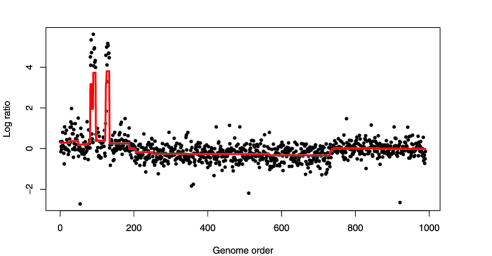
Figure 1: The 1d fused lasso applied to some glioblastoma multiforme data. The red line represents the inferred copy number from the 1d fused lasso solution (for $\lambda=3$).

A natural extension of this idea penalizes the differences between neighboring pixels in an image. Suppose that $y$ represents a noisy image that has been unraveled into a vector, and each row of $D$ again has a $1$ and $-1$, but this time arranged to give both the horizontal and vertical differences between pixels. Then problem (2) is called the 2d fused lasso fuse , and is used to denoise images that we believe should obey a piecewise constant structure. This technique is actually a special type of total variation denoising, a well-studied problem that carries a vast literature spanning the fields of statistics, computer science, electrical engineering, and others (see tv , e.g.). Figure 2 shows the 2d fused lasso applied to a toy example.

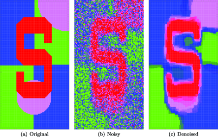
Figure 2: An example of the 2d fused lasso for image denoising. We started with a toy signal, shown in (a). The colors green, blue, purple, red in the image correspond to the numeric levels $1,2,3,4$, respectively. We then added noise, shown in (b), interpolating between colors to display the intermediate values. This is used as the data $y$ in the 2d fused lasso problem. The solution (for $\lambda=1$) is shown in (c), and it is a fairly accurate reconstruction. The method is effective here because the original image is piecewise constant.

We can further extend this idea by defining adjacency according to an arbitrary graph structure, with $n$ nodes and $m$ edges. Now the coordinates of $y\in\mathbb{R}^{n}$ correspond to nodes in the graph, and we penalize the difference between each pair of nodes joined by an edge. Hence $D$ is $m\times n$, with each row having a $-1$ and $1$ in the appropriate spots, corresponding to an edge in the graph. In this case, we simply call problem (2) the fused lasso. Note that both the 1d and 2d fused lasso problems are special cases of this, with the underlying graph a chain and a 2d grid, respectively. But the fused lasso is a very general problem, as it can be applied to any graph structure that exhibits a piecewise constant signal across adjacent nodes. See Figure 3 for application in which the underlying graph has US states as nodes, with two states joined by an edge if they share a border. This graph has 48 nodes (we only include the mainland US states) and 105 edges.

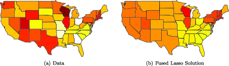
Figure 3: An example of the fused lasso on an irregular graph. The data $y$ are the log proportion of H1N1 flu cases for each (mainland) US state in the year 2009, shown in (a). This was taken from h1n1 . The color map uses white to reflect the lowest measured log proportion, and dark red to reflect the highest, with yellow, orange, and red in between. We can think of the data as noisy measurements of the true log probabilities of infection in each state, which likely exhibits some geographic trend. Therefore, we solve the fused lasso problem on a custom underlying graph, where we connect two states by an edge if they share a border. Shown in (b) is the solution (for $\lambda=0.25$). Here, groups of states are assigned the same color or “fused” on the west coast, in the mid west, in the south east, and in the north east. The colors suggest that, among these regions, you are most likely to get H1N1 flu if you live in the north east, then the west coast, then the midwest, and then the south east. But there certainly are states that do not get fused into these regions, like Wisconsin and Illinois, where the infection rates are exceptionally high.

The observant reader may notice a discrepancy between the usual fused lasso definition and ours, as the fused lasso penalty typically includes an additional term $\|\beta\|_{1}$, the $\ell_{1}$ norm of the coefficients themselves. We refer to this as the sparse fused lasso, and to represent this penalty we just append the $n\times n$ identity matrix to the rows of $D$. Actually, this carries over to all of the applications yet to be discussed—if we desire pure sparsity in addition to the structural behavior that is being encouraged by $D$, we append the identity matrix to the rows of $D$.

2.1.2 Linear and polynomial trend filtering.

Suppose again that $y$ follows a 1-dimensional structure, but now $D$ is the $(n-2)\times n$ matrix

$$D_{\mathrm{tf},1}=\left[\matrix{\displaystyle-1&2&-1&\cdots&0&0&0\cr\displaystyle 0&-1&2&\cdots&0&0&0\cr\displaystyle\cdots&&&&&&\cr\displaystyle 0&0&0&\cdots&-1&2&-1}\right].$$

Then problem (2) is equivalent to linear trend filtering (also called $\ell_{1}$ trend filtering) l1tf . Just as the 1d fused lasso penalizes the discrete first derivative, this technique penalizes the discrete second derivative, and so it gives a piecewise linear fit. This has many applications, namely, any settings in which the underlying trend is believed to be linear with (unknown) changepoints. Moreover, by recursively defining

$$D_{\mathrm{tf},k}=D_{\mathrm{1d}}\cdot D_{\mathrm{tf},k-1}\qquad\mbox{for }k=2,3,\ldots$$

[here $D_{\mathrm{1d}}$ is the $(n-k-1)\times(n-k)$ version of (3)], we can fit a piecewise polynomial of any order $k$, further extending the realm of applications. We call this polynomial trend filtering of order $k$. Figure 4 shows examples of linear, quadratic, and cubic fits.

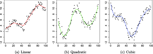
Figure 4: Solutions of (2) for three problems, with $D$ equal to (a) $D_{\mathrm{tf},1}$, (b) $D_{\mathrm{tf},2}$ and (c) $D_{\mathrm{tf},3}$. These are piecewise linear, quadratic and cubic, respectively. (For each problem we chose a different value of the regularization parameter $\lambda$.)

The polynomial trend filtering fits (especially for $k=3$) are similar to those that one could obtain using regression splines and smoothing splines. However, the knots (changes in $k$th derivative) in the trend filtering fits are selected adaptively based on the data, jointly with the inter-knot polynomial estimation. This phenomenon of simultaneous selection and estimation—analogous to that concerning the nonzero coefficients in the lasso fit, and the jumps in the piecewise constant fused lasso fit—does not occur in regression and smoothing splines. Regression splines operate on a fixed set of knots, and there is a substantial literature on knot placement for this problem (see Chapter 9.3 of gam , e.g.). Smoothing splines place a knot at each data point, and implement smoothness via a generalized ridge regression on the coefficients in a natural spline basis. As a result (of this $\ell_{2}$ shrinkage), they cannot represent both global smoothness and local wiggliness in a signal. On the other hand, trend filtering has the potential to represent both such features, a property called “time and frequency localization” in the signal processing field, though this idea has been largely unexplored. The classic example of a procedure that allows time and frequency localization is wavelet smoothing, discussed next.

2.1.3 Wavelet smoothing.

This is a quite a popular method in signal processing and compression. The main idea is to model the data as a sparse linear combination of wavelet functions. Perhaps the most common formulation for wavelet smoothing is SURE shrinkage sure , which solves the lasso optimization problem

$$\operatorname{minimize}\limits_{\theta\in\mathbb{R}^{n}}\frac{1}{2}\|y-W\theta\|_{2}^{2}+\lambda\|\theta\|_{1},$$ (4)

where $W\in\mathbb{R}^{n\times n}$ has an orthogonal wavelet basis along its columns. By orthogonality, we can change variables to $\beta=W\theta$ and then (4) becomes a generalized lasso problem with $D=W^{T}$.

In many applications it is desirable to use an overcomplete wavelet set, so that $W\in\mathbb{R}^{n\times m}$ with $n<m$. Now problem (4) and the generalized lasso (2) with $D=W^{T}$ (and $X=I$) are no longer equivalent, and in fact give quite different answers. In signal processing, the former is called the synthesis approach, and the latter the analysis approach, to wavelet smoothing. Though attention has traditionally been centered around synthesis, a recent paper by Elad, Milanfar and Rubinstein avs suggests that synthesis may be too sensitive, and shows that it can be outperformed by its analysis counterpart.

2.2 A general design matrix $X$.

For any of the fused lasso, trend filtering, or wavelet smoothing penalties discussed above, the addition of a general matrix $X$ of covariates significantly extends the domain of applications. For a fused lasso example, suppose that each row of $X$ represents a $k_{1}\times k_{2}\times k_{3}$ MRI image of a patient’s brain, unraveled into a vector (so that $p=k_{1}\cdot k_{3}\cdot k_{3}$). Suppose that $y$ contains some continuous outcome on the patients, and we model these as a linear function of the MRIs, $\mathrm{E}(y_{i}|X_{i})=\beta^{T}X_{i}$. Now $\beta$ also has the structure of a $k_{1}\times k_{2}\times k_{3}$ image, and by choosing the matrix $D$ to give the sparse 3d fused lasso penalty (i.e., the fused lasso on a 3d grid with an additional $\ell_{1}$ penalty of the coefficients), the solution of (2) attempts to explain the outcome with a small number of contiguous regions in the brain.

As another example, the inclusion of a design matrix $X$ in the trend filtering setup provides an alternative way of fitting varying-coefficient models vcm , lrm . We consider a data set from vcm , which examines $n=88$ observations on the exhaust from an engine fueled by ethanol. The response $y$ is the concentration of nitrogen dioxide, and the two predictors are a measure of the fuel-air ratio $E$, and the compression ratio of the engine $C$. Studying the interactions between $E$ and $C$ leads the authors of vcm to consider the model

$$\mathrm{E}(y_{i}|E_{i},C_{i})=\beta_{0}(E_{i})+\beta_{1}(E_{i})\cdot C_{i}.$$ (5)

This is a linear model with a different intercept and slope for each $E_{i}$, subject to the (implicit) constraint that the intercept and slope should vary smoothly along the $E_{i}$’s. We can fit this using (2), in the following way: first we discretize the continuous observations $E_{1},\ldots,E_{n}$ so that they lie into, say, 25 bins. Our design matrix $X$ is $88\times 50$, with the first 25 columns modeling the intercept $\beta_{0}$ and the last 25 modeling the slope $\beta_{1}$. The $i$th row of $X$ is

$$X_{ij}=\cases{\displaystyle 1,&\quad if $E_{i}$ lies in the $j$th bin,\cr\displaystyle C_{i},&\quad if $E_{i}$ lies in the $(j+25)$th bin,\cr\displaystyle 0,&\quad otherwise.}$$

Finally, we choose

$$D=\left[\matrix{\displaystyle D_{\mathrm{tf},3}&0\cr\displaystyle 0&D_{\mathrm{tf},3}}\right],$$

where $D_{\mathrm{tf},3}$ is the cubic trend filtering matrix (the choice $D_{\mathrm{tf},3}$ is not crucial and of course can be replaced by a higher or lower order trend filtering matrix). The matrix $D$ is structured in this way so that we penalize the smoothness of the first 25 and last 25 components of $\beta=(\beta_{0},\beta_{1})^{T}$ individually. With $X$ and $D$ as described, solving the optimization problem (2) gives the coefficients shown in Figure 5, which appear quite similar to the fits in vcm .

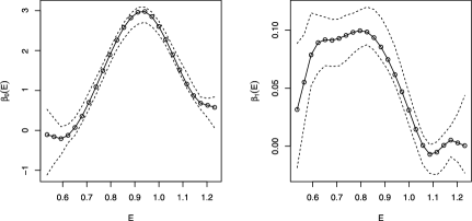
Figure 5: The intercept and slope of the varying-coefficient model (5) for the engine data of vcm , fit using (2) with a cubic trend filtering penalty matrix (and $\lambda=3$). The dashed lines show 85% bootstrap confidence intervals from 500 bootstrap samples.

We conclude this section with a generalized lasso application of owenoutlie , in which the penalty is not structurally-based, unlike the examples discussed previously. Suppose that we observe $y_{1},\ldots,y_{n}$, and we believe the majority of these points follow a linear model $\mathrm{E}(y_{i}|X_{i})=\beta^{T}X_{i}$ for some covariates $X_{i}=(X_{i1},\ldots,X_{ip})^{T}$, except that a small number of the $y_{i}$ are outliers and do not come from this model. To determine which points are outliers, one might consider the problem

$$\operatorname{minimize}\limits_{z\in\mathbb{R}^{n},\beta\in\mathbb{R}^{p}}\frac{1}{2}\|z-X\beta\|_{2}^{2}\qquad\mbox{subject to }\|z-y\|_{0}\leq k$$ (6)

for a fixed integer $k$. Here $\|x\|_{0}=\sum_{i}1(x_{i}\not=0)$. Thus by setting $k=3$, for example, the solution $\hat{z}$ of (6) would indicate which 3 points should be considered outliers, in that $\hat{z}_{i}\not=y_{i}$ for exactly 3 coordinates. A natural convex relaxation of problem (6) is

$$\operatorname{minimize}\limits_{z\in\mathbb{R}^{n},\beta\in\mathbb{R}^{p}}\frac{1}{2}\|z-X\beta\|_{2}^{2}+\lambda\|z-y\|_{1},$$ (7)

where we have also transformed the problem from bound form to Lagrange form. Letting $\alpha=y-z$, this can be rewritten as

$$\operatorname{minimize}\limits_{\alpha\in\mathbb{R}^{n},\beta\in\mathbb{R}^{p}}\frac{1}{2}\|y-\alpha-X\beta\|_{2}^{2}+\lambda\|\alpha\|_{1},$$ (8)

which fits into the form of problem (2), with design matrix $\widetilde{X}=\left[I\enskip X\right]$, coefficient vector $\tilde{\beta}=(\alpha,\beta)^{T}$, and penalty matrix $D=\left[I\enskip 0\right]$. Figure 6 shows a simple example with $p=1$.

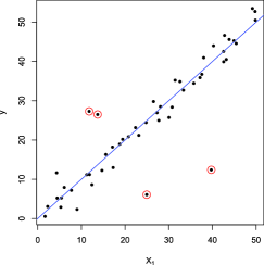
Figure 6: A simple example of using problem (2) to perform outlier detection. Written in the form (8), the blue line denotes the fitted slope $\hat{\beta}$, while the red circles indicate the outliers, as determined by the coordinates of $\hat{\alpha}$ that are nonzero (for $\lambda=8$).

After reading the examples in this section, a natural question is: when can a generalized lasso problem (2) be transformed into a regular lasso problem (1)? (Recall, e.g., that this is possible for an orthogonal $D$, as we discussed in the wavelet smoothing example.) We discuss this in the next section.

3 When does a generalized lasso problem reduce to a lasso problem?

If $D$ is $p\times p$ and invertible, we can transform variables in problem (2) by $\theta=D\beta$, yielding the lasso problem

$$\operatorname{minimize}\limits_{\theta\in\mathbb{R}^{p}}\frac{1}{2}\|y-XD^{-1}\theta\|^{2}_{2}+\lambda\|\theta\|_{1}.$$ (9)

More generally, if $D$ is $m\times p$ and $\operatorname{rank}(D)=m$ (note that this necessarily means $m\leq p$), then we can still transform variables and get a lasso problem. First, we construct a $p\times p$ matrix $\widetilde{D}=\left[{D\atop A}\right]$ with $\operatorname{rank}(\widetilde{D})=p$, by finding a $(p-m)\times p$ matrix $A$ whose rows are orthogonal to those in $D$. Then we change variables to $\theta=(\theta_{1},\theta_{2})^{T}=\widetilde{D}\beta$, so that the generalized lasso (2) becomes

$$\operatorname{minimize}\limits_{\theta\in\mathbb{R}^{p}}\frac{1}{2}\|y-X\widetilde{D}^{-1}\theta\|^{2}_{2}+\lambda\|\theta_{1}\|_{1}.$$ (10)

This is almost a regular lasso, except that the $\ell_{1}$ penalty only covers part of the coefficient vector. First, write $X\widetilde{D}^{-1}\theta=X_{1}\theta_{1}+X_{2}\theta_{2}$; then, it is clear that at the solution the second block of the coefficients is given by a linear regression:

$$\hat{\theta}_{2}=(X_{2}^{T}X_{2})^{-1}X_{2}^{T}(y-X_{1}\hat{\theta}_{1}).$$

Therefore, we can rewrite problem (10) as

$$\operatorname{minimize}\limits_{\theta_{1}\in\mathbb{R}^{m}}\frac{1}{2}\|(I-P)y-(I-P)X_{1}\theta_{1}\|^{2}_{2}+\lambda\|\theta_{1}\|_{1},$$ (11)

where $P=X_{2}^{T}(X_{2}^{T}X_{2})^{-1}X_{2}^{T}$, the projection onto the column space of $X_{2}$. The LARS algorithm provides the solution path of such a lasso problem (11), from which we can back-transform to get the generalized lasso solution: $\hat{\beta}=\widetilde{D}^{-1}\hat{\theta}$.

However, if $D$ is $m\times p$ and $\operatorname{rank}(D)<m$, then such a transformation is not possible, and LARS cannot be used to find the solution path of the generalized lasso problem (2). Further, in this case, the authors of avs establish what they call an “unbridgeable” gap between problems (1) and (2), based on the geometric properties of their solutions.

Table 1: Examples from Section 2 that fall into the cases $\operatorname{rank}(D)=m$ and $\operatorname{rank}(D)<m$

$\bolds{\operatorname{rank}(D)=m}$	$\bolds{\operatorname{rank}(D)<m}$
$\bullet$ The 1d fused lasso $\bullet$ Polynomial trend filtering of any order $\bullet$ Wavelet smoothing with an orthogonal $\bullet$ wavelet basis$\bullet$ Outlier detection	$\bullet$ The fused lasso on any graph that has $\bullet$ more edges $m$ than nodes $p$ (e.g., the 2d $\bullet$ fused lasso)$\bullet$ The sparse fused lasso on any graph $\bullet$ Wavelet smoothing with an overcomplete$\bullet$ wavelet set

While several of the examples from Section 2 satisfy $\operatorname{rank}(D)=m$, and hence admit a lasso transformation, a good number also fall into the case $\operatorname{rank}(D)<m$, and suggest the need for a novel path algorithm. These are summarized in Table 3. Therefore, in the next section, we derive the Lagrange dual of problem (2), which leads to a nice algorithm to compute the solution path of (2) for an arbitrary penalty matrix $D$.

4 The Lagrange dual problem.

First, we consider the generalized lasso in the signal approximation case, $X=I$:

$$\operatorname{minimize}\limits_{\beta\in\mathbb{R}^{n}}\frac{1}{2}\|y-\beta\|_{2}^{2}+\lambda\|D\beta\|_{1}.$$ (12)

Essentially, problem (12) is difficult to analyze directly because the nondifferentiable $\ell_{1}$ penalty is composed with a linear transformation of $\beta$. Following an argument of l1tf , we rewrite the problem as

$$\operatorname{minimize}\limits_{\beta\in\mathbb{R}^{n},z\in\mathbb{R}^{m}}\frac{1}{2}\|y-\beta\|_{2}^{2}+\lambda\|z\|_{1}\qquad\mbox{subject to }D\beta=z.$$

The Lagrangian is hence

$$\tfrac{1}{2}\|y-\beta\|_{2}^{2}+\lambda\|z\|_{1}+u^{T}(D\beta-z),$$

and to derive the dual problem, we minimize this over $\beta,z$. The terms involving $\beta$ are just a quadratic, and up to some constants (not depending on $u$)

$$\min_{\beta}\biggl{(}\frac{1}{2}\|y-\beta\|_{2}^{2}+u^{T}D\beta\biggr{)}=-\frac{1}{2}\|y-D^{T}u\|_{2}^{2},$$

while

$$\min_{z}(\lambda\|z\|_{1}-u^{T}z)=\cases{\displaystyle 0,&\quad if $\|u\|_{\infty}\leq\lambda$,\cr\displaystyle-\infty,&\quad otherwise.}$$

Therefore, the dual problem of (12) is

$$\operatorname{minimize}\limits_{u\in\mathbb{R}^{m}}\frac{1}{2}\|y-D^{T}u\|_{2}^{2}\qquad\mbox{subject to }\|u\|_{\infty}\leq\lambda.$$ (13)

Immediately, we can see that (13) has a “nice” constraint set, $\{u\dvtx\|u\|_{\infty}\leq\lambda\}$, which is simply a box, free of any linear transformation. It is also important to note the difference in dimension: the dual problem has a variable $u\in\mathbb{R}^{m}$, whereas the original problem (12), called the primal problem, has a variable $\beta\in\mathbb{R}^{n}$.

When $\operatorname{rank}(D)<m$, the dual problem is not strictly convex, and so it can have many solutions. On the other hand, the primal problem is always strictly convex and always has a unique solution. The primal problem is also strictly feasible (it has no constraints), and so strong duality holds (see Section 5.2 of convex ). The primal and dual solutions—written as $\hat{\beta}_{\lambda}$ and $\hat{u}_{\lambda}$, respectively, to emphasize the dependence on $\lambda$—are related by

$$\hat{\beta}_{\lambda}=y-D^{T}\hat{u}_{\lambda}.$$ (14)

Furthermore, each coordinate $i=1,\ldots,m$ of the dual solution satisfies

$$\hat{u}_{\lambda,i}\in\cases{\displaystyle\{+\lambda\},&\quad if $(D\hat{\beta}_{\lambda})_{i}>0$,\cr\displaystyle\{-\lambda\},&\quad if $(D\hat{\beta}_{\lambda})_{i}<0$,\cr\displaystyle[-\lambda,\lambda],&\quad if $(D\hat{\beta}_{\lambda})_{i}=0$.}$$ (15)

This last equation tells us that the dual coordinates that are equal to $\lambda$ in absolute value,

$$\mathcal{B}=\{i\dvtx|\hat{u}_{\lambda,i}|=\lambda\},$$ (16)

are the coordinates of $D\hat{\beta}_{\lambda}$ that are “allowed” to be nonzero. But this does necessarily mean that $(D\hat{\beta}_{\lambda})_{i}\not=0$ for all $i\in\mathcal{B}$.

For a general design matrix $X$, we can apply a similar argument to derive the dual of (2):

$$\operatorname{minimize}\limits_{u\in\mathbb{R}^{m}}\frac{1}{2}(X^{T}y-D^{T}u)^{T}(X^{T}X)^{+}(X^{T}y-D^{T}u)$$

(17)

$$\eqntext{\mbox{subject to }\|u\|_{\infty}\leq\lambda,\ D^{T}u\in\operatorname{row}(X).}$$ (18)

This looks complicated, certainly in comparison to problem (13). However, the inequality constraint on $u$ is still a simple (untransformed) box. Moreover, we can make (4) look like (13) by a change of variables. This will be discussed later in Section 7.

In the next two sections, Sections 5 and 6, we restrict our attention to the case $X=I$ and derive an algorithm to find a solution path of the dual (13). This gives the desired primal solution path, using the relationship (14). Since our focus is on solving the dual problem, we write simply “solution” or “solution path” to refer to the dual versions. Though we will eventually consider an arbitrary matrix $D$ in Section 6, we begin by studying the 1d fused lasso in Section 5. This case is especially simple, and we use it to build the framework for the path algorithm in the general case.

5 The 1d fused lasso.

In this setting, we have $D=D_{\mathrm{1d}}$, the $(n-1)\times n$ matrix given in (3). Now the dual problem (13) is strictly convex (since $D_{\mathrm{1d}}$ has rank equal to its number of rows), and therefore it has a unique solution. In order to efficiently compute the solution path, we use a lemma that allows us, at different stages, to reduce the dimension of the problem by one.

5.1 The boundary lemma.

Consider the constraint set $\{u\dvtx\|u\|_{\infty}\leq\lambda\}\subseteq\mathbb{R}^{n-1}$: this is a box centered around the origin with side length $2\lambda$. We say that coordinate $i$ of $u$ is “on the boundary” (of this box) if $|u_{i}|=\lambda$. For the 1d fused lasso, it turns out that coordinates of the solution that are on the boundary will remain on the boundary indefinitely as $\lambda$ decreases. This idea can be stated more precisely as follows.

Lemma 1 ((The boundary lemma)).

Suppose that $D=D_{\mathrm{1d}}$, the 1d fused lasso matrix in (3). For any coordinate $i$, the solution $\hat{u}_{\lambda}$ of (13) satisfies

$$\hat{u}_{\lambda_{0},i}=\lambda_{0}\quad\Rightarrow\quad\hat{u}_{\lambda,i}=\lambda\qquad\mbox{for all }\lambda\in[0,\lambda_{0}]$$

and

$$\hat{u}_{\lambda_{0},i}=-\lambda_{0}\quad\Rightarrow\quad\hat{u}_{\lambda,i}=-\lambda\qquad\mbox{for all }\lambda\in[0,\lambda_{0}].$$

The proof is given in supp . It is interesting to note a connection between the boundary lemma and a lemma of pco , which states that

$$\hat{\beta}_{\lambda_{0},i}=\hat{\beta}_{\lambda_{0},i+1}\quad\Rightarrow\quad\hat{\beta}_{\lambda,i}=\hat{\beta}_{\lambda,i+1}\qquad\mbox{for all }\lambda\geq\lambda_{0}$$ (19)

for this same problem. In other words, this lemma says that no two equal primal coordinates can become unequal with increasing $\lambda$. In general $|\hat{u}_{\lambda,i}|=\lambda$ is not equivalent to $(D\hat{\beta}_{\lambda})_{i}\not=0$, but these two statements are equivalent for the 1d fused lasso problem (see the primal-dual correspondence in Section 5.3), and therefore the boundary lemma is equivalent to (19).

5.2 Path algorithm.

This section is intended to explain the path algorithm from a conceptual point of view, and no rigorous arguments for its correctness are made here. We defer these until Section 6.1, when we revisit the problem in the context of a general matrix $D$.

The boundary lemma describes the behavior of the solution as $\lambda$ decreases, and therefore it is natural to construct the solution path by moving the parameter from $\lambda=\infty$ to $\lambda=0$. As will be made apparent from the details of the algorithm, the solution path is a piecewise linear function of $\lambda$, with a change in slope occurring whenever one of its coordinate paths hits the boundary. The key observation is that, by the boundary lemma, if a coordinate hits the boundary it will stay on the boundary for the rest of the path down to $\lambda=0$. Hence, when it hits the boundary we can essentially eliminate a coordinate from consideration (since we know its value at each smaller $\lambda$), recompute the slopes of the other coordinate paths, and move until another coordinate hits the boundary.

As we construct the path, we maintain two lists: $\mathcal{B}=\mathcal{B}(\lambda)$, which contains the coordinates that are currently on the boundary; and $s=s(\lambda)$, which contains their signs. For example, if we have $\mathcal{B}(\lambda)=(5,2)$ and $s(\lambda)=(-1,1)$, then this means that $\hat{u}_{\lambda,5}=-\lambda$ and $\hat{u}_{\lambda,2}=\lambda$. We call the coordinates in $\mathcal{B}$ the “boundary coordinates,” and the rest the “interior coordinates.” Now we can describe the algorithm:

Algorithm 1 ((Dual path algorithm for the 1d fused lasso)).

• Start with $\lambda_{0}=\infty$, $\mathcal{B}=\varnothing$ and $s=\varnothing$.

• For $k=0,\ldots,n-2$:

  1. [3.]

  2. Compute the solution at $\lambda_{k}$ by least squares, as in (21).

  3. Continuing in a linear direction from the solution, compute $\lambda_{k+1}$, when an interior coordinate will next hit the boundary, as in (22) and (23).

  4. Add this coordinate to $\mathcal{B}$ and its sign to $s$.

The algorithm’s details appear slightly more complicated, but this is only because of notation. If $\mathcal{B}=(i_{1},\ldots,i_{k})$, then we define for a matrix $A$ and a vector $x$

$$A_{\mathcal{B}}=\left[\matrix{A_{i_{1}}\cr\vdots\cr A_{i_{k}}}\right]\quad\mbox{and}\quad x_{\mathcal{B}}=(x_{i_{1}},\ldots,x_{i_{k}})^{T},$$

where $A_{i}$ is the $i$th row of $A$. In words: $A_{\mathcal{B}}$ indexes the rows of $A$ that are in $\mathcal{B}$, and $x_{\mathcal{B}}$ indexes the coordinates of $x$ in $\mathcal{B}$. We use the subscript $-\mathcal{B}$, as in $A_{-\mathcal{B}}$ or $x_{-\mathcal{B}}$, to index over all rows or coordinates except those in $\mathcal{B}$. Note that $\mathcal{B}$ as defined above (in the paragraph preceding the algorithm) is consistent with our previous definition (16), except that here we treat $\mathcal{B}$ as an ordered list instead of a set (its ordering only needs to be consistent with that of $s$). Also, we treat $s$ as a vector when convenient.

When $\lambda=\infty$, the problem is unconstrained, and so clearly $\mathcal{B}=\varnothing$ and $s=\varnothing$. But more generally, suppose that we are at the $k$th iteration, with boundary set $\mathcal{B}=\mathcal{B}(\lambda_{k})$ and signs $s=s(\lambda_{k})$. By the boundary lemma, the solution satisfies

$$\hat{u}_{\lambda,\mathcal{B}}=\lambda s\qquad\mbox{for all }\lambda\in[0,\lambda_{k}].$$

Therefore, for $\lambda\leq\lambda_{k}$, we can reduce the optimization problem (13) to

$$\operatorname{minimize}\limits_{u_{-\mathcal{B}}}\frac{1}{2}\|y-\lambda(D_{\mathcal{B}})^{T}s-(D_{-\mathcal{B}})^{T}u_{-\mathcal{B}}\|_{2}^{2}\qquad\mbox{subject to }\|u_{-\mathcal{B}}\|_{\infty}\leq\lambda,$$ (20)

which involves solving for just the interior coordinates. By construction, $\hat{u}_{\lambda_{k},-\mathcal{B}}$ lies strictly between $-\lambda_{k}$ and $\lambda_{k}$ in every coordinate. Therefore, it is found by simply minimizing the objective function in (20), which gives the least squares estimate

$$\hat{u}_{\lambda_{k},-\mathcal{B}}=(D_{-\mathcal{B}}(D_{-\mathcal{B}})^{T})^{-1}D_{-\mathcal{B}}\bigl{(}y-\lambda_{k}(D_{\mathcal{B}})^{T}s\bigr{)}.$$ (21)

Let $a-\lambda_{k}b$ denote the right-hand side above. For $\lambda\leq\lambda_{k}$, the interior solution will continue to be $\hat{u}_{\lambda,-\mathcal{B}}=a-\lambda b$ until one of its coordinates hits the boundary. This critical value is determined by solving, for each $i$, the equation $a_{i}-\lambda b_{i}=\pm\lambda$; a simple calculation shows that the solution is

$$t_{i}=\frac{a_{i}}{b_{i}\pm 1}=\frac{[(D_{-\mathcal{B}}(D_{-\mathcal{B}})^{T})^{-1}D_{-\mathcal{B}}y]_{i}}{[(D_{-\mathcal{B}}(D_{-\mathcal{B}})^{T})^{-1}D_{-\mathcal{B}}(D_{\mathcal{B}})^{T}s]_{i}\pm 1}$$ (22)

(only one of $+1$ or $-1$ will yield a value $t_{i}\in[0,\lambda_{k}]$), which we call the “hitting time” of coordinate $i$. We take $\lambda_{k+1}$ to be maximum of these hitting times

$$\lambda_{k+1}=\max_{i}t_{i}.$$ (23)

Then we compute

$$i_{k+1}=\operatorname{\arg\max}\limits_{i}t_{i}\quad\mbox{and}\quad s_{k+1}=\operatorname{sign}(\hat{u}_{\lambda_{k+1},i_{k+1}}),$$

and append $i_{k+1}$ and $s_{k+1}$ to $\mathcal{B}$ and $s$, respectively.

5.3 Properties of the solution path.

Here, we study some of the path’s basic properties. Again we defer any rigorous arguments until Section 6.2, when we consider a general penalty matrix $D$. Instead, we demonstrate them by way of a simple example.

Consider Figure 7(a), which shows the coordinate paths $\hat{u}_{\lambda,i}$ for an example with $n=8$. Recall that it is natural to interpret the paths from right to left ($\lambda=\infty$ to $\lambda=0$). Initially all of the slopes are zero, because when $\lambda=\infty$ the solution is just the least squares estimate $(DD^{T})^{-1}Dy$, which has no dependence on $\lambda$. When a coordinate path first hits the boundary (the topmost path, drawn in red) the slopes of the other paths change, and they do not change again until another coordinate hits the boundary (the bottommost path, drawn in green), and so on, until all coordinates are on the boundary.

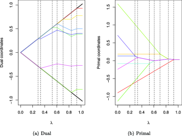
Figure 7: (a) Dual and (b) primal coordinate paths for a small problem with $n=8$.

The picture suggests that the path $\hat{u}_{\lambda}$ is continuous and piecewise linear with respect to $\lambda$, with changes in slope or “kinks” at the values $\lambda_{1},\ldots,\lambda_{n-1}$ visited by the algorithm. (Piecewise linearity is obvious from the algorithm’s construction of the path, but continuity is not.) This is also true in the general $D$ case, although the solution path can have more than $m$ kinks for an $m\times n$ matrix $D$.

On the other hand, Figure 7(b) shows the corresponding primal coordinate paths

$$\hat{\beta}_{\lambda,i}=(y-D^{T}\hat{u}_{\lambda})_{i}.$$

As $\hat{u}_{\lambda}$ is a continuous piecewise linear function of $\lambda$, so is $\hat{\beta}_{\lambda}$, again with kinks at $\lambda_{1},\ldots,\lambda_{n-1}$. In contrast to the dual versions, it is natural to interpret the primal coordinate paths from left to right, because in this direction the coordinate paths become adjoined, or “fused,” at a some value of $\lambda$. The primal picture suggests that these fusion values are the same as the kinks $\lambda_{1},\ldots,\lambda_{n-1}$, that is:

• Primal-dual correspondence for the 1d fused lasso. The values of $\lambda$ at which two primal coordinates fuse are exactly the values of $\lambda$ at which a dual coordinate hits the boundary.

A similar property holds for the fused lasso on an arbitrary graph, although the primal-dual correspondence is a little more complicated for this case.

Note that as $\lambda$ decreases in Figure 7(a), no dual coordinate paths leave the boundary. This is prescribed by the boundary lemma. As $\lambda$ increases in Figure 7(b), no primal two coordinates split apart, or “unfuse.” This is prescribed by a lemma of pco that we paraphrased in (19), and the two lemmas are equivalent.

6 A general penalty matrix $D$.

Now we consider (13) for general $m\times n$ matrix $D$. The first question that comes to mind is: does the boundary lemma still hold? If $DD^{T}$ is diagonally dominant, that is

$$(DD^{T})_{ii}\geq\sum_{j\not=i}|(DD^{T})_{ij}|\qquad\mbox{for }i=1,\ldots,m,$$ (24)

then indeed the boundary lemma is still true. (See supp .) Therefore, the path algorithm for such a $D$ is the same as that presented in the previous section.

It is easy to check the 1d fused lasso matrix is diagonally dominant, as both the left- and right-hand sides of the inequality in (24) are equal to 2 when $D=D_{\mathrm{1d}}$. Unfortunately, neither the 2d fused lasso matrix nor any of the trend filtering matrices satisfy condition (24). In fact, examples show that the boundary lemma does not hold for these cases. However, inspired by the 1d fused lasso, we can develop a similar strategy to compute the full solution path for an arbitrary matrix $D$. The difference is: in addition to checking when coordinates will hit the boundary, we have to check when coordinates will leave the boundary as well.

6.1 Path algorithm.

Recall that we defined, at a particular $\lambda_{k}$, the “hitting time” of an interior coordinate path to the value of $\lambda\leq\lambda_{k}$ at which this path hits the boundary. Similarly, let us define the “leaving time” of a boundary coordinate path to be the value of $\lambda\leq\lambda_{k}$ at which this path leaves the boundary (we will make this idea more precise shortly). We call the coordinate with the largest hitting time the “hitting coordinate,” and the one with the largest leaving time the “leaving coordinate.” As before, we maintain a list $\mathcal{B}$ of boundary coordinates, and $s$ contains their signs. The algorithm for a general matrix $D$ is:

Algorithm 2 ((Dual path algorithm for a general $D$)).

• Start with $k=0$, $\lambda_{0}=\infty$, $\mathcal{B}=\varnothing$, and $s=\varnothing$.

• While $\lambda_{k}>0$:

  1. [3.]

  2. Compute a solution at $\lambda_{k}$ by least squares, as in (27).

  3. Compute the next hitting time $h_{k+1}$, as in (28) and (29).

  4. Compute the next leaving time $l_{k+1}$, as in (6.1), (31) and (32).

  5. Set $\lambda_{k+1}=\max\{h_{k+1},l_{k+1}\}$. If $h_{k+1}>l_{k+1}$, then add the hitting coordinate to $\mathcal{B}$ and its sign $s$, otherwise remove the leaving coordinate to $\mathcal{B}$ and its sign from $s$. Set $k=k+1$.

Although the intuition for this algorithm comes from the 1d fused lasso problem, its details are derived from a more technical point of view, via the Karush–Kuhn–Tucker (KKT) optimality conditions. For our problem (13), the KKT conditions are

$$(DD^{T}u)_{i}-(Dy)_{i}+\alpha\gamma_{i}=0\qquad\mbox{for }i=1,\ldots,m,$$ (25)

where $u,\alpha,\gamma$ are subject to the constraints

$$\|u\|_{\infty} \leq \lambda,$$ (26a)

$$\alpha \geq 0,$$ (26b)

$$\alpha\cdot(\|u\|_{\infty}-\lambda) = 0,$$ (26c)

$$\|\gamma\|_{1} \leq 1,$$ (26d)

$$\gamma^{T}u = \|u\|_{\infty}.$$ (26e)

Constraints (26d) and (26e) say that $\gamma$ must be a subgradient of $\|u\|_{\infty}$ with respect to $u$. Subgradients are a generalization of gradients to the case of nondifferentiable functions—for an overview, see bert .

A necessary and sufficient condition for $u$ to be a solution to (13) is that $u,\alpha,\gamma$ satisfy (25) and (26a)–(26e) for some $\alpha$ and $\gamma$. The basic idea is that hitting times are events in which (26a) is violated, and leaving times are events in which (26b)–(26e) are violated. We describe what happens at the $k$th iteration. At $\lambda=\lambda_{k}$, the solution is given by $\hat{u}_{\lambda_{k},\mathcal{B}}=\lambda_{k}s$ for the boundary coordinates and the least squares estimate

$$\hat{u}_{\lambda_{k},-\mathcal{B}}=(D_{-\mathcal{B}}(D_{-\mathcal{B}})^{T})^{+}D_{-\mathcal{B}}\bigl{(}y-\lambda_{k}(D_{\mathcal{B}})^{T}s\bigr{)}$$ (27)

for the interior coordinates. Here $A^{+}$ denotes the (Moore–Penrose) pseudoinverse of a matrix $A$, which is needed as $D$ may not have full row rank. Write $\hat{u}_{\lambda_{k},-\mathcal{B}}=a-\lambda_{k}b$. Like the 1d fused lasso case, we decrease $\lambda$ and continue in a linear direction from the interior solution at $\lambda_{k}$, proposing $\hat{u}_{\lambda,-\mathcal{B}}=a-\lambda b$. We first determine when a coordinate of $a-\lambda b$ will hit the boundary. The same calculation as before gives the hitting times

$$t^{(\mathrm{hit})}_{i}=\frac{a_{i}}{b_{i}\pm 1}=\frac{[(D_{-\mathcal{B}}(D_{-\mathcal{B}})^{T})^{+}D_{-\mathcal{B}}y]_{i}}{[(D_{-\mathcal{B}}(D_{-\mathcal{B}})^{T})^{+}D_{-\mathcal{B}}(D_{\mathcal{B}})^{T}s]_{i}\pm 1}.$$ (28)

(Only one of $+1$ or $-1$ will yield a value in $[0,\lambda_{k}]$.) Hence, the next hitting time is

$$h_{k+1}=\max_{i}t^{(\mathrm{hit})}_{i}.$$ (29)

The new step is to determine when a boundary coordinate will next leave the boundary. After examining the constraints (26b)–(26d), we can express the leaving time of the $i$th boundary coordinate by first defining

$$c_{i} = s_{i}\cdot\bigl{[}D_{\mathcal{B}}[I-(D_{-\mathcal{B}})^{T}(D_{-\mathcal{B}}(D_{-\mathcal{B}})^{T})^{+}D_{-\mathcal{B}}]y\bigr{]}_{i},$$

$$d_{i} = s_{i}\cdot\bigl{[}D_{\mathcal{B}}[I-(D_{-\mathcal{B}})^{T}(D_{-\mathcal{B}}(D_{-\mathcal{B}})^{T})^{+}D_{-\mathcal{B}}](D_{\mathcal{B}})^{T}s\bigr{]}_{i},$$

and then the leaving time is

$$t^{(\mathrm{leave})}_{i}=\cases{\displaystyle c_{i}/d_{i},&\quad if $c_{i}<0$ and $d_{i}<0$,\cr\displaystyle 0,&\quad otherwise.}$$ (31)

Therefore, the next leaving time is

$$l_{k+1}=\max_{i}t^{(\mathrm{leave})}_{i}.$$ (32)

The last step of the iteration moves until the next critical event—hitting time or leaving time, whichever happens first. We can verify that the path visited by the algorithm satisfies the KKT conditions (25) and (26a)–(26e) at each $\lambda$, and hence is indeed a solution path of the dual problem (13). This argument, as well a derivation of the leaving times given in (6.1) and (31), can be found in supp .

6.2 Properties of the solution path.

Suppose that the algorithm terminates after $T$ iterations. By construction, the returned solution path $\hat{u}_{\lambda}$ is piecewise linear with respect to $\lambda$, with kinks at $\lambda_{1},\ldots,\lambda_{T}$. Continuity, on the other hand, is a little more subtle: because of the specific choice of the pseudoinverse solution in (27), the path $\hat{u}_{\lambda}$ is also continuous over $\lambda$. [When $A$ does not have full column rank, there are many minimizers of $\|z-Ax\|_{2}$, and $x=(A^{T}A)^{+}A^{T}z$ is only one of them.] The proof of continuity appears in supp .

Since the primal solution path $\hat{\beta}_{\lambda}$ can be recovered from $\hat{u}_{\lambda}$ by the linear transformation (14), the path $\hat{\beta}_{\lambda}$ is also continuous and piecewise linear in $\lambda$. The kinks in this path are necessarily a subset of $\{\lambda_{1},\ldots,\lambda_{T}\}$. However, this could be a strict inclusion as $\operatorname{rank}(D)$ could be ${<}m$, that is, $D^{T}$ could have a nontrivial null space. So when does the primal solution path change slope? To answer this question, it helps to write the solutions in a more explicit form.

For any given $\lambda$, let $\mathcal{B}=\mathcal{B}(\lambda)$ and $s=s(\lambda)$ be the current boundary coordinates and their signs. Then we know that the dual solution can be written as

$$\hat{u}_{\lambda,\mathcal{B}} = \lambda s,$$

$$\hat{u}_{\lambda,-\mathcal{B}} = (D_{-\mathcal{B}}(D_{-\mathcal{B}})^{T})^{+}D_{-\mathcal{B}}\bigl{(}y-\lambda(D_{\mathcal{B}})^{T}s\bigr{)}.$$

This means that the dual fit $D^{T}\hat{u}_{\lambda}$ is just

$$D^{T}\hat{u}_{\lambda} = (D_{\mathcal{B}})^{T}\hat{u}_{\lambda,\mathcal{B}}+(D_{-\mathcal{B}})^{T}\hat{u}_{\lambda,-\mathcal{B}}$$

$$= \lambda(D_{\mathcal{B}})^{T}s+P_{\operatorname{row}(D_{-\mathcal{B}})}\bigl{(}y-\lambda(D_{\mathcal{B}})^{T}s\bigr{)},$$

where $P_{M}$ denotes the projection operator onto a linear subspace $M$ (here the row space of $D_{-\mathcal{B}}$). Therefore, applying (14), the primal solution is given by

$$\hat{\beta}_{\lambda}=\bigl{(}I-P_{\operatorname{row}(D_{-\mathcal{B}})}\bigr{)}\bigl{(}y-\lambda(D_{\mathcal{B}})^{T}s\bigr{)}=P_{\operatorname{null}(D_{-\mathcal{B}})}\bigl{(}y-\lambda(D_{\mathcal{B}})^{T}s\bigr{)}.$$ (34)

Equation (34) is useful for several reasons. Later, in Section 10, we use it along with a geometric argument to prove a result on the degrees of freedom of $\hat{\beta}_{\lambda}$. But first, equation (34) can be used to answer our immediate question about the primal path’s changes in slope: it turns out that $\hat{\beta}_{\lambda}$ changes slope at $\lambda_{k+1}$ if $\operatorname{null}(D_{-\mathcal{B}(\lambda_{k})})\not=\operatorname{null}(D_{-\mathcal{B}(\lambda_{k+1})})$, that is, the null space of $D_{-\mathcal{B}}$ changes from iterations $k$ to $k+1$. (The proof is left to supp .) Thus we have achieved a generalization of the primal-dual correspondence of Section 5.3:

• Primal-dual correspondence for a general $D$. The values of $\lambda$ at which at which the primal coordinates changes slope are the values of $\lambda$ at which the null space of $D_{-\mathcal{B}(\lambda)}$ changes.

For various applications, the null space of $D_{-\mathcal{B}}$ can have a nice interpretation. We present the case for the fused lasso on an arbitrary graph $\mathcal{G}$, with $m$ edges and $n$ nodes. We assume without a loss of generality that $\mathcal{G}$ is connected (otherwise the problem decouples into smaller fused lasso problems). Recall that in this setting each row of $D$ gives the difference between two nodes connected by an edge. Hence, the null space of $D$ is spanned by the vector of all ones

$$\mathbh{1}=(1,1,\ldots,1)^{T}\in\mathbb{R}^{n}.$$

Furthermore, removing a subset of the rows, as in $D_{-\mathcal{B}}$, is like removing the corresponding subset of edges, yielding a subgraph $\mathcal{G}_{-\mathcal{B}}$. It is not hard to see that the dimension of the null space of $D_{-\mathcal{B}}$ is equal to the number of connected components in $\mathcal{G}_{-\mathcal{B}}$. In fact, if $\mathcal{G}_{-\mathcal{B}}$ has connected components $A_{1},\ldots,A_{k}$, then the null space of $D_{-\mathcal{B}}$ is spanned by $\mathbh{1}_{A_{1}},\ldots,\mathbh{1}_{A_{k}}\in\mathbb{R}^{m}$, the indicator vectors on these components, that is,

$$(\mathbh{1}_{A_{i}})_{j}=1(\mbox{node }j\in A_{i})\qquad\mbox{for }j=1,\ldots,n.$$

When $\mathcal{G}_{-\mathcal{B}}$ has connected components $A_{1},\ldots,A_{k}$, the projection $P_{\operatorname{null}(D_{-\mathcal{B}})}$ performs a coordinate-wise average within each group $A_{i}$:

$$P_{\operatorname{null}(D_{-\mathcal{B}})}(x)=\sum_{i=1}^{k}\biggl{(}\frac{(\mathbh{1}_{A_{i}})^{T}x}{|A_{i}|}\biggr{)}\cdot\mathbh{1}_{A_{i}}.$$

Therefore, recalling (34), we see that coordinates of the primal solution $\hat{\beta}_{\lambda}$ are constant (or in other words, fused) on each group $A_{i}$.

As $\lambda$ decreases, the boundary set $\mathcal{B}$ can both grow and shrink in size; this corresponds to adding an edge to and removing an edge from the graph $\mathcal{G}_{-\mathcal{B}}$, respectively. Since the null space of $D_{-\mathcal{B}}$ can only change when $\mathcal{G}_{-\mathcal{B}}$ undergoes a change in connectivity, the general primal-dual correspondence stated above becomes:

• Primal-dual correspondence for the fused lasso on a graph. In two parts: [(ii)]

• the values of $\lambda$ at which two primal coordinate groups fuse are the values of $\lambda$ at which a dual coordinate hits the boundary and disconnects the graph $\mathcal{G}_{-\mathcal{B}(\lambda)}$;

• the values of $\lambda$ at which two primal coordinate groups unfuse are the values of $\lambda$ at which a dual coordinate leaves the boundary and reconnects the graph $\mathcal{G}_{-\mathcal{B}(\lambda)}$.

Figure 8 illustrates this correspondence for a graph with $n=6$ nodes and $m=9$ edges. Note that the primal-dual correspondence for the fused lasso on a graph, as stated above, is consistent with that given in Section 5.3. This is because the 1d fused lasso corresponds to a chain graph, so removing an edge always disconnects the graph, and furthermore, no dual coordinates ever leave the boundary by the boundary lemma.

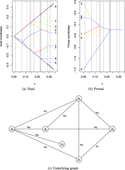
Figure 8: (a) Dual and (b) primal coordinate paths for the fused lasso applied to the graph structure shown in (c). As $\lambda$ decreases, the first dual coordinate to hit the boundary is $u_{9}$, but removing the corresponding edge does not disconnect the graph, so nothing happens in the primal setting. Then $u_{6}$ hits the boundary, and again, removing its edge does not affect the graph’s connectivity, so nothing happens. But when $u_{5}$ hits the boundary next, removing its edge disconnects the graph (the node marked $\beta_{5}$ becomes its own connected component), and hence two primal coordinate paths fuse. Note that $u_{8}$ leaves the boundary at some point (the red dashed vertical line). Adding its edge reconnects the graph, and therefore two primal coordinates unfuse.

7 A general design matrix $X$.

In the last two sections, we focused on the signal approximation case $X=I$. In this section, we consider the problem (2) when $X$ is a general $n\times p$ matrix of covariates (and $D$ is a general $m\times p$ penalty matrix). Our strategy is to again solve the equivalent dual problem (4). At first glance, this problem looks much more difficult than the dual (13) when $X=I$. Moreover, the relationship between the primal and dual solutions is now

$$\hat{\beta}_{\lambda}=(X^{T}X)^{+}(X^{T}y-D^{T}\hat{u}_{\lambda}),$$ (35)

which is also more complicated.

However, suppose that we define $\tilde{y}=XX^{+}y$ and $\widetilde{D}=DX^{+}$, where the pseudoinverse of the (rectangular) matrix $X$ is $X^{+}=(X^{T}X)^{+}X^{T}$. Abbreviating $P=P_{\mathrm{col}(X)}=XX^{+}$, the objective function in (4) becomes

$$(X^{T}y-D^{T}u)^{T}(X^{T}X)^{+}(X^{T}y-D^{T}u) = y^{T}Py-2y^{T}\widetilde{D}^{T}u+u^{T}\widetilde{D}\widetilde{D}^{T}u$$

$$= (y-\widetilde{D}^{T}u)^{T}P(y-\widetilde{D}^{T}u)$$

$$= (y-\widetilde{D}^{T}u)^{T}P^{2}(y-\widetilde{D}^{T}u)$$

$$= (\tilde{y}-\widetilde{D}^{T}u)^{T}(\tilde{y}-\widetilde{D}^{T}u).$$

The first equality above is by the definition of $D$; the second holds because $P\widetilde{D}^{T}=\widetilde{D}^{T}$; the third is because $P$ is idempotent; and the fourth is again due to the identity $P\widetilde{D}^{T}=\widetilde{D}^{T}$. Therefore we can rewrite the dual problem (4) in terms of our transformed data and penalty matrix:

$$\operatorname{minimize}\limits_{u\in\mathbb{R}^{m}}\frac{1}{2}\|\tilde{y}-\widetilde{D}^{T}u\|_{2}^{2}$$

(36)

$$\eqntext{\mbox{subject to }\|u\|_{\infty}\leq\lambda,\ D^{T}u\in\operatorname{row}(X).}$$ (37)

It is also helpful to rewrite the relationship (35) in terms of our new variables:

$$\hat{\beta}_{\lambda}=X^{+}(\tilde{y}-\widetilde{D}^{T}\hat{u}_{\lambda}),$$ (38)

which implies that the fit is simply

$$X\hat{\beta}_{\lambda}=\tilde{y}-\widetilde{D}^{T}\hat{u}_{\lambda}.$$ (39)

Modulo the row space constraint, $D^{T}u\in\operatorname{row}(X)$, problem (7) has exactly the same form as the dual (13) studied in Section 6. In the case that $X$ has full column rank, this extra constraint has no effect, so we can treat the problem just as before. We discuss this next.

7.1 The case $\operatorname{rank}(X)=p$.

Suppose that $\operatorname{rank}(X)=p$, so $\operatorname{row}(X)=\mathbb{R}^{p}$ (note that this necessarily means $p\leq n$). Then the constraint $D^{T}u\in\operatorname{row}(X)$ is trivially satisfied for any $u$, and problem (7) is the same as problem (13) that we solved in Section 6, except with $y,D$ replaced by $\tilde{y},\widetilde{D}$, respectively. Therefore, we can apply Algorithm 2 to find a dual solution path $\hat{u}_{\lambda}$, which gives the primal solution path using (38), or the fit using (39).

Fortunately, all of the properties in Section 6.2 apply to the current setting as well. First, we know that the constructed dual path $\hat{u}_{\lambda}$ is continuous and piecewise linear, because we are using the same algorithm as before. This means that $\hat{\beta}_{\lambda}$ is also continuous and piecewise linear, since it is given by the linear transformation (38). Next, we can follow the same logic in writing out the dual fit $\widetilde{D}^{T}\hat{u}_{\lambda}$ to conclude that

$$\hat{\beta}_{\lambda}=X^{+}P_{\operatorname{null}(\widetilde{D}_{-\mathcal{B}})}\bigl{(}\tilde{y}-\lambda(\widetilde{D}_{-\mathcal{B}})^{T}s\bigr{)}$$ (40)

or

$$X\hat{\beta}_{\lambda}=P_{\operatorname{null}(\widetilde{D}_{-\mathcal{B}})}\bigl{(}\tilde{y}-\lambda(\widetilde{D}_{-\mathcal{B}})^{T}s\bigr{)}.$$ (41)

Hence, $0=\widetilde{D}_{-\mathcal{B}}X\hat{\beta}_{\lambda}=D_{-\mathcal{B}}\hat{\beta}_{\lambda}$, which means that $\hat{\beta}_{\lambda}\in\operatorname{null}(D_{-\mathcal{B}})$, as before.

Though working with equations (40) and (41) may seem complicated (as one would need to expand the newly defined variables $\tilde{y},\widetilde{D}$ in terms of $y,D$), it is straightforward to show that the general primal-dual correspondence still holds here. This is given in supp . That is: the primal path $\hat{\beta}_{\lambda}$ changes slope at the values of $\lambda$ at which the null space of $D_{-\mathcal{B}(\lambda)}$ changes. For the fused lasso on a graph $\mathcal{G}$, we indeed still get fused groups of coordinates in the primal solution, since $\hat{\beta}_{\lambda}\in\operatorname{null}(D_{-\mathcal{B}})$ implies that $\hat{\beta}_{\lambda}$ is fused on the connected components of $\mathcal{G}_{-\mathcal{B}}$. Therefore, fusions still correspond to dual coordinates hitting the boundary and disconnecting the graph, and unfusions still correspond to dual coordinates leaving the boundary and reconnecting the graph.

7.2 The case $\operatorname{rank}(X)<p$.

If $\operatorname{rank}(X)<p$, then $\operatorname{row}(X)$ is a strict subspace of $\mathbb{R}^{p}$. One easy way to avoid dealing with the constraint $D^{T}u\in\operatorname{row}(X)$ of (7) is to add an $\ell_{2}$ penalty to our original problem. That is, we consider for a fixed $\varepsilon>0$

$$\operatorname{minimize}\limits_{\beta\in\mathbb{R}^{p}}\frac{1}{2}\|y-X\beta\|_{2}^{2}+\lambda\|D\beta\|_{1}+\varepsilon\|\beta\|_{2}^{2},$$ (42)

which is the same as

$$\operatorname{minimize}\limits_{\beta}\frac{1}{2}\|y^{*}-(X^{*})\beta\|_{2}^{2}+\lambda\|D\beta\|_{1},$$

where $y^{*}=(y,0)^{T}$ and $X^{*}=\left[{X\atop\varepsilon\cdot I}\right]$. Since $\operatorname{rank}(X^{*})=p$, we can use the strategy discussed in the last section, which is just applying Algorithm 2 to a transformed problem, to find the solution path of (42). Putting aside computational concerns, it may still be preferable to study problem (42) instead of problem (2). Some reasons are:

• as $\operatorname{rank}(X)<p$, the problem (2) is no longer strictly convex and may not have a unique solution; this complicates the idea of a solution path, which can now be discontinuous with respect to $\lambda$ (see holger for a related example in the fused lasso case);

• the solution of (42) may actually outperform that of (2) in terms prediction error, analogous to the advantage of the elastic net over the lasso (see enet ).

Though adding an $\ell_{2}$ penalty is easier and, as we suggested, perhaps even desirable, we can still solve the unmodified problem (2) in the $\operatorname{rank}(X)<p$ case, by looking at its dual (7). We only give a rough sketch of the path algorithm because in the present setting the solution and its computation are more complicated.

We can rewrite the row space constraint in (7) as $D^{T}u\perp\operatorname{null}(X)$. Using the SVD of $X$, we can construct an orthogonal basis for the null space of $X$. Let $W$ be the matrix that has these basis elements in its columns. Then problem (7) is now

$$\operatorname{minimize}\limits_{u\in\mathbb{R}^{m}}\frac{1}{2}\|\tilde{y}-\widetilde{D}^{T}u\|_{2}^{2}$$

(43)

$$\eqntext{\mbox{subject to }\|u\|_{\infty}\leq\lambda,\ (DW)^{T}u=0.}$$ (44)

To find a solution path of (7.2), the KKT conditions (25) need to be modified to incorporate the new equality constraint, becoming

$$(\widetilde{D}\widetilde{D}^{T}u)_{i}-(\widetilde{D}\tilde{y})_{i}+\alpha\gamma_{i}+(DW\delta)_{i}=0\qquad\mbox{for }i=1,\ldots,m,$$

where the variables are $u,\alpha,\gamma,\delta$, subject to the same constraints as before, (26a)–(26e), and additionally $(DW)^{T}u=0$. Instead of simply using the appropriate least squares estimate at each iteration, we now need to solve for $u$ and $\delta$ together. When $\lambda=\infty$, this case be done by solving the block system

$$\left[\matrix{\displaystyle\widetilde{D}\widetilde{D}^{T}&DW\cr\displaystyle(DW)^{T}&0}\right]\left[\matrix{\displaystyle u\cr\displaystyle\delta}\right]=\left[\matrix{\displaystyle\widetilde{D}\tilde{y}\cr\displaystyle 0}\right],$$ (45)

and in future iterations the expressions are similar. Having done this, satisfying the rest of the constraints (26a)–(26e) can be done by finding the hitting and leaving times just as we did previously.

8 Computational considerations.

We discuss an efficient implementation of Algorithm 2, which gives the solution path of the signal approximation problem (12), after applying the transformation (14) from dual to primal variables. For a design with $\operatorname{rank}(X)=p$, we can modify $y$ and $X$, and then the same algorithm gives the solution path of (2), this time relying on the transformation (38) for the primal path.

At each iteration of the algorithm, the dominant work is in computing expressions of the form

$$(D_{-\mathcal{B}}(D_{-\mathcal{B}})^{T})^{+}D_{-\mathcal{B}}x$$

for some vector $x$, where $\mathcal{B}$ is the current boundary set [see equations (28) and (6.1)]. Equivalently, the complexity of each iteration is based on finding

$$\operatorname{\arg\min}\limits_{v}\Bigl{\{}\|v\|_{2}\dvtx v=\operatorname{\arg\min}\limits_{w}\|x-(D_{-\mathcal{B}})^{T}w\|_{2}\Bigr{\}},$$ (46)

the least squares solution with the smallest $\ell_{2}$ norm. In the next iteration, $D_{-\mathcal{B}}$ has either one less or one more row (depending on whether a coordinate hit or left the boundary).

We can exploit the fact that the problems (46) are highly related from one iteration to the next (our strategy that is similar to that in the LARS implementation). Suppose that when $\mathcal{B}=\varnothing$, we solve the problem (46) by using a matrix factorization (e.g., a QR decomposition). In future iterations, this factorization can be efficiently updated after a row has been deleted from or added to $D_{-\mathcal{B}}$. This allows us to compute the new solution of (46) with much less work than it would take to solve the problem from “scratch.”

Recall that $D$ is $m\times n$, and the dual variable $u$ is $m$-dimensional. Let $T$ denote the number of iterations taken by the algorithm (note that $T\geq m$, and can be strictly greater if dual coordinates leave the boundary). When $m\leq n$, we can use a QR factorization of $D^{T}$ to compute the full dual solution path in

$$O(mn^{2}+Tm^{2})$$

operations. When $m>n$, using a QR factorization of $D$ allows us to compute the full dual solution path in

$$O(m^{2}n+Tn^{2})$$

operations. The main idea behind this implementation is fairly straightforward. However, the details become somewhat complicated because we require the minimum $\ell_{2}$ norm solution (46), instead of a generic solution, to the least squares problem at each iteration. See Chapters 5 and 12 of golub for an extensive coverage of the QR decomposition.

We mention two simple points to improve practical efficiency:

• The algorithm starts at the fully regularized end of the path ($\lambda=\infty$) and works toward the unregularized solution ($\lambda=0$). Therefore, for problems in which the highly or moderately regularized solutions are the only ones of interest, the algorithm can compute part of the path and terminate early. This could end up being a large savings in practice.

• One can obtain an approximate solution path by not permitting dual coordinates to leave the boundary (achieved by setting $l_{k+1}=0$ in Step 3 of Algorithm 2). This makes $T=m$, and so computing this approximate path only requires $O(mn^{2})$ or $O(m^{2}n)$ operations when $m\leq n$ or $m>n$, respectively. This approximation can be quite accurate if the number times a dual coordinate leaves the boundary is (relatively) small. Furthermore, its legitimacy is supported by the following fact: for $D=I$, this approximate path is exactly the LARS path when LARS is run it its original (unmodified) state. We discuss this in the next section.

Finally, it is important to note that if one’s goal is to find the solution of (12) or (2) over a discrete set of $\lambda$ values, and the problem size is very large, then it is likely that our path algorithm is not the most efficient approach. The reason here is the same reason that LARS is not generally used to solve large-scale lasso problems: the set of critical points (changes in slope) in the piecewise linear solution path $\hat{\beta}_{\lambda}$ becomes very dense as the problem size increases. For solving a large problem at a fixed $\lambda$, it is preferable to use a convex optimization technique that was specifically developed for the purposes of computational efficiency. First-order methods, for example, can efficiently solve large-scale instances of (12) or (2) for $\lambda$ in a discrete set (see nesta as an example).

Another optimization method of recent interest is coordinate descent cd , which is quite efficient in solving the lasso at discrete values of $\lambda$ pco , and is favored for its simplicity. But coordinate descent cannot be used for the minimizations (12) and (2), because the penalty term $\|D\beta\|_{1}$ is not separable in $\beta$, and therefore coordinate descent does not necessarily converge. In the important signal approximation case (12), however, the dual problem (13) is separable, so coordinate descent will converge if applied to the dual. Furthermore, for various applications, the matrix $D$ is sparse and structured, which means that the coordinate-wise updates for (13) are very fast. This makes coordinate descent on the dual a promising method for solving many of the signal approximation problems from Section 2.

9 Connection to LARS.

In this section, we return to the LARS algorithm, described in the Introduction as a point of motivation for our work. We assume that $\operatorname{rank}(X)=p$ and $D=I$, so that (2) is just the standard lasso problem. Our algorithm gives the lasso path $\hat{\beta}_{\lambda}$, via the dual path $\hat{u}_{\lambda}$; another way of finding the lasso path is to use the LARS algorithm in its “lasso” mode. Since the problem is strictly convex ($X$ has full column rank), there is only one solution at each $\lambda$, so of course these two algorithms must give the same result.

In its original or unmodified state, LARS returns a different path, obtained by selecting variables in order continuously decrease the maximal absolute correlation with the residual. We refer to this as the “LARS path.” Interestingly, the LARS path can be viewed as an approximation to the lasso path (see lars for an elegant interpretation and discussion of this). In our framework, we can obtain an approximate dual solution path if we never check for dual coordinates leaving the boundary, which can be achieved by dropping Step 3 from Algorithm 2 (or more precisely, by setting $l_{k+1}=0$ for each $k$). If we denote the resulting dual path by $\tilde{u}_{\lambda}$, then this suggests a primal path

$$\tilde{\beta}_{\lambda}=(X^{T}X)^{-1}(X^{T}y-\tilde{u}_{\lambda}),$$ (47)

based on the transformation in (35). The question is: how does this approximate solution path $\tilde{\beta}_{\lambda}$ compare to the LARS path?

Figure 9 shows the two paths in question. On the left is the familiar plot of lars , showing the LARS path for the “diabetes data.” The colored dots on the $x$-axis mark when variables enter the model. The right plot shows our approximate solution path on this same data set, with vertical dashed lines marking when variables (coordinates) hit the boundary. The paths look identical, and this is not a coincidence: we can show that our approximate path, which is given by ignoring dual coordinates leaving the boundary, is equal to the LARS path in general.

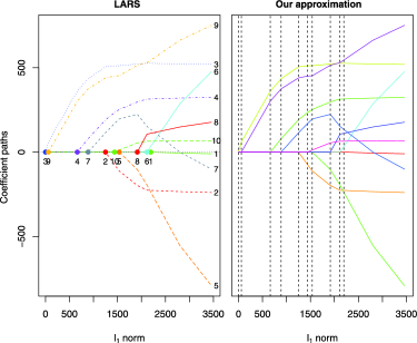
Figure 9: Comparing the LARS path and our approximate lasso path, on the diabetes data. For this data set $n=442$ and $p=10$. The paths by parametrized by the $\ell_{1}$ norm of their (respective) coefficient vectors, because the LARS path is not naturally parametrized by $\lambda$.

Lemma 2 ((Equivalence to LARS)).

Suppose that $\operatorname{rank}(X)=p$ and consider using Algorithm 2 to compute an approximate lasso path in the following way: we use $\tilde{y}=XX^{+}y$, $\widetilde{D}=X^{+}$ in place of $y,D$, and we ignore Step 3 (i.e., set $l_{k+1}=0$). Let $\tilde{u}_{\lambda}$ denote the corresponding dual path, and define a primal path $\tilde{\beta}_{\lambda}$ according to (47). Then $\tilde{\beta}_{\lambda}$ is exactly the LARS path.

First, define the residual $r_{\lambda}=y-X\tilde{\beta}_{\lambda}$. Notice that by rearranging (47), we get $\tilde{u}_{\lambda}=X^{T}r_{\lambda}$. Therefore, the coordinates of the dual path are equal to the inner products of the columns of $X$ with the current residual. This is the same as the correlations of the columns with the current residual, provided we center and scale $X$ appropriately. Hence, we have a procedure that:

• moves in a direction so that the absolute correlation with the current residual is constant within $\mathcal{B}$ (and maximal among all variables) for all $\lambda$;

• adds variables to $\mathcal{B}$ once their absolute correlation with the residual matches that realized in $\mathcal{B}$.

This almost proves that $\tilde{\beta}_{\lambda}$ is the LARS path, with $\mathcal{B}$ being the “active set” in LARS terminology. What remains to be shown is that the variables not in $\mathcal{B}$ are all assigned zero coefficients. But, recalling that $D=I$, the same arguments given in Section 6.2 and Section 7.1 apply here to give that $\tilde{\beta}_{\lambda}\in\operatorname{null}(I_{-\mathcal{B}})$ (really, $\tilde{u}_{\lambda}$ still solves a sequence of least squares problems, and the only difference between $\tilde{u}_{\lambda}$ and $\hat{u}_{\lambda}$ is in how we construct $\mathcal{B}$). This means that $\tilde{\beta}_{\lambda,-\mathcal{B}}=0$, as desired.

10 Degrees of freedom.

In general, the concept of degrees of freedom is of great interest. It describes the effective number of parameters used by a fitting procedure. This is usually easy to compute for linear procedures (linear in the data $y$) but difficult for nonlinear, adaptive procedures. In this section, we derive the degrees of freedom of the fit of problem (2), when $\operatorname{rank}(X)=p$ and $D$ is an arbitrary penalty matrix. This produces corollaries on degrees of freedom for various problems presented in Section 2. We then briefly discuss model selection using these degrees of freedom results, and last we discuss the role of shrinkage, a fundamental property of $\ell_{1}$ regularization.

10.1 Degrees of freedom results.

We assume that the data $y$ is drawn from the normal model

$$y\sim N(\mu,\sigma^{2}I),$$

and the design matrix $X$ is fixed (nonrandom). For a function $g\dvtx\mathbb{R}^{n}\rightarrow\mathbb{R}^{n}$, with $i$th coordinate function $g_{i}\dvtx\mathbb{R}^{n}\rightarrow\mathbb{R}$, the degrees of freedom of $g$ is defined as

$$\operatorname{df}(g)=\frac{1}{\sigma^{2}}\sum_{i=1}^{n}\operatorname{Cov}(g_{i}(y),y_{i}).$$

For our problem, the function of interest is $g(y)=X\hat{\beta}_{\lambda}(y)$, for fixed $\lambda$.

An alternative and convenient formula for degrees of freedom comes from Stein’s unbiased risk estimate stein . If $g$ is continuous and almost differentiable, then Stein’s formula states that

$$\frac{1}{\sigma^{2}}\sum_{i=1}^{n}\operatorname{Cov}(g_{i}(y),y_{i})=\mathrm{E}[(\nabla\cdot g)(y)].$$ (48)

Here $\nabla\cdot g=\sum_{i=1}^{n}\partial g_{i}/\partial y_{i}$ is called the divergence of $\theta$. This is useful because typically the right-hand side of (48) is easier to calculate; for our problem this is the case. But using Stein’s formula requires checking that the function is continuous and almost differentiable. In addition to checking these regularity conditions for $g(y)=X\hat{\beta}_{\lambda}(y)$, we establish below that for almost every $y$ the fit $X\hat{\beta}_{\lambda}(y)$ is a locally affine projection. Essentially, this allows us to take the divergence in (34) when $X=I$, or (41) for the general $X$ case, and treat $\mathcal{B}$ and $s$ as constants.

As in our development of the path algorithm in Sections 5, 6 and 7, we first consider the case $X=I$, because it is easier to understand. Notice that we can express the dual fit as $D^{T}\hat{u}_{\lambda}(y)=P_{C_{\lambda}}(y)$, the projection of $y$ onto the convex polytope $C_{\lambda}=\{D^{T}u\dvtx\|u\|_{\infty}\leq\lambda\}\subseteq\mathbb{R}^{n}$. From (14), the primal solution is just the residual from this projection, $\hat{\beta}_{\lambda}(y)=(I-P_{C_{\lambda}})(y)$. The projection map onto a convex set is always a contraction, and in fact, so is the residual from projecting onto a convex set (e.g., see the proof of Theorem 1.2.2 in schneider ). Therefore $\hat{\beta}_{\lambda}(y)$ is a contraction, and hence both continuous and almost differentiable (this follows from the standard proof a result called “Rademacher’s theorem;” e.g., see Theorem 2 in Section 3.2 of evans ).

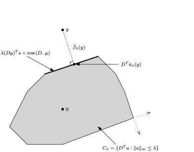
Figure 10: An illustration of the geometry surrounding $\hat{u}_{\lambda}$ and $\hat{\beta}_{\lambda}$, for the case $X=I$. Recall that $\hat{\beta}_{\lambda}(y)=y-D^{T}\hat{u}_{\lambda}(y)$, where $D^{T}\hat{u}_{\lambda}(y)$ is the projection of $y$ onto the convex polytope $C_{\lambda}=\{D^{T}u\dvtx\|u\|_{\infty}\leq\lambda\}$. Almost everywhere, small pertubations of $y$ do not change the face on which its projection lies. The exceptional set $\mathcal{N}_{\lambda}$ of points for which this property does not hold has dimension $n-1$, and is a union of rays like the two drawn as dotted lines in the bottom right of the figure.

Furthermore, thinking geometrically about the projection map onto $C_{\lambda}$ yields a crucial insight. Examine Figure 10—as drawn, it is clear that we can move the point $y$ slightly and it still projects to the same face of $C_{\lambda}$. In fact, it seems that the only points $y$ for which this property does not hold necessarily lie on rays that emanate orthogonally from the corners of $C_{\lambda}$ (two such rays are drawn leaving the bottom right corner). In other words, we are lead to believe that for almost every $y$, the projection map onto $C_{\lambda}$ is a locally constant affine projection. This is indeed true.

Lemma 3.

For fixed $\lambda$, there exists a set $\mathcal{N}_{\lambda}$ such that: [(b)]

$\mathcal{N}_{\lambda}$ has Hausdorff dimension $n-1$, hence Lebesgue measure zero;

for any $y\notin\mathcal{N}_{\lambda}$, there exists a neighborhood $U$ of $y$ such that $P_{C_{\lambda}}\dvtx U\rightarrow\mathbb{R}^{n}$ is simply the projection onto an affine subspace. In particular, the affine subspace is

$$\lambda(D_{\mathcal{B}})^{T}s+\operatorname{row}(D_{-\mathcal{B}}),$$ (49)

where $\mathcal{B}$ and $s$ are the boundary set and signs for a solution $\hat{u}_{\lambda}(y)$ of the dual problem (13),

$$\mathcal{B}=\{i\dvtx|\hat{u}_{\lambda,i}(y)|=\lambda\}\quad\mbox{and}\quad s=\operatorname{sign}(\hat{u}_{\lambda,\mathcal{B}}(y)).$$

The quantity (49) is well-defined in the sense that it is invariant under different choices of $\mathcal{B}$ and $s$ (as the dual solution may not be unique).

The proof, which follows the intuition described above, is given in supp .

Hence we have the following result.

Theorem 1.

For fixed $\lambda$, the solution $\hat{\beta}_{\lambda}$ of the signal approximation problem (12) has degrees of freedom

$$\operatorname{df}(\hat{\beta}_{\lambda})=\mathrm{E}\bigl{[}\operatorname{nullity}\bigl{(}D_{-\mathcal{B}(y)}\bigr{)}\bigr{]},$$

where the nullity of a matrix is the dimension of its null space. The expectation here is taken over $\mathcal{B}(y)$, the boundary set of a dual solution $\hat{u}_{\lambda}(y)$.

Note: Above, we can choose any dual solution at $y$ to construct the boundary set $\mathcal{B}(y)$, because by Lemma 3, all dual solutions give rise to the same $\operatorname{null}(D_{-\mathcal{B}(y)})$ (almost everywhere in $y$).

Proof of Theorem 1 Consider $y\notin\mathcal{N}_{\lambda}$, and let $\mathcal{B}$ and $s$ be the boundary set and signs of a dual solution $\hat{u}_{\lambda}(y)$. By Lemma 3, there is a neighborhood $U$ of $y$ such that

$$\hat{\beta}_{\lambda}(y^{\prime})=(I-D^{T}\hat{u}_{\lambda})(y^{\prime})=P_{\operatorname{null}(D_{-\mathcal{B}})}\bigl{(}y^{\prime}-\lambda(D_{\mathcal{B}})^{T}s\bigr{)}$$

for all $y^{\prime}\in U$. Taking the divergence at $y$ we get

$$(\nabla\cdot\hat{\beta}_{\lambda})(y)=\operatorname{tr}\bigl{(}P_{\operatorname{null}(D_{-\mathcal{B}})}\bigr{)}=\operatorname{nullity}(D_{-\mathcal{B}}),$$

since the trace of a projection matrix is just its rank. This holds for almost every $y$ because $\mathcal{N}_{\lambda}$ has measure zero, and we can use Stein’s formula to conclude that $\operatorname{df}(\hat{\beta}_{\lambda})=\mathrm{E}[\operatorname{nullity}(D_{-\mathcal{B}(y)})]$.

Now if we consider problem (2), with the design matrix satisfying$\operatorname{rank}(X)=p$, then it turns out that the same degrees of freedom formula holds for the fit $X\hat{\beta}_{\lambda}$. This is relatively straightforward to show, but requires sorting out the details of how to turn statements involving $\tilde{y},\widetilde{D}$ into those involving $y,D$. First, by the same arguments as before, we know that $X\hat{\beta}_{\lambda}(\tilde{y})$ is contracting as a function of $\tilde{y}$. But $\tilde{y}=P_{\mathrm{col}(X)}(y)$ is contracting in $y$, so indeed $X\hat{\beta}_{\lambda}(y)$ is contracting, hence continuous and almost differentiable, as a function of $y$.

Next we must establish that $\widetilde{D}^{T}\hat{u}_{\lambda}(y)$ is a locally affine projection for almost every $y$. Well, by Lemma 3, this is true of $\widetilde{D}^{T}\hat{u}_{\lambda}(\tilde{y})$ for $\tilde{y}\notin\mathcal{N}_{\lambda}$, so we have the desired result except on $\mathcal{M}_{\lambda}=(P_{\mathrm{col}(X)})^{-1}(\mathcal{N}_{\lambda})$. Following the arguments in the proof of Lemma 3, it is not hard to see that $\mathcal{N}_{\lambda}$ now has dimension $p-1$, so $\mathcal{M}_{\lambda}$ has measure zero.

With these properties satisfied, we have the following result.

Theorem 2.

Suppose that $\operatorname{rank}(X)=p$. For fixed $\lambda$, the fit $X\hat{\beta}_{\lambda}$ of the generalized lasso (2) has degrees of freedom

$$\operatorname{df}(X\hat{\beta}_{\lambda})=\mathrm{E}\bigl{[}\operatorname{nullity}\bigl{(}D_{-\mathcal{B}(y)}\bigr{)}\bigr{]},$$

where $\mathcal{B}(y)$ is the boundary set of a dual solution $\hat{u}_{\lambda}(y)$.

Note: As before, we can construct the boundary set $\mathcal{B}(y)$ from any dual solution at $y$, because the quantity $\operatorname{null}(D_{-\mathcal{B}(y)})$ is invariant (almost everywhere in $y$).

Proof of Theorem 2 Let $y\notin\mathcal{M}_{\lambda}$. We need to show that $(\nabla\cdot\break X\hat{\beta}_{\lambda})(y)=\operatorname{nullity}(D_{-\mathcal{B}(y)})$, and then applying Stein’s formula (along with the fact that $\mathcal{M}_{\lambda}$ has measure zero) gives the result.

Let $\mathcal{B}$ denote the boundary set of a dual solution $\hat{u}_{\lambda}(y)$. Then the fit is

$$X\hat{\beta}_{\lambda}(y)=P_{\operatorname{null}(\widetilde{D}_{-\mathcal{B}})}P_{\mathrm{col}(X)}y+c,$$

where $c$ denotes the terms that have zero derivative with respect to $y$. Using the fact $\operatorname{null}(X^{+})=\operatorname{null}(X^{T})$ and $\operatorname{null}(\widetilde{D}_{-\mathcal{B}})\supseteq\operatorname{null}(X^{+})$,

$$P_{\operatorname{null}(\widetilde{D}_{-\mathcal{B}})}P_{\mathrm{col}(X)} = P_{\operatorname{null}(\widetilde{D}_{-\mathcal{B}})}-P_{\operatorname{null}(\widetilde{D}_{-\mathcal{B}})}P_{\operatorname{null}(X^{+})}$$

$$= P_{\operatorname{null}(\widetilde{D}_{-\mathcal{B}})}-P_{\operatorname{null}(X^{+})}.$$

Therefore, computing the divergence:

$$\big{(}\nabla\cdot X\hat{\beta}_{\lambda}\big{)}(y) = \operatorname{nullity}(D_{-\mathcal{B}}X^{+})-\operatorname{nullity}(X^{+})$$

$$= \operatorname{nullity}(D_{-\mathcal{B}}),$$

where the last equality follows because $X$ has full column rank. This completes the proof.

We saw in Section 6.2 that the null space of $D$ has a nice interpretation for the fused lasso problem. In this case, the theorem also becomes easier to interpret.

Corollary 1 ((Degrees of freedom of the fused lasso)).

Suppose that $\operatorname{rank}(X)=p$ and that $D$ corresponds to the fused lasso penalty on an arbitrary graph. Then for fixed $\lambda$, the fit $X\hat{\beta}_{\lambda}$ of (2) has degrees of freedom

$$\operatorname{df}(X\hat{\beta}_{\lambda})=\mathrm{E}[\mbox{number of fused groups in }\hat{\beta}_{\lambda}(y)].$$

If $\mathcal{G}$ denotes the graph, we showed in Section 6.2 that the nullity of $D_{-\mathcal{B}(\lambda,y)}$ is the number of connected components in $\mathcal{G}_{-\mathcal{B}(\lambda,y)}$. We also showed (see Section 7.1 for the extension to a general design $X$) that the coordinates of $\hat{\beta}_{\lambda}(y)$ are fused on the connected components of $\mathcal{G}_{-\mathcal{B}(\lambda,y)}$, giving the result.

By slightly modifying the penalty matrix, we can derive the degrees of freedom of the sparse fused lasso.

Corollary 2 ((Degrees of freedom of the sparse fused lasso)).

Suppose that $\operatorname{rank}(X)=p$ and write $X_{i}$ for the $i$th row of $X$. Consider the sparse fused lasso problem:

$$\operatorname{minimize}\limits_{\beta\in\mathbb{R}^{p}}\sum_{i=1}^{n}(y_{i}-X_{i}^{T}\beta)^{2}+\lambda_{1}\sum_{i=1}^{p}|\beta_{i}|+\lambda_{2}\sum_{(i,j)\in E}|\beta_{i}-\beta_{j}|,$$ (50)

where $E$ is an arbitrary set of edges between nodes $\beta_{1},\ldots,\beta_{p}$. Then for fixed $\lambda_{1},\lambda_{2}$, the fit $X\hat{\beta}_{\lambda_{1},\lambda_{2}}$ of (50) has degrees of freedom

$$\operatorname{df}(X\hat{\beta}_{\lambda_{1},\lambda_{2}})=\mathrm{E}[\mbox{number of nonzero fused groups in }\hat{\beta}_{\lambda_{1},\lambda_{2}}(y)].$$

We can write (50) in the generalized lasso framework by taking $\lambda=\lambda_{2}$ and

$$D=\left[\matrix{\displaystyle D_{\mathrm{fuse}}\vspace*{3pt}\cr\displaystyle\frac{\lambda_{1}}{\lambda_{2}}I}\right],$$

where $D_{\mathrm{fuse}}$ is the fused lasso matrix corresponding to the underlying graph, with each row giving the difference between two nodes connected by an edge.

In Section 6.2, we analyzed the null space of $D_{\mathrm{fuse}}$ to interpret the primal-dual correspondence for the fused lasso. A similar interpretation can be achieved with $D$ as defined above. Let $\mathcal{G}$ denote the underlying graph and suppose that it has $m$ edges (and $p$ nodes), so that $D_{\mathrm{fuse}}$ is $m\times p$ and $D$ is $(m+p)\times p$. Also, suppose that we decompose the boundary set as $\mathcal{B}=\mathcal{B}_{1}\cup\mathcal{B}_{2}$, where $\mathcal{B}_{1}$ contains the dual coordinates in $\{1,\ldots,m\}$ and $\mathcal{B}_{2}$ contains those in $\{m+1,\ldots,m+p\}$. We can associate the first $m$ coordinates with the $m$ edges, and the last $p$ coordinates with the $p$ nodes. Then the matrix $D_{-\mathcal{B}}$ defines a subgraph $\mathcal{G}_{-\mathcal{B}}$ that can be constructed as follows: [(2)]

delete the edges of $\mathcal{G}$ that correspond to coordinates in $\mathcal{B}_{1}$, yielding $\mathcal{G}_{-\mathcal{B}_{1}}$;

keep only the nodes of $\mathcal{G}_{-\mathcal{B}_{1}}$ that correspond to coordinates in $\mathcal{B}_{2}$, yielding $\mathcal{G}_{-\mathcal{B}}$. It is straightforward to show that the nullity of $D_{-\mathcal{B}}$ is the number of connected components in $\mathcal{G}_{-\mathcal{B}}$. Furthermore, the solution $\hat{\beta}_{\lambda_{1},\lambda_{2}}(y)$ is fused on each connected component of $\mathcal{G}_{-\mathcal{B}}$ and zero in all other coordinates. Applying Theorem 2 gives the result.

The above corollary proves a conjecture of fuse , in which the authors hypothesize that the degrees of freedom of the sparse 1d fused lasso fit is equal to the number of nonzero fused coordinate groups, in expectation. But Corollary 2 covers any underlying graph, which makes it a much more general result.

By examining the null space of $D_{-\mathcal{B}}$ for other applications, and applying Theorem 2, one can obtain more corollaries on degrees of freedom. We omit the details for the sake of brevity, but list some such results in Table 2, along with those on the fused lasso for the sake of completeness. The table’s first result, on the degrees of freedom of the lasso, was already established in lassodf . The results on trend filtering and outlier detection can actually be derived from this lasso result, because these problems correspond to the case $\operatorname{rank}(D)=m$, and can be transformed into a regular lasso problem (11). For the outlier detection problem, we actually need to make a modification in order for the design matrix to have full column rank. Recall the problem formulation (8), where the coefficient vector is $(\alpha,\beta)^{T}$, the first block concerning the outliers, and the second the regression coefficients. We set $\alpha_{1}=\cdots=\alpha_{p}=0$, the interpretation being that we know a priori $p$ points $y_{1},\ldots,y_{p}$ come from the true model, and only rest of the points $y_{p+1},\ldots,y_{n}$ can possibly be outliers (this is quite reasonable for a method that simultaneous performs a $p$-dimensional linear regression and detects outliers).

=300pt Problem Unbiased estimate of $\bolds{\operatorname{df}(X\hat{\beta}_{\lambda})}$ Lasso Number of nonzero coordinates Fused lasso Number of fused groups Sparse fused lasso Number of nonzero fused groups Polynomial trend filtering, order $k$ Number of knots ${}+{}k+1$ Outlier detection Number of outliers $+{}p$

Table 2: Corollaries of Theorem 2, giving unbiased estimates of $\operatorname{df}(X\hat{\beta}_{\lambda})$ for various problems discussed in Section 2. These assume that $\operatorname{rank}(X)=p$

10.2 Model selection.

Note that the estimates in Table 2 are all easily computable from the solution vector $\hat{\beta}_{\lambda}$. The estimates for the lasso, (sparse) fused lasso, and outlier detection problems can be obtained by simply counting the appropriate quantity in $\hat{\beta}_{\lambda}$. The estimate for trend filtering may be difficult to determine visually, as it may be difficult to identify the knots in a piecewise polynomial by eye, but the knots can counted from the nonzeros of $D\hat{\beta}_{\lambda}$. All of this is important because it means that we can readily use model selection criteria like $C_{p}$ or BIC for these problems, which employ degrees of freedom to assess risk. For example, for the estimate $X\hat{\beta}_{\lambda}$ of the underlying mean $\mu$, the $C_{p}$ statistic is

$$C_{p}(\lambda)=\|y-X\hat{\beta}_{\lambda}\|_{2}^{2}-n\sigma^{2}+2\sigma^{2}\,\operatorname{df}(X\hat{\beta}_{\lambda}),$$

and is an unbiased estimate of the true risk $\mathrm{E}[\|\mu-X\hat{\beta}_{\lambda}\|_{2}^{2}]$. Hence, we can define

$$\widehat{C}_{p}(\lambda)=\|y-X\hat{\beta}_{\lambda}\|_{2}^{2}-n\sigma^{2}+2\sigma^{2}\operatorname{nullity}(D_{-\mathcal{B}}),$$

replacing $\operatorname{df}(X\hat{\beta}_{\lambda})$ by its own unbiased estimate $\operatorname{nullity}(D_{-\mathcal{B}})$. This modified statistic $\widehat{C}_{p}(\lambda)$ is still unbiased as an estimate of the true risk, and this suggests choosing $\lambda$ to minimize $\widehat{C}_{p}(\lambda)$. For this task, it turns out that $\widehat{C}_{p}(\lambda)$ obtains its minimum at one of the critical points $\{\lambda_{1},\ldots,\lambda_{T}\}$ in the solution path of $\hat{\beta}_{\lambda}$. This is true because $\operatorname{nullity}(D_{-\mathcal{B}})$ is a step function over these critical points, and the residual sum of squares $\|y-X\hat{\beta}_{\lambda}\|_{2}^{2}$ is monotone nondecreasing for $\lambda$ in between critical points [this can be checked using (41)]. Therefore, Algorithm 2 can be used to simultaneously compute the solution path and select a model, by simply computing $\widehat{C}_{p}(\lambda_{k})$ at each iteration $k$.

10.3 Shrinkage and the $\ell_{1}$ norm.

At first glance, the results in Table 2 seem both intuitive and unbelievable. For the fused lasso, for example, we are told that on average we spend a single degree of freedom on each group of coordinates in the solution. But these groups are being adaptively selected based on the data, so aren’t we using more degrees of freedom in the end? As another example, consider the trend filtering result: for a cubic fit, the degrees of freedom is the number of knots $+{}4$, in expectation. A cubic regression spline also has degrees of freedom equal to the number of knots $+{}4$; however, in this case we fix the knot locations ahead of time, and for cubic trend filtering the knots are selected automatically. How can this be?

This seemingly remarkable property—that searching for the nonzero coordinates, fused groups, knots, or outliers does not cost us anything in terms of degrees of freedom—is explained by the shrinking nature of the $\ell_{1}$ penalty. Looking back at the criterion in (2), it is not hard to see that the nonzero entries in $D\hat{\beta}_{\lambda}$ are shrunken toward zero (imagine the problem in constrained form, instead of Lagrange form). For the fused lasso, this means that once the groups are “chosen,” their coefficients are shrunken towards each other, which is less greedy than simply fitting the group coefficients to minimize the squared error term. Roughly speaking, this makes up for the fact that we chose the fused groups adaptively, and in expectation, the degrees of freedom turns out “just right”: it is simply the number of groups.

This leads us to think about the $\ell_{0}$-equivalent of problem (2), which is achieved by replacing the $\ell_{1}$ norm by an $\ell_{0}$ norm (giving best subset regression when $D=I$). Solving this problem requires a combinatorial optimization, and this makes it difficult to study the properties of its solution in general. However, we do know that the solution of the $\ell_{0}$ problem does not enjoy any shrinkage property like that of the lasso solution: if we fix which entries of $D\beta$ are nonzero, then the penalty term is constant and the problem reduces to an equality-constrained regression. Therefore, in light of our above discussion, it seems reasonable to conjecture that the $\ell_{0}$ fit has more than $\mathrm{E}[\operatorname{nullity}(D_{-\mathcal{B}})]$ degrees of freedom. When $D=I$, this would mean that the degrees of freedom of the best subset regression fit is more than the number of nonzero coefficients, in expectation.

11 Discussion.

We have studied a generalization of the lasso problem, in which the penalty is $\|D\beta\|_{1}$ for a matrix $D$. Several important problems (such as the fused lasso and trend filtering) can be expressed as a special case of this, corresponding to a particular choice of $D$. We developed an algorithm to compute a solution path for this general problem, provided that the design matrix $X$ has full column rank. This is achieved by instead solving the (easier) Lagrange dual problem, which, using simple duality theory, yields a solution to the original problem after a linear transformation.

Both the dual solution path and the original solution path are continuous and piecewise linear with respect to $\lambda$. The original solution $\hat{\beta}_{\lambda}$ can be written explicitly in terms of the boundary set $\mathcal{B}$, which contains the coordinates of the dual solution that are equal to $\pm\lambda$, and the signs of these coordinates $s$. Furthermore, viewing the dual solution as a projection onto a convex set, we derived a simple formula for the degrees of freedom of the generalized lasso fit. This formula emphasizes the importance of the dual perspective, as it is fundamentally tied to the boundary set $\mathcal{B}$. For the fused lasso problem, this result reveals that the number of nonzero fused groups in the solution is an unbiased estimate of the degrees of freedom of the fit, and this holds true for any underlying graph structure. Other corollaries follow, as well.

An implementation of our path algorithm, following the ideas presented in Section 8, is a direction for future work, and will be made available as an R package “genlasso” on the CRAN website cran . There are several other directions for future research. We describe three possibilities below.

• Specialized implementation for the fused lasso path algorithm. When $D$ is the fused lasso matrix corresponding to a graph $\mathcal{G}$, projecting onto the null space of $D_{-\mathcal{B}}$ is achieved by a simple coordinate-wise average on each connected component of $\mathcal{G}_{-\mathcal{B}}$. It may therefore be possible to compute the solution path $\hat{\beta}_{\lambda}$ without having to use any linear algebra, but by instead tracking the connectivity of $\mathcal{G}$. This could improve the computational efficiency of each iteration, and could also lead to a parallelized approach (in which we work on each connected component in parallel).

• Number of steps until termination. The number of steps $T$ taken by our path algorithm, for a general $D$, is determined by how many times dual coordinates leave the boundary. This is related to an interesting problem in geometry studied by donoho , and investigating this connection could lead to a more definitive statement about the algorithm’s computational complexity.

• Connection to forward stagewise regression. When $D=I$, we proved that our path algorithm yields the LARS path (when LARS is run in its original, unmodified state) if we simply ignore dual coordinates leaving the boundary. LARS can be modified to give forward stagewise regression, which is the limit of forward stepwise regression when the step size goes to zero (see lars ). A natural follow-up question is: can our algorithm be changed to give this path too?

We believe that Lagrange duality deserves more attention in the study of many convex optimization problems in statistics. The dual problem can often have a complementary (and interpretable) structure, which can offer both computational benefits and novel mathematical or statistical insights into the original problem.

Acknowledgments.

The authors thank Robert Tibshirani for his many interesting suggestions and great support. Nick Henderson and Michael Saunders provided valuable input with the computational considerations. We also thank Trevor Hastie for his help with the LARS algorithm. Finally, we thank the referees and especially the Editor for all of their help making this paper more readable.

Proofs and technical details [doi]10.1214/11-AOS878SUPP .pdf aos878_suppl.pdf A supplementary document that contains a number of proofs and technical details concerning “The solution path of the generalized lasso.”

References

- (1) {barticle}[auto:STB—2010-11-18—09:18:59] \bauthor\bsnmBecker, \bfnmS.\binitsS., \bauthor\bsnmBobin, \bfnmJ.\binitsJ. and \bauthor\bsnmCandes, \bfnmE. J.\binitsE. J. (\byear2011). \btitleNESTA: A fast and accurate first-order method for sparse recovery. \bjournalSIAM Journal on Imaging Sciences \bvolume4 \bpages1–39. \endbibitem
- (2) {bbook}[auto:STB—2010-11-18—09:18:59] \bauthor\bsnmBertsekas, \bfnmD. P.\binitsD. P. (\byear1999). \btitleNonlinear Programming. \bpublisherAthena Scientific, \baddressNashua, NH. \endbibitem
- (3) {bmisc}[auto:STB—2010-11-18—09:18:59] \bauthor\bsnmBest, \bfnmM. J.\binitsM. J. (\byear1982). \bhowpublishedAn algorithm for the solution of the parametric quadratic programming problem. CORR Report 82–84, Univ. Waterloo. \endbibitem
- (4) {bbook}[mr] \bauthor\bsnmBoyd, \bfnmStephen\binitsS. and \bauthor\bsnmVandenberghe, \bfnmLieven\binitsL. (\byear2004). \btitleConvex Optimization. \bpublisherCambridge Univ. Press, \baddressCambridge. \bidmr=2061575 \endbibitem
- (5) {barticle}[pbm] \bauthor\bsnmBredel, \bfnmMarkus\binitsM., \bauthor\bsnmBredel, \bfnmClaudia\binitsC., \bauthor\bsnmJuric, \bfnmDejan\binitsD., \bauthor\bsnmHarsh, \bfnmGriffith R.\binitsG. R., \bauthor\bsnmVogel, \bfnmHannes\binitsH., \bauthor\bsnmRecht, \bfnmLawrence D.\binitsL. D. and \bauthor\bsnmSikic, \bfnmBranimir I.\binitsB. I. (\byear2005). \btitleHigh-resolution genome-wide mapping of genetic alterations in human glial brain tumors. \bjournalCancer Res. \bvolume65 \bpages4088–4096. \bidpii=65/10/4088, doi=10.1158/0008-5472.CAN-04-4229, pmid=15899798 \endbibitem
- (6) {bmisc}[auto:STB—2010-11-18—09:18:59] \borganizationCenters for Disease Control and Prevention. (\byear2009). \bhowpublished“Novel H1N1 flu situation update.” Available at http://www.cdc.gov/h1n1flu/updates/061909.htm. \endbibitem
- (7) {barticle}[mr] \bauthor\bsnmChen, \bfnmScott Shaobing\binitsS. S., \bauthor\bsnmDonoho, \bfnmDavid L.\binitsD. L. and \bauthor\bsnmSaunders, \bfnmMichael A.\binitsM. A. (\byear1998). \btitleAtomic decomposition by basis pursuit. \bjournalSIAM J. Sci. Comput. \bvolume20 \bpages33–61. \biddoi=10.1137/S1064827596304010, mr=1639094 \endbibitem
- (8) {bincollection}[auto:STB—2010-11-18—09:18:59] \bauthor\bsnmCleveland, \bfnmW.\binitsW., \bauthor\bsnmGrosse, \bfnmE.\binitsE., \bauthor\bsnmShyu, \bfnmW.\binitsW. and \bauthor\bsnmTerpenning, \bfnmI.\binitsI. (\byear1991). \btitleLocal regression models. In \bbooktitleStatistical Models in S (\beditorJ. Chambers and T. Hastie, eds.). \bpublisherWadsworth, \baddressBelmont, CA. \endbibitem
- (9) {barticle}[mr] \bauthor\bsnmDonoho, \bfnmDavid L.\binitsD. L. and \bauthor\bsnmJohnstone, \bfnmIain M.\binitsI. M. (\byear1995). \btitleAdapting to unknown smoothness via wavelet shrinkage. \bjournalJ. Amer. Statist. Assoc. \bvolume90 \bpages1200–1224. \bidmr=1379464 \endbibitem
- (10) {barticle}[mr] \bauthor\bsnmDonoho, \bfnmDavid L.\binitsD. L. and \bauthor\bsnmTanner, \bfnmJared\binitsJ. (\byear2010). \btitleCounting the faces of randomly-projected hypercubes and orthants, with applications. \bjournalDiscrete Comput. Geom. \bvolume43 \bpages522–541. \biddoi=10.1007/s00454-009-9221-z, mr=2587835 \endbibitem
- (11) {barticle}[mr] \bauthor\bsnmEfron, \bfnmBradley\binitsB., \bauthor\bsnmHastie, \bfnmTrevor\binitsT., \bauthor\bsnmJohnstone, \bfnmIain\binitsI. and \bauthor\bsnmTibshirani, \bfnmRobert\binitsR. (\byear2004). \btitleLeast angle regression. \bjournalAnn. Statist. \bvolume32 \bpages407–499. \biddoi=10.1214/009053604000000067, mr=2060166 \bptnotecheck related \endbibitem
- (12) {barticle}[mr] \bauthor\bsnmElad, \bfnmMichael\binitsM., \bauthor\bsnmMilanfar, \bfnmPeyman\binitsP. and \bauthor\bsnmRubinstein, \bfnmRon\binitsR. (\byear2007). \btitleAnalysis versus synthesis in signal priors. \bjournalInverse Problems \bvolume23 \bpages947–968. \biddoi=10.1088/0266-5611/23/3/007, mr=2329926 \endbibitem
- (13) {bbook}[mr] \bauthor\bsnmEvans, \bfnmLawrence C.\binitsL. C. and \bauthor\bsnmGariepy, \bfnmRonald F.\binitsR. F. (\byear1992). \btitleMeasure Theory and Fine Properties of Functions. \bpublisherCRC Press, \baddressBoca Raton, FL. \bidmr=1158660 \endbibitem
- (14) {barticle}[mr] \bauthor\bsnmFriedman, \bfnmJerome\binitsJ., \bauthor\bsnmHastie, \bfnmTrevor\binitsT., \bauthor\bsnmHöfling, \bfnmHolger\binitsH. and \bauthor\bsnmTibshirani, \bfnmRobert\binitsR. (\byear2007). \btitlePathwise coordinate optimization. \bjournalAnn. Appl. Statist. \bvolume1 \bpages302–332. \biddoi=10.1214/07-AOAS131, mr=2415737 \endbibitem
- (15) {bbook}[mr] \bauthor\bsnmGolub, \bfnmGene H.\binitsG. H. and \bauthor\bsnmVan Loan, \bfnmCharles F.\binitsC. F. (\byear1996). \btitleMatrix Computations, \bedition3rd ed. \bpublisherJohns Hopkins Univ. Press, \baddressBaltimore, MD. \bidmr=1417720 \endbibitem
- (16) {barticle}[mr] \bauthor\bsnmHastie, \bfnmTrevor\binitsT., \bauthor\bsnmRosset, \bfnmSaharon\binitsS., \bauthor\bsnmTibshirani, \bfnmRobert\binitsR. and \bauthor\bsnmZhu, \bfnmJi\binitsJ. (\byear2003/04). \btitleThe entire regularization path for the support vector machine. \bjournalJ. Mach. Learn. Res. \bvolume5 \bpages1391–1415 (electronic). \bidmr=2248021 \bptnotecheck year \endbibitem
- (17) {bbook}[mr] \bauthor\bsnmHastie, \bfnmT.\binitsT. and \bauthor\bsnmTibshirani, \bfnmR.\binitsR. (\byear1990). \btitleGeneralized Additive Models. \bseriesMonographs on Statistics and Applied Probability \bvolume43. \bpublisherChapman & Hall, \baddressLondon. \bidmr=1082147 \endbibitem
- (18) {barticle}[mr] \bauthor\bsnmHastie, \bfnmTrevor\binitsT. and \bauthor\bsnmTibshirani, \bfnmRobert\binitsR. (\byear1993). \btitleVarying-coefficient models. \bjournalJ. Roy. Statist. Soc. Ser. B \bvolume55 \bpages757–796. \bidmr=1229881 \bptnotecheck related \endbibitem
- (19) {bmisc}[auto:STB—2010-11-18—09:18:59] \bauthor\bsnmHoefling, \bfnmH.\binitsH. (\byear2009). \bhowpublishedA path algorithm for the fused lasso signal approximator. Unpublished manuscript. Available at http://www.holgerhoefling.com/ Articles/FusedLasso.pdf. \endbibitem
- (20) {barticle}[mr] \bauthor\bsnmJames, \bfnmGareth M.\binitsG. M., \bauthor\bsnmRadchenko, \bfnmPeter\binitsP. and \bauthor\bsnmLv, \bfnmJinchi\binitsJ. (\byear2009). \btitleDASSO: Connections between the Dantzig selector and lasso. \bjournalJ. R. Stat. Soc. Ser. B Stat. Methodol. \bvolume71 \bpages127–142. \biddoi=10.1111/j.1467-9868.2008.00668.x, mr=2655526 \endbibitem
- (21) {barticle}[mr] \bauthor\bsnmKim, \bfnmSeung-Jean\binitsS.-J., \bauthor\bsnmKoh, \bfnmKwangmoo\binitsK., \bauthor\bsnmBoyd, \bfnmStephen\binitsS. and \bauthor\bsnmGorinevsky, \bfnmDimitry\binitsD. (\byear2009). \btitle trend filtering. \bjournalSIAM Rev. \bvolume51 \bpages339–360. \biddoi=10.1137/070690274, mr=2505584 \endbibitem
- (22) {barticle}[mr] \bauthor\bsnmOsborne, \bfnmMichael R.\binitsM. R., \bauthor\bsnmPresnell, \bfnmBrett\binitsB. and \bauthor\bsnmTurlach, \bfnmBerwin A.\binitsB. A. (\byear2000). \btitleOn the LASSO and its dual. \bjournalJ. Comput. Graph. Statist. \bvolume9 \bpages319–337. \biddoi=10.2307/1390657, mr=1822089 \endbibitem
- (23) {bmisc}[auto:STB—2010-11-18—09:18:59] \borganizationR Development Core Team (\byear2008). \bhowpublishedR: A Language and Environment for Statistical Computing. R Foundation for Statistical Computing, Vienna, Austria. Available at http://www.R-project.org. \endbibitem
- (24) {barticle}[mr] \bauthor\bsnmRosset, \bfnmSaharon\binitsS. and \bauthor\bsnmZhu, \bfnmJi\binitsJ. (\byear2007). \btitlePiecewise linear regularized solution paths. \bjournalAnn. Statist. \bvolume35 \bpages1012–1030. \biddoi=10.1214/009053606000001370, mr=2341696 \endbibitem
- (25) {barticle}[auto:STB—2010-11-18—09:18:59] \bauthor\bsnmRudin, \bfnmL. I.\binitsL. I., \bauthor\bsnmOsher, \bfnmS.\binitsS. and \bauthor\bsnmFaterni, \bfnmE.\binitsE. (\byear1992). \btitleNonlinear total variation based noise removal algorithms. \bjournalPhys. D \bvolume60 \bpages259–268. \endbibitem
- (26) {bbook}[mr] \bauthor\bsnmSchneider, \bfnmRolf\binitsR. (\byear1993). \btitleConvex Bodies: The Brunn–Minkowski Theory. \bseriesEncyclopedia of Mathematics and Its Applications \bvolume44. \bpublisherCambridge Univ. Press, \baddressCambridge. \biddoi=10.1017/CBO9780511526282, mr=1216521 \endbibitem
- (27) {barticle}[mr] \bauthor\bsnmShe, \bfnmY.\binitsY. (\byear2010). \btitleSparse regression with exact clustering. \bjournalElectron. J. Stat. \bvolume4 \bpages1055–1096. \bidmr=2727453 \endbibitem
- (28) {bmisc}[auto:STB—2010-11-18—09:18:59] \bauthor\bsnmShe, \bfnmY.\binitsY. and \bauthor\bsnmOwen, \bfnmA. B.\binitsA. B. (\byear2010). \bhowpublishedOutlier detection using nonconvex penalized regression. Unpublished manuscript. Available at http://www-stat.stanford.edu/ ~owen/reports/theta-ipod.pdf. \endbibitem
- (29) {barticle}[mr] \bauthor\bsnmStein, \bfnmCharles M.\binitsC. M. (\byear1981). \btitleEstimation of the mean of a multivariate normal distribution. \bjournalAnn. Statist. \bvolume9 \bpages1135–1151. \bidmr=0630098 \endbibitem
- (30) {barticle}[mr] \bauthor\bsnmTibshirani, \bfnmRobert\binitsR. (\byear1996). \btitleRegression shrinkage and selection via the lasso. \bjournalJ. Roy. Statist. Soc. Ser. B \bvolume58 \bpages267–288. \bidmr=1379242 \endbibitem
- (31) {barticle}[mr] \bauthor\bsnmTibshirani, \bfnmRobert\binitsR., \bauthor\bsnmSaunders, \bfnmMichael\binitsM., \bauthor\bsnmRosset, \bfnmSaharon\binitsS., \bauthor\bsnmZhu, \bfnmJi\binitsJ. and \bauthor\bsnmKnight, \bfnmKeith\binitsK. (\byear2005). \btitleSparsity and smoothness via the fused lasso. \bjournalJ. R. Stat. Soc. Ser. B Stat. Methodol. \bvolume67 \bpages91–108. \biddoi=10.1111/j.1467-9868.2005.00490.x, mr=2136641 \endbibitem
- (32) {bmisc}[vtex] \bauthor\bsnmTibshirani, \bfnmRyan J.\binitsR. J. and \bauthor\bsnmTaylor, \bfnmJonathan\binitsJ. (\byear2011). \bhowpublishedSupplement to “The solution path of the generalized lasso” DOI:10.1214/11-AOS878SUPP. \endbibitem
- (33) {barticle}[mr] \bauthor\bsnmTseng, \bfnmP.\binitsP. (\byear2001). \btitleConvergence of a block coordinate descent method for nondifferentiable minimization. \bjournalJ. Optim. Theory Appl. \bvolume109 \bpages475–494. \biddoi=10.1023/A:1017501703105, mr=1835069 \endbibitem
- (34) {barticle}[mr] \bauthor\bsnmZou, \bfnmHui\binitsH. and \bauthor\bsnmHastie, \bfnmTrevor\binitsT. (\byear2005). \btitleRegularization and variable selection via the elastic net. \bjournalJ. R. Stat. Soc. Ser. B Stat. Methodol. \bvolume67 \bpages301–320. \biddoi=10.1111/j.1467-9868.2005.00503.x, mr=2137327 \endbibitem
- (35) {barticle}[mr] \bauthor\bsnmZou, \bfnmHui\binitsH., \bauthor\bsnmHastie, \bfnmTrevor\binitsT. and \bauthor\bsnmTibshirani, \bfnmRobert\binitsR. (\byear2007). \btitleOn the “degrees of freedom” of the lasso. \bjournalAnn. Statist. \bvolume35 \bpages2173–2192. \biddoi=10.1214/009053607000000127, mr=2363967 \endbibitem