The Clumping Transition in Niche Competition:
a Robust Critical Phenomenon

Abstract

We show analytically and numerically that the appearance of lumps and gaps in the distribution of $n$ competing species along a niche axis is a robust phenomenon whenever the finiteness of the niche space is taken into account. In this case depending if the niche width of the species $\sigma$ is above or below a threshold $\sigma_{c}$, which for large $n$ coincides with $\frac{2}{n}$, there are two different regimes. For $\sigma>\sigma_{c}$ the lumpy pattern emerges directly from the dominant eigenvector of the competition matrix because its corresponding eigenvalue becomes negative. For $\sigma\leq\sigma_{c}$ the lumpy pattern disappears. Furthermore, this clumping transition exhibits critical slowing down as $\sigma$ is approached from above. We also find that the number of lumps of species vs. $\sigma$ displays a stair-step structure. The positions of these steps are distributed according to a power-law. It is thus straightforward to predict the number of groups that can be packed along a niche axis and it coincides with field measurements for a wide range of the model parameters.

1 Introduction

An important problem in ecology is how closely can species be packed in a natural environment [1]. A usual way to approach this issue is by considering the species distributed along a hypothetical one-dimensional niche axis [1]. To fix ideas one may consider the niche axis as a gradient that is related to the size of organisms. Each species $i$ is represented by a normal distribution $P_{i}$($\xi$)= $\exp$ [-($\xi-\mu_{i})^{2}$/2$\sigma^{2}$ ] centered at $\mu_{i}$, corresponding to its average position $\xi$ on this niche axis, and with a standard deviation $\sigma$, which measures the width of its niche. The competition for finite resources among the $n$ species can be described by a Lotka-Volterra competition model (LVCM):

$$\frac{dN_{i}}{dt}=r_{i}\frac{N_{i}}{K_{i}}(K_{i}-\sum_{j=1}^{n}a_{ij}N_{j}),$$ (1)

where $N_{i}$ is the density of species $i$, $r_{i}$ is its maximum per-capita growth rate, $K_{i}$ is the carrying capacity of species $i$ and the coefficients $a_{ij}$ is the competition coefficient of species $j$ on species $i$. It seems natural to assume that the intensity of the interaction between two species $i$ and $j$ depends on how close they are along the niche axis. A measure of this is provided by the niche overlap, ı.e. the overlapping between $P_{i}(\xi)$ and $P_{j}(\xi)$. The competition coefficients $a_{ij}$ can be computed by the MacArthur and Levins overlap (MLO) formula [2]:

$$a_{ij}=\frac{\int_{-\infty}^{\infty}P_{i}(\xi)P_{j}(\xi)d\xi}{\int_{-\infty}^{\infty}P_{i}^{2}(\xi)}=\mbox{e}^{-(\frac{\mu_{i}-\mu_{j}}{2\sigma})^{2}}.$$ (2)

Recently Scheffer and van Nes [3] found by simulations that the combination of LVCM (1) plus MLO (2) yields long transients of lumpy distributions of species along the niche axis [For asymptotic times, the lumps are thinned out to single species unless a stabilizing mechanism/term is included, as it was shown in [3].]

This phenomenon of spontaneous emergence of self-organized clusters of look-a-likes separated by gaps with no survivors was dubbed by the authors as self-organized similarity (SOS). It was recognized as an important new finding in an established model in ecology [4, 5] In addition, there is empirical evidence for self-organized coexistence of similar species in communities ranging from mammal [6] and bird communities [7] to lake plankton [8].

However, there has been some controversy on whether this lumpy distribution of species is indeed a robust result or rather depends strongly on details of the model, like the competition kernel [9, 10].

Here we show that the lumpy pattern is a robust phenomenon provided one takes into account the finiteness of the niche axis. Thus, truncation besides being a crucial assumption which guarantees clustering, allows the analytical computation of the eigenvalues and eigenvectors of the competition matrix A with elements $a_{ij}$ given by (2). Furthermore, we show that ultimately solving the linear problem is enough to get both the transient pattern -lumps and gaps between them- as well as the asymptotic equilibrium. The plan of this work is as follows:

Since an analytic solution for realistic conditions - species randomly distributed along a finite and non periodic niche axis, each with a different per capita growth rate $r_{i}$ and carrying capacity $K_{i}$ - is not possible, we will consider in section 2 a series of simplifications. We get an analytic expression for the state of this simpler system, in terms of the dominant eigenvector of A. It provides a qualitatively good description of the system for not too short times and becomes very good for asymptotic times. Part of the material of this section was presented in a previous short paper [11], but there are some important differences like considering a less rough approximation together with some steps better explained.

In section 3 we show, using simulations, that all these simplifications do not destroy SOS: lumps and gaps remain in the case of a finite linear niche axis no matter if the niche is non periodic (i.e. it has borders), or the species are randomly distributed, or $r$ and $K$ changes from species to species. Indeed we go further and show that SOS occurs in niches of more than one dimensions or when interaction kernels different from the Gaussian kernel are considered.

In section 4 we show that the prediction of the number of lumps as a function of $\sigma$ is in good agreement with measures in several ecosystems [1], provided $\sigma$ is greater than a threshold value $\sigma_{c}$. For this critical value it occurs a bifurcation which is responsible for the clumping transition.

Section 5 is devoted to conclusions and to put our results in its proper perspective, addressing some general concerns about SOS and comparing with other different approaches.

2 AN ANALYTICAL PROOF OF SELF-ORGANIZED SIMILARITY IN A SIMPLIFIED CASE

We start by considering the following simplifications:

S1 - The $n$ species are evenly distributed along a finite niche axis of length $L$ = 1, i.e. $\mu_{i}$ = $(i\!-\!1)/n$ ($i$=1,…,$n$).

S2 - To avoid border effects, the niche is defined circular, i.e. periodic boundary conditions (PBC) are imposed. This is done by just taking the smallest of $|$$\mu_{i}$-$\mu_{j}$$|$ and 1-$|$$\mu_{i}$-$\mu_{j}$$|$ as the distance between the niche centers.

S3 - All species have the same per capita growth rate which we take equal to 1, $r_{i}$ = 1 for all $i$.

S4 - The carrying capacity $K$ is also homogeneous, $K_{i}$ = $K$ for all $i$.

Under the simplifying conditions S3 and S4 the system of equations (1) reduces to

$$\frac{dx_{i}}{dt}=x_{i}(1-\sum_{j=1}^{n}a_{ij}x_{j}),$$ (3)

where $x_{i}$ is the density of species $i$, normalized by its carrying capacity $K_{i}$ ($x_{i}$ = $N_{i}/K_{i}$).

An equilibrium of the system (3)is specified by a set of densities $x_{i}^{*}$, one for each species $i$, verifying:

$$x_{i}^{*}(1-\sum_{j=1}^{n}a_{ij}x_{j}^{*})=0.$$ (4)

A standard procedure to check the stability of this equilibrium is linear stability analysis. That is, to consider, initially small, disturbances $y_{i}(0)$ from the equilibrium values $x_{i}^{*}$ and study their fate $y_{i}(t)$ as the time grows. Let’s take $x_{i}^{*}=x^{*}\forall i$ which, by virtue of conditions S1 and S2, is an exact equilibrium . The evolution equation for $y_{i}(t)$ can be written as

$$\frac{dy_{i}}{dt}=-(x^{*}+y_{i}(t))\sum_{j=1}^{n}a_{ij}y_{j}(t).$$ (5)

Since the coefficients of the matrix A given by (2) are symmetric, in the eigenvector basis $\{\mbox{{\bf v}}_{i}\}$, it becomes diagonal with all its eigenvalues $\lambda_{i}$ real. Hence integrating equation (5) , and using that $y_{i}(0)$ is small, $y_{i}(t)$ can be approximated by

$$y_{i}(t)\simeq y_{i}(0)e^{-x^{*}\lambda_{i}t}.$$ (6)

Thus, for asymptotic times, y becomes proportional to the dominant eigenvector v^m, the one associated with the minimum eigenvalue of A, $\lambda_{m}$, i.e.

$$\mbox{\bf y}(t)\propto e^{-x^{*}\lambda_{m}t}\mbox{\bf v}^{m}\;\;\;\mbox{(for large times)}.$$ (7)

We will show that, for a wide range of the parameters $n$ and $\sigma$, $\lambda_{m}$($n$,$\sigma$) is in general negative (see below). Hence, from (7), y is amplified over time instead of decaying to zero (as it would happen in the case of a positive $\lambda_{m}$). Therefore, for large times, from (5) we can express the time derivative of x as

$$\frac{d\mbox{\bf x}}{dt}=-\mbox{\bf x}(t)\lambda_{m}\mbox{\bf v}^{m},$$ (8)

and by integration we get the approximated solution given by

$$\mbox{\bf x}\approx e^{-\lambda_{m}\mbox{\bf v}^{m}t}\;\;\;\mbox{(for large times)}.$$ (9)

Analytic expressions for the eigenvalues and eigenvectors of A are not known for the general case of random distributions of species on a niche axis with arbitrary boundary conditions. However, for the simpler case when the $n$ species are evenly spaced along the niche axis, $\mu_{j}$ = $(j\!-\!1)/n$ (with the index $j$=1,…,$n$), and PBC (the simplifying conditions S1 and S2) A becomes a matrix whose rows are cyclic permutations of the first one:

$$\begin{bmatrix}c_{1}&c_{2}&\dots&c_{n-1}&c_{n}\\ c_{n}&c_{1}&\dots&c_{n-2}&c_{n-1}\\ \dots&\dots&\dots&\dots&\dots\\ \dots&\dots&\dots&\dots&\dots\\ c_{2}&c_{3}&\dots&c_{n}&c_{1}\end{bmatrix}$$

with $c_{j}(n,\sigma)=e^{-(\frac{\widetilde{j-1}}{2\sigma n})^{2}}$, where the tilde stands for $\pmod{\frac{n+2}{2}}$ implementing then PBC. For this case, the eigenvalues $\lambda_{k}$ and the components of the eigenvectors $v^{k}$ ($k$ = 1,…,$n$) are given by [12]:

$$\lambda_{k}=\sum_{j=1}^{n}c_{j}(n,\sigma)e^{i2\pi(k-1)\mu_{j}}$$

$$=\sum_{j=1}^{n}c_{j}(n,\sigma)e^{i2\pi(k-1)(j-1)/n},$$ (10)

and

$$v_{j}^{k}=n^{-\frac{1}{2}}[\cos(2\pi(k\!-\!1)\mu_{j})+\sin(2\pi(k\!-\!1)\mu_{j})]$$

$$=n^{-\frac{1}{2}}\left[\cos\left(\frac{2\pi(k\!-\!1)(j\!-\!1)}{n}\right)+\sin\left(\frac{2\pi(k\!-\!1)(j\!-\!1)}{n}\right)\right].$$ (11)

Since the matrix A is symmetric $c_{j}=c_{n+2-j}$. Therefore, from (10) one can see that the eigenvalues occur in pairs: $\lambda_{k}=\lambda_{n-k}$, with the exception of $\lambda_{1}$ (and of $\lambda_{n/2+1}$ if $n$ is even). Furthermore, these paired eigenvalues can be expressed as

$$\lambda_{k}=2\sum_{j=2}^{n/2}c_{j}(n,\sigma)\cos[2\pi(k-1)(j-1)/n].\\$$ (12)

Equation (10) can be used to determine the index $k$ = $m$ that gives the minimal eigenvalue, for $n$ and $\sigma$ given, $\lambda_{m}(n,\sigma)$ (as we have just seen, the index $k$ = $n$-$m$+2 produces the same value). The surface depicted in Fig. 1 corresponds to $\lambda_{m}$($n$,$\sigma$) computed for a grid 2$\leq$ $n$ $\leq$ 200, and 0.05 $\leq$ $\sigma$ $\leq$ 0.5. Notice that $\lambda_{m}$ is negative except for small values of $\sigma$ and becomes positive when $n$ $<$ 8.

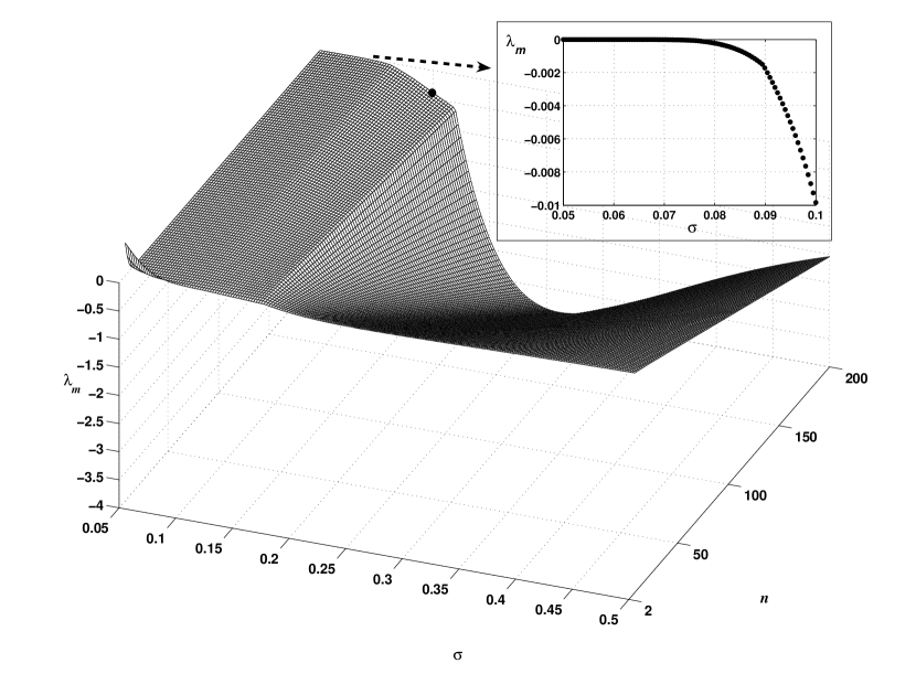
Figure 1: The minimal eigenvalue of A, $\lambda_{m}$ , determined from equation 10, as a function of $n$ and $\sigma$. The black spot denotes the point $n$ = 200 and $\sigma$ = 0.15. Inset: a zoom of $\lambda_{m}$ vs. $\sigma$ for $n$ = 200 in the interval 0.05 $\leq\sigma\leq$ 0.1.

The substitution of the dominant eigenvector v^m, which from (11) has $m$-1 peaks and $m$-1 valleys, into (9) allows to predict the distribution of species for long enough times.

The results we got were checked by numerical simulations. In these simulations the initial values for the $x_{i}$ are random numbers between 0 and 1. Then the system of differential equations (ODE) is integrated for a given final time. In Fig. 2 we compare this analytical approximation with simulations. For instance, if $n$ = 200 and $\sigma$ = 0.15 we get $m$ = 5 ( and $m$ = 200-5+2 = 197), $\lambda_{m}$ = 0.3938 and the components of v^m are given by $\sqrt{\frac{1}{n}}\sin[8\pi\mu_{j}]$ + $\sqrt{\frac{1}{n}}\cos[8\pi\mu_{j}]$. Panel (A) of Fig.2 if for $t$ =1000 generations. The agreement is quite good and the quality of the agreement improves with time, until it becomes very good when the lumps are thinned to single lines as it is shown in panel (B). This happens because we are not considering any lump stabilizing term like the one considered in [3]. Notice that ultimately the lumps and gaps coincide, respectively, with the $m$ -1 maximums and minimums of v^m.

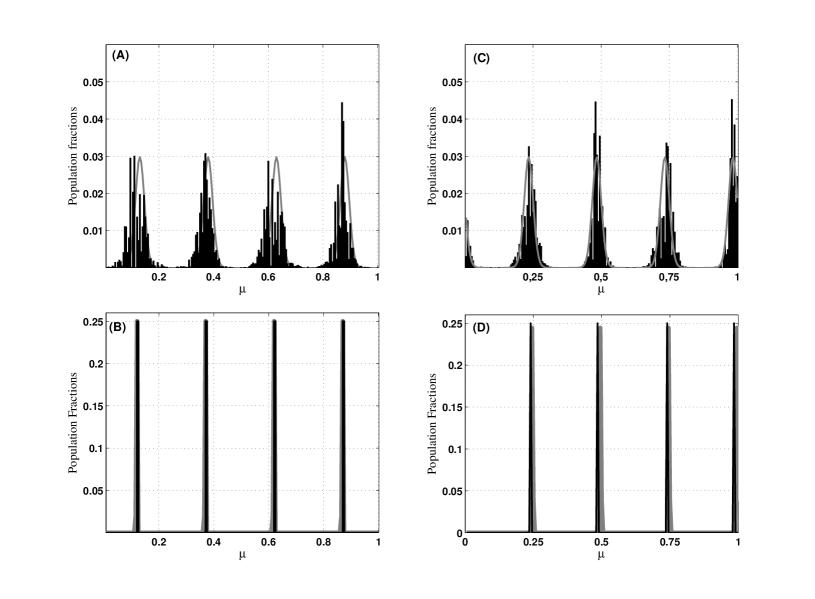
Figure 2: Population fractions $\hat{x}_{i}$ for $n$ = 200 and $\sigma$ = 0.15. In black results from a simulation after $t$ generations and in gray $\exp$ [ -$\lambda_{m}$v^m $t$]. (A) and (B): Species evenly spaced along the niche axis for $t$ = 1000 and $t$ = 10,000 generations, respectively. (C) and (D): Species randomly distributed along the niche axis for $t$ = 1000 and $t$ = 10,000.

The integer $m$, which gives the minimal eigenvalue, is a function of the width $\sigma$ of the niche, $m$ = $m$($\sigma$). It does not depend from $n$ provided $n$ is large enough. Nevertheless, as we will show in section IV, $m$ becomes a function of $n$ and $\sigma$ for small values of both these parameters. For example, for $\sigma$=0.15, $m$-1 = 4 for all even $n$ greater or equal than 8. This lower $n$ limit arises because the maximum possible number of peaks that can be accommodated with $n$ vector components is $n$/2 (one half of the components of v^m pointing up and the other half down). So in this particular case $n$/2 must be greater or equal than 4, and, in general, $n$/2 must be greater or equal than $m$-1.

Another remarkable result about $m$ is that it is always an odd number (and then the number of clumps is even). The reason for this can be traced from the cosines appearing in (12) making contributions to the eigenvalues of opposite signs: positive for odd $k$ and negative for even $k$. As a consequence the number of peaks, equal to $m$-1, is always even.

3 SELF-ORGANIZED SIMILARITY PERSISTS UNDER MORE REALISTIC ASSUMPTIONS

In order to consider more realistic assumptions, abandoning the simplifying conditions S1-S4, we rely in the following exclusively on simulations. Since the emphasis in SOS is on transient maintenance of clumps of similar species, one might wonder about how initial conditions determine the results, and how species that are being driven extinct ever managed to get up to high density in the first place. So, as before, the ODE system is integrated starting from initial $x_{i}$ which are random numbers between 0 and 1. We checked in all the cases that changes in the initial populations don’t introduce qualitative changes.

1. From evenly to randomly distributed species.

What happens in the general case of randomly distributed species over the niche axis? In this case the spectrum and v^m are obtained numerically from A. It turns out that simulations produce quite the same results. We illustrate this in Fig.2 where we plot the population fractions normalized to one, $\hat{x}_{i}=\frac{x_{i}}{\sum_{i=1}^{n}x_{i}}$, for the particular parameter values $n$=200 and $\sigma$=0.15. The resemblance is clear when comparing panels (C) and (D) with, respectively, (A) and (B). In fact, the spectrum of eigenvalues in both cases is very similar as it is shown in Table 1 (the values on the right correspond to averages among simulations).

	Evenly spaced	Randomly distributed
$\lambda_{1}$	-0.3938	-0.4 $\pm$0.01
$\lambda_{2}$	-0.3938	-0.4 $\pm$0.01
⋮	⋮	⋮
$\lambda_{198th}$	45.391	46$\pm$0.96
$\lambda_{199th}$	45.391	46$\pm$0.96
$\lambda_{200th}$	104.387	105 $\pm$1.93

Table 1: eigenvalues of A for $n$ = 200 & $\sigma$ = 0.15 ordered from small to large i.e. $\lambda_{m}=\lambda_{1}=\lambda_{2}$.

2. Taking into account border effects in a linear niche axis.

We also analyzed what happens when a linear, instead of a circular niche axis (PBC), of length $L$ is considered. The competition coefficients for these open boundary conditions (OBC) are now given by

$$a_{ij}=\mbox{e}^{-(\frac{\mu_{i}-\mu_{j}}{2\sigma})^{2}}\frac{\mbox{erf}(\frac{2L\!-\!\mu_{i}\!-\!\mu_{j}}{2\sigma})+\mbox{erf}(\frac{\mu_{i}\!+\!\mu_{j}}{2\sigma})}{\mbox{erf}(\frac{L\!-\!\mu_{i}}{\sigma})+\mbox{erf}(\frac{\mu_{i}}{\sigma})}.$$ (13)

When using competition coefficients given by (13) with $L$=1, again, a lumpy pattern emerges although it shows some quantitative differences. For example, a four lump pattern occurs for smaller values of $\sigma$, e.g. $\sigma$= 0.12 instead of $\sigma$= 0.15 (panel (A) in Fig.3). Additionally, although $\lambda_{m}$ is still negative, due to the factor multiplying the Gaussian in (13), the matrix A is no longer symmetric and so there appear complex eigenvalues.

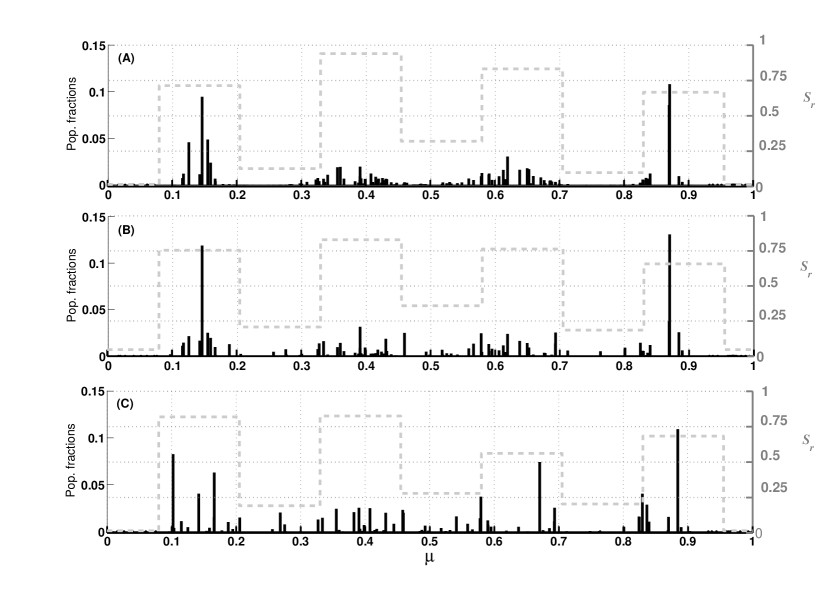
Figure 3: Fraction of species $\hat{x}_{i}$ (black bars, left vertical axis) for $n$ = 200, $\sigma$ = 0.1 and open boundary conditions (coefficients given by (13) with $L$=1) after 500 generations and the corresponding entropy for each lump and gap region $S_{r}$ (gray dashed lines, right vertical axis). (A): Uniform maximum growth rate $r$ and carrying capacity $K$. (B): Varying $r$ (the $r_{i}$ are random numbers with average value equal to 1) and uniform $K$. (C): Varying $r$ (the $r_{i}$ are random numbers with average value equal to 1) and $K$ ( $\delta K_{max}/\bar{K}$ = 0.2, see text) from species to species.

3. The effect of a non uniform growth rate.

Simplification S3 was to consider a uniform $r$. Indeed it is simple to realize that an $r$ varying from species to species does not introduce major changes. This is because what is relevant for the equilibrium values $x_{i}^{*}$ are the terms between brackets in the LVCM equations (see panel (B) in Fig.3).

4. The effect of the heterogeneity in the carrying capacity.

We find that when variations $\pm$$\delta$$K_{i}$ of the carrying capacity around an average value $\bar{K}$ occur in such a way that the amplitude of these fluctuations, $\delta$$K_{max}$, is no greater than 10 % of $\bar{K}$ the lumpy pattern changes but is similar to the one corresponding to the homogeneous case. If, in addition, one assumes that the carrying capacity of neighbor species along the niche axis have similar carrying capacities and larger variations are only possible for species which are far away on the niche axis, then larger values of $\delta$$K_{max}$/$\bar{K}$ still preserve SOS (panel (C) in Fig.3). On the other hand, strong random variations of the carrying capacity along the niche axis in general destroy the SOS pattern.

In Fig.3 we show the population fractions obtained when the more realistic conditions 2 to 4 are gradually taken into account. In the three panels we plot the results produced by simulations starting from the same initial distribution of populations. Panel (A) corresponds to OBC and homogeneous $r$ and $K$, panel (B) to OBC, heterogeneous $r$ and homogeneous $K$ and panel (C) to OBC and heterogeneous $r$ as well as $K$. Notice that although the lumpy structure becomes less clear as the original restrictions are lifted, it is still recognizable in panel (C). In order to provide a more quantitative test for the clumping to the favorable niches, it is necessary to introduce an observable which measures species coexistence or diversity. Among the different indices proposed to measure species diversity perhaps the most common is the Shannon-Wiener index [13],[14], or in the physics language the well known entropy $S$, defined by

$$S=-\sum_{i=1}^{n}\hat{x}_{i}\ln\hat{x}_{i}.$$

Moreover, entropy analysis has been used to quantify species diversity and niche breadth [15] and to recognize ecological structures (see [16] and references therein). Therefore we proceed as follows. From the homogeneous $r$ and $K$ situation we obtain the modulation along the niche axis determining the number and positions of lumps and gaps. In this specific case there are four lumps separated by gaps all of the same length. Thus we divide the niche axis into 9 regions: 4 lumps and 3 gaps between them, all the 7 of length 0.125, plus the two smaller gaps at the niche borders completing the remaining length of 0.125. The amount of entropy $S_{r}$ calculated for each region ($r$=1,2,…), measures the species diversity (represented by gray dashed lines in panels (A)-(C)). Notice that the profile of $S_{r}$ for the three situations is similar although, as expected, it offers more clear cut evidence of lumps and gaps for the homogeneous situation of panel (A): the entropy is in general lower (higher) at the gaps (lumps of coexistence) than in panels (B) or (C). Therefore, we conclude that the considered simplifications don’t introduce substantial changes and that SOS survives in more realistic conditions.

Other competition kernels and multidimensional niches

It was argued that the formula (2) is a special case and that competition coefficients are typically non-Gaussian [9, 17]. Some recent analyses explore more general non-Gaussian competition kernels of the form [18]:

$$a_{ij}=\mbox{e}^{-(\frac{\mu_{i}-\mu_{j}}{2\sigma})^{p}},$$ (14)

which reduces to the Gaussian one for $p$=2. Moreover, it was claimed that Gaussian competition does not lead to patterns but is a borderline case between patterns and non-patterns regimes [10]. However, this depends on whether or not one takes into account the finiteness of the niche axis. When it is taken into account, as we do by using a truncated kernel, $p$=2 is no longer a border case. Rather the lumpy pattern occurs for any real kernel exponent $p$ above 1, for example, $p$ = 1.5 as is it is shown in panel (A) of Fig. 4 for $\sigma$=0.19. This is because the only change in the formula for the eigenvalues (10) is in the coefficients $c_{j}(n,\sigma)$ which, for a general value of the exponent $p$, are given by $c_{j}(n,\sigma)=e^{-(\frac{j-1}{2\sigma n})^{p}}$ while the expression (11) for the eigenvectors remains unchanged. Panel (B) of this figure is a plot of the components of the v^m showing that its peaks (valleys) coincide with the lumps (gaps).

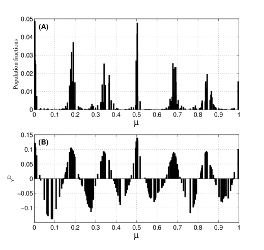
Figure 4: Results for a non-Gaussian kernel with $p$=1.5, $n$ = 200, $\sigma$ = 0.19 and PBC. (A): Distribution of species for after 2500 generations. (B): Components of the dominant eigenvector v^m.

Another common criticism is that it is not very realistic to consider a one-dimensional niche, rather niches (utilizations) in general are multi-dimensional [19, 20] It turns out that a multi-dimensional niche only makes the math a little bit less straightforward. Suppose that the $n$ species are distributed at random in a 2-dimensional niche with axes $\mu_{1}$ and $\mu_{2}$. Then one can assign an index $i$ to each population, located at the point in niche space given by a couple ($\mu_{1i}$,$\mu_{2i}$), and group them into a vector of $n$ components. Therefore, the expression for the competition coefficient between species $i$, located in this niche space at a point of coordinates ($\mu_{1i}$,$\mu_{2i}$), and species $j$, at ($\mu_{1j}$,$\mu_{2j}$), can be written as

$$a_{ij}=\mbox{e}^{-\frac{(\mu_{1i}-\mu_{1j})^{2}+(\mu_{2i}-\mu_{2j})^{2}}{(2\sigma)^{2}}}.$$ (15)

It turns out that this preserves the cyclic property of the A matrix - its rows are cyclic permutations of the first one -, a property required to get the expressions for the eigenvalues (10) and the eigenvectors (11) [12]. Fig. 5 shows the results for $\sigma$=0.2. It shows a general result we found: if in the case of a one-dimensional niche ($d$=1), for a given value of $\sigma$, there are $m$-1 lumps, for a two-dimensional niche ($d$=2) there occur ($m$-1)$\times$($m$-1) lumps (for $\sigma$ = 0.2 there are 2 lumps for $d$=1 while for $d$=2 there are 4 lumps).

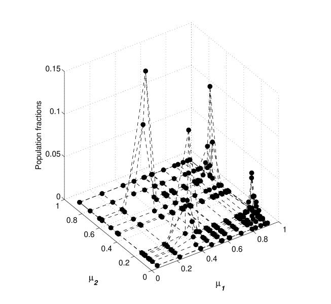
Figure 5: Distribution of species in a two-dimensional niche of coordinate axis $\mu_{1}$ and $\mu_{2}$ for $n$ = 15$\times$15= 225 species, and $\sigma$ = 0.2, PBC after 100 generations. 2$\times$2=4 clumps are observable.

4 THE DEPENDENCE OF CLUMPING ON THE NICHE WIDTH AND THE CLUMPING TRANSITION

How close species can be packed along the niche axis is commonly measured by the parameter $d/\sigma$, where $d$ is the separation between species [1]. In the case of the model under consideration, $d$ can either measure the separation between a) lumped groups of species, persisting during long transients or b) surviving species (one per lump), for asymptotic times. So we get either an estimate for the species packing or for the group packing. In any event, this distance coincides with the inverse of the number of peaks of v^m, which depends on $\sigma$, and is given by $n_{\infty}$ ($\sigma$) = $m$($\sigma$)-1. Fig.6 shows $n_{\infty}$ for $\sigma$ ranging from 0.05 to 0.5 and the number of species fixed to $n$ = 200. There is a series of steps, located at values $\sigma_{s}$, that become wider as $\sigma_{s}$ increases. The height of these steps is always 2. This is because, as we have seen in section 2, the number of peaks of v^m is always an even number. That is, if $\sigma_{s}^{-}$ ($\sigma_{s}^{+}$) corresponds to $\sigma$ tending to $\sigma_{s}$ by the left (right), then $n_{\infty}$($\sigma_{s}^{-}$) = $n_{\infty}$($\sigma_{s}^{+}$)+2. For example, if $\sigma$ $>$ $\sigma_{s}$ $\simeq$ 0.169 then v^m has always 2 peaks, below this value the number of its peaks jumps to 4, and so on. We find that when $\sigma$ tends to $\sigma_{s}^{+}$ , $n_{\infty}$ can be fitted with the power-law 0.09$\sigma_{s}^{-1.75}$ (dashed line in Fig.6). The packing parameter in the different step regions can be approximated, by taking the number of peaks at each $\sigma_{s}$ as the semi-sum of the numbers of peaks at each side of the step, as:

$$\frac{d}{\sigma_{s}}\simeq\frac{1}{\sigma_{s}1/2(n_{\infty}(\sigma_{s}^{+})+n_{\infty}(\sigma_{s}^{-}))}=\frac{1}{\sigma_{s}+0.09\sigma_{s}^{-0.75}}.$$ (16)

This quotient varies from approximately 1.96 for the first step, at $\sigma_{s}$ $\simeq$0.169, to 1.1 for the last step, at $\sigma_{s}$ $\simeq$ 0.05. This is in good agreement with many field measurements that found a species packing ratio always lying between 1 and 2 [1].

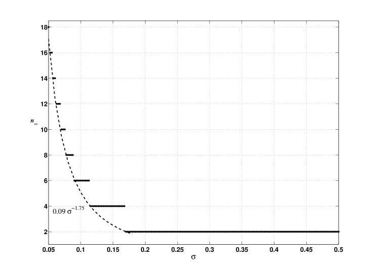
Figure 6: Number peaks $n_{\infty}$ of the dominant eigenvector v^m as a function of $\sigma$ ($n$ = 200). The jumps follow a power-law distribution indicated by a dashed line.

It is worth remarking that when $\sigma$ decreases, $\lambda_{m}$ -which is in general negative- increases, until at some critical value, $\sigma_{c}$, it becomes 0. That is, in Thom’s catastrophe theory language [21], a degenerate critical point or a Non-Morse critical point. This $\sigma_{c}$ depends on the number of species: it decreases with $n$. We computed $\sigma_{c}(n)$ as the values such that $\lambda_{m}(n,\sigma_{c})$ becomes 0. In Fig.7 we show this. Notice that for $n\geq 40$ $\sigma_{c}$ scales as 2$n^{-1}$, i.e. the double of the initial average separation between species. As $\sigma$ is decreased in simulations -for a fixed value of $n$- so that it becomes closer and closer to $\sigma_{c}$ and $\lambda_{m}$ moves towards 0, we observed that the time to reach the lumpy pattern grows unbounded. This is the well known phenomenon of critical slowing down[22] : the characteristic relaxation time of the dominant eigenmode is proportional to 1/$\lambda_{m}$. In fact, taking $n$=200, for $\sigma$ = 0.15 the 4 lumps are noticeable after typically 500 generations while the 6 lumps for $\sigma$ = 0.1 require around 20,000 generations and for $\sigma$ = 0.075 it takes a huge number of generations (more than 500,000) to produce the 10 lumps pattern. The inset of Fig.1 is a zoom of $\lambda_{m}$ vs. $\sigma$. It shows that, at least for all practical purposes, the clumping becomes noticeable at $\sigma\simeq$ 0.075.

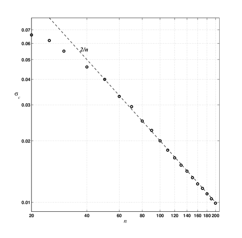
Figure 7: Log-log plot of $\sigma_{c}$ vs. $n$ for $n$ between 20 and 200. The dashed line corresponds to 2/$n$.

5 CONCLUSIONS AND FINAL COMMENTS

A realistic mathematical description of the dynamics of a large number of species placed along a resource spectrum is a complicated issue for which an exact solution is not available. In fact, analytical work looks at the long-term equilibria of models. The alternative to deal with the transients are simulations.

However a simulation approach, like the one used by Scheffer and van Nes [3] may leave room for doubts on whether things might be artifacts. We made a series of simplifications which allow an analytic proof, by working directly with the community matrix A, of the emergence of SOS. Roughly, the lumpy pattern one is seeing is the exponential of the dominant eigenvector v^m of A (multiplied by the time).

We later have shown that this is indeed a robust result. The clumping phenomenon does not depend on the boundary conditions nor on the kernel exponent $p$ (provided it is greater than one), it is quite independent on the heterogeneity of species parameters $r$ and $K$, it occurs for a wide range of $\sigma$, and in more than one niche dimensions. In addition, Roelke and Eldridge [23] found similar patterns in a different resource competition model. They also suggest that this mechanism is not very fragile. Additional supporting evidences can be found in [24].

A crucial element to get clumping is to take into account the finiteness of the niche axis. This, besides being realistic, leads to a $\lambda_{m}$ with a negative real part (and then to lumps and gaps). We want to remark that either OBC or the standard implementation of PBC imply a niche which is finite. This explains remarkable differences with the outcomes reported in [10]. The procedure they use to implement PBC consists in taking a periodic array of copies of the same system. This “perfectly periodic” boundary conditions mimic an infinite niche axis. The first of such differences is that, in our case, the SOS is robust against variations on the kernel: a negative $\lambda_{m}$ is obtained whenever the exponent $p$ of the kernel interaction is a real number greater than 1. The second difference, is that the parameter $\sigma$, controlling the width of each species distribution, plays a fundamental role. There is a critical value, $\sigma_{c}$, below which there is no clustering. On the other hand, in a virtually infinite niche axis, since it is always possible to set $\sigma$ = 1 by rescaling $\mu$, the clustering should not depend on $\sigma$. However it seems natural that things in ecosystems depend on $\sigma$, and usually the interest is precisely in measuring this effect. This is another powerful reason to prefer an implementation of boundary conditions like the one we are using.

Similar approaches to determine pattern formation in phenotype space have also been used by Levin and Segel [25], Sasaki [26] and more recently by Meszéna and co-workers [27],[28]. The main difference of our approach is that a discrete set of phenotypes is considered, instead of a continuum. This is an important feature, since firstly it can affect the assessment concerning how robust SOS is. That is, in the case of a continuous set of phenotypes, it was shown that an arbitrarily small perturbation can destroy the continuous coexistence making the species distribution discrete [27],[28]. And this could be taken as an evidence of the breaking of SOS. On the other hand, in our model, from the very beginning, the distribution of species is discrete and SOS it is rather understood as a strong overlap of the species distributions. Secondly, it allows to go beyond the large $n$ limit and applying it to real communities, involving a number of species $n$ of intermediate size. For example, this was tested for the case of phytoplankton communities in a lake ecosystem involving between 50 to 100 species and the agreement between theory and empirical data is quite good [29]. Moreover, in this real ecosystem the fact that $\sigma$ is not the same for all species, rather varies from species to species, doesn’t spoil the lumpy pattern.

There are interesting parallels with similar phenomena in physical systems:

• For example, the fact that the emergence of the lumpy pattern is related to the eigenvector with the minimum eigenvalue and the number of lumps is determined mostly by the model parameter $\sigma$ resembles the spinodal decomposition That is, under the spinodal decomposition the system develops a spatially modulated order parameter whose amplitude grows continuously from zero and extend throughout the entire system. This results in domains of a characteristic length scale called the spinodal length $\lambda_{sp}$ which usually depends strongly on temperature (because the second derivative of the free energy becomes increasingly negative deep inside the region delimited by the spinodal) [30].

• The emergence of power laws and critical slowing down are attractive ingredients to physicists since they are signatures of self-organized criticality (SOC) [31]. This tendency to spontaneously self-organize into a critical state, without any significant “tuning” of some control parameter, usually reflects a share of the same fundamental dynamics for many different systems referred to as universality. While the origin of critical slowing down is clear explained by the existence of a degenerate critical point, the power law distribution for the plateaus of the number of lumps vs. $\sigma$ is not completely understood and deserves further analysis.

• The application of techniques and concepts of statistical mechanics into very different realms like ecosystems might be of interest to ecologists, statistical physicists and to the growing community on the intersection of both fields. In that sense, the analytical proof of clumping is based on statistical mechanics results from Berlin and Kac [12] when they were analysing the spherical model of a ferromagnet.

• The calculation of the entropy for different regions of a system, to get an overview about the level of correlation between elements in each region has been used in several contexts closer to physics. For example: cellular automata [32], deterministic models of nonlinear dynamics [33], glass-forming materials [34], astrophysics of galaxies and clusters [35], image processing [36], to mention some. In our case it has shown to be useful to identify the lumpy structure.

To conclude, it is remarkable that the predictions on the number of groups of species that can be packed along the niche axis are quantitatively consistent with field data for a wide range of values of both the width of the niche and the number of species.

References

References

- [1] May R. M. Stability and Complexity in Model Ecosystems. Princeton University Press, 1974.
- [2] MacArthur R. H. and Levins R. The limiting similarity, convergence, and divergence of coexisting species. Am. Nat., 101:377–385, 1967.
- [3] Scheffer M. and van Nes E. Self-organized similarity, the evolutionary emergence of groups of similar species. Proc. Natl. Acad. Sci. USA, 103:6230–6235, 2006.
- [4] Nee S. and Colegrave N. Paradox of the clumps. Nature, 441:417–418, 2006.
- [5] May R. M., Crawley J. M. and Sugihara G. Theoretical Ecology Principles and Applications. Oxford University Press, 2007.
- [6] Siemann E. and Brown J. H. Gaps in mammalian body size distributions reexamined. Ecology, 80:2788–2792, 1999.
- [7] Holling C. S. Cross-scale morphology, geometry and dynamics of ecosystems. Ecol. Monogr., 62:447–502, 1992.
- [8] Havlicek T. D. and Carpenter S. R. Pelagic species size distributions in lakes: Are they discontinuous? Oceanogr., 46:1021–1033, 2001.
- [9] Abrams P. A. and Rueffler C. Competition similarity relationships, and the nonlinearity of competitive effects in consumer-resource systems. Am. Nat., 172:463–474, 2008.
- [10] Pigolotti S., López C. and Hernández-García E. Species clustering in competitive lotka-volterra models. Phys. Rev. Lett., 98:258101–04, 2007.
- [11] Fort H., Scheffer M. and van Nes E. The paradox of the clumps mathematically explained. Theoretical Ecology, 2:171–176, 2009.
- [12] Berlin T. H. and Kac M. The spherical model of a ferromagnet. Phys. Rev., 86:821–835, 1952.
- [13] Pielou E. C. Introduction to Mathematical Ecology. Wiley-Interscience, New York, 1969.
- [14] Hill M. O. Diversity and evenness: A unifying notation and its consequences. Ecology, 54:427–432, 1973.
- [15] Egerton F.N. History of American Ecology. Arno Press, 1977.
- [16] Pineda F. D. et al. Ecological structures recognized by means of entropy analysis: assessment of differences between entropy values. J. Theor. Biol., 135:283–293, 1988.
- [17] Wilson D. S. The adequacy of body size as a niche difference. Am. Nat., 109:769–784, 1975.
- [18] Doebeli M. et al. Multimodal pattern formation in phenotype distributions of sexual populations. Proc. Biol. Sci., 274:347–357, 2001.
- [19] Schoener T. W. Resource partitioning in ecological communities. Science, 185:27–39, 1974.
- [20] Pacala S. and Roughgarden J. The evolution of resource partitioning in a multidimensional resource space. Theor. Pop. Biol., 22:127–145, 1982.
- [21] Thom R. Structural Stability and Morphogenesis. Reading, Benjamin, 1975.
- [22] Gilmore R. Catastrophe Theory for Scientists and Engineers. Dover, 1981.
- [23] Roelke D. L. and Eldridge P. M. Mixing of supersaturated assemblages and the precipitous loss of species. Am. Nat., 171:162–175, 2008.
- [24] Herault B. Reconciling niche and neutrality through the emergent group approach. Evolution and Systematics, 9:71, 2007.
- [25] Levin S. A. and Segel L. A. Pattern generation in space and aspect. SIAM Review, 27:45–67, 1985.
- [26] Sasaki A. Clumped distribution by neighborhood competition. J. Theor. Biol., 186:415–430, 1997.
- [27] Barabás G. and Meszéna G. When the exception becomes the rule: the disappearance of limiting similarity in the lotka-volterra model. J. Theor. Biol., 258:89–94, 2009.
- [28] Szabó P. and Meszéna G. Limiting similarity revisited. Oikos, 112:663–724, 2006.
- [29] Fort H. and Segural A. Self-organized similarity: Theoretical and empirical results. to be published elsewhere, 2010.
- [30] Papon P., Leblond J. and Meijer P. The Physics of Phase Transitions: Concepts and Applications. Springer, 2006.
- [31] Bak P. How nature works : the science of self-organized criticality. Copernicus, New York, USA, 1996.
- [32] Mitchel M., Crutchfield J. P. and Hraber P. T. Dynamics, computation, and the “edge of chaos”: A re-examination. In Cowan G., Pines D. and D. Melzner, editors, Complexity: Metaphors, Models, and Reality. Santa Fe Institute Stuides in the Sciences of Complexity, Proceedings Volume 19., pages 497–513. Reading, MA: Addison-Wesley, 1994.
- [33] Diambra L. Maximum entropy approach to nonlinear modeling. Physica A, 278:140–149, 2000.
- [34] Murthy S. S. N. Strength and fragility in glass-forming liquids. J. Phys. Chem., 93:3347–3351, 1989.
- [35] Voit G. M. et al. On the origin of intracluster entropy. Astroph. Jour., 593:272–290,, 2003.
- [36] Bakhtiari A. S. et al. An efficient segmentation method based on local entropy characteristics of iris biometrics. World Academy of Science, Engineering and Technology, 28:64–68, 2007.