Two species coagulation approach to consensus by group level interactions

Abstract

We explore the self-organization dynamics of a set of entities by considering the interactions that affect the different subgroups conforming the whole. To this end, we employ the widespread example of coagulation kinetics, and characterize which interaction types lead to consensus formation and which do not, as well as the corresponding different macroscopic patterns. The crucial technical point is extending the usual one species coagulation dynamics to the two species one. This is achieved by means of introducing explicitly solvable kernels which have a clear physical meaning. The corresponding solutions are calculated in the long time limit, in which consensus may or may not be reached. The lack of consensus is characterized by means of scaling limits of the solutions. The possible applications of our results to some topics in which consensus reaching is fundamental, like collective animal motion and opinion spreading dynamics, are also outlined.

I Introduction

The property that characterizes those systems which long range order is due to the coupling of simple interactions at their different scales is usually denoted as emergence. It has been studied in many different contexts, ranging from collective animal motion couzin to linguistic dynamics cucker and passing through condensed matter escudero and financial systems lux . It is thus a fundamental property of many important systems which encodes essential information about them. Emergence is commonly studied as arising directly from the interactions of the most fundamental units configuring the system. However, self-organization does not necessarily happen this way. Macroscopic order may be a consequence of interactions at different scales, in which the diverse subsystems play a particular contributing role. We will illustrate how this occurs by means of studying the dynamics of particular coagulation equations. While the origins and consequences of the arising of consensus by group level interactions go far beyond the use of coagulation equations, these constitute a reasonable approach to the subject, precisely due to their universality. Indeed, coagulation equations have proved their utility in topics as diverse as aerosols seinfeld , polymerization ziff , Ostwald ripening ls ; meerson , galaxies and stars clustering silk , and population biology niwa among many others. They thus exemplify the broad applicability that the understanding of this sort of ordering processes may bring.

A classical example of self-organizing systems is collective organism behavior, which has been studied using a broad range of theoretical techniques bertozzi ; bodnar ; orsogna . This includes the adaptation of some of the classical models of statistical mechanics of spin systems vicsek . Indeed, statistical physics models and methods have been successfully adapted to situations of a completely different nature such as opinion formation and spreading toral ; fortunato . One of the classical models in this context is the voter model voter1 ; voter2 ; liggett , which has been studied within both fields of statistical mechanics and probability theory. Due to the large generality in which these and similar processes appear it seems appealing extending coagulation models to two species dynamics. On one hand, the extension is natural from a methodological viewpoint; on the other hand, it smoothly matches with previous approaches in the subject of self-organization. Clustering has been previously studied in population dynamics models emilio including swarming systems clusterswarm , and coagulation equations have been used in both swarming coaguswarm and opinion formation models toral2 . We shall show in the following how two-species coagulation may constitute a sensible extension of previous approaches.

There exist many biological examples of collective motion, including insects, birds, fishes… In these cases the interaction among individuals gives rise to a consensus which consists in the selection of the direction of motion. A specific example that has been extensively studied both from the experimental and theoretical point of view is the problem of locusts swarming. The experiment performed in buhl revealed that locusts marching on a (quasi one dimensional) ring presented a coherent collective motion for high densities; low densities were characterized by a random behavior of the individuals and intermediate densities showed coherent displacements alternating with sudden changes of direction. The models that have been introduced to describe this experiment assume that the organisms behave like interacting particles buhl ; yates . Related interacting particle models have been used to describe the collective behavior of many different organisms and analyzing the mathematical properties of such models is currently a very active research area bertozzi ; orsogna ; vicsek .

In this paper we will not try to describe the detailed behavior of any specific organism. Our goal will be to explore the mathematical consequences of models of organism clustering, that is an alternative way of describing the collective behavior of these systems. This approach does not rule out the possibility of particle-like interactions among the components of the system, but it assumes that the tendency to follow the behavior of the neighborhoods is strong enough to produce collective effects at the level of the whole cluster instead of individual elements. As we shall see, this experiment suggests interesting two-species coagulation dynamics. We also expect that our approach may be of some relevance in the field of opinion formation, again as an idealized first approximation describing the dynamics of two opinions. We will present a simplistic model which otherwise has a number of interesting features. It has a number of simplifying assumptions: 1) only two directions of motion are considered, while in realistic cases there are infinite; 2) it is assumed that interactions take place at the group level and pair interactions are not taken into account; 3) the probability laws of interaction are very specific and simple in order to allow for mathematical tractability. Despite its simplicity, our model is still able to predict consensus formation in some cases and to give rise to counterintuitive results. Coagulation models have been also used to describe collective organism motion in coaguswarm .

We start considering a one dimensional spatial situation in which the particles move in clusters of $\ell$ individuals and $f^{+}(\ell,t)$ ($f^{-}(\ell,t)$) represents the spatial density of clusters moving towards the right (left) in the time slot $[t,t+dt)$. Clusters are modified when they collide with other clusters, in such a way that the probability distribution obeys the following equation of motion

$$\partial_{t}f^{\mp}(\ell,t)=\sum_{m,k,j}\left[\Phi(k,j;m,\ell)f^{\pm}(k,t)f^{\mp}(j,t)-\Phi(m,\ell;k,j)f^{\pm}(m,t)f^{\mp}(\ell,t)\right],$$ (1)

where $\Phi(k,j;m,\ell)$ is the collision kernel: it states the Poissonian probability rates with which a collision among clusters with $k$ and $j$ particles occurs and yields clusters with $m$ and $\ell$ particles. This equation has been derived under the assumption that the clusters interact rarely with colliding clusters (i. e., the interaction Poissonian rates are small), in such a way that a well stirred distribution of clusters results. Therefore, it will be assumed that the distribution of cluster sizes is uncorrelated. Then the Boltzmann Stosszahlansatz $f_{2}^{\pm}(\ell,k,t)=f_{1}^{\pm}(\ell,t)f_{1}^{\pm}(k,t)$ follows, where $f_{2}$ and $f_{1}$ represent the two-clusters and one-cluster distribution function respectively (the subscript $1$ has been omitted in Eq. (1)). Indeed, note that assuming small Poissonian rates physically indicates that only in a small fraction of the collisions there is a successful interaction among the clusters. We additionally assume that the collision kernel is symmetric under reflections $\Phi(k,j;m,\ell)=\Phi(j,k;\ell,m)$ as a consequence of spatial isotropy. A characteristic property of this sort of kernels is that all particles form a single cluster after a successful collision occurs. Note that Eq. (1) is a two-species coagulation equation. The mathematical structure of one-species coagulation equations with exactly solvable kernels is relatively well understood (see for instance mcleod ; penrose ; menon ), and we will build our progress on the unexplored two-species coagulation based on these previous works.

II Random kernel

To study Eq. (1) we introduce the generating function

$$F^{\pm}(z,t)=\sum_{\ell=0}^{\infty}f^{\pm}(\ell,t)z^{\ell},$$ (2)

and we will consider a family of kernels of an apparent physical meaning. Our first choice is

$$\Phi(\ell,m;0,m+\ell) = \Phi(\ell,m;m+\ell,0)=1/2,$$ (3)

$$\Phi(k,j;\ell,m) = 0,\qquad\mathrm{otherwise},$$ (4)

meaning that when a collision takes place the colliding clusters merge into a single one which chooses its direction of motion with equal probability. The generating function allows to transform the coagulation equations into the differential equations system

$$\partial_{t}F^{+}(z,t) = \frac{1}{2}F^{+}(z,t)F^{-}(z,t)-F^{+}(z,t)F^{-}(1,t),$$ (5)

$$\partial_{t}F^{-}(z,t) = \frac{1}{2}F^{+}(z,t)F^{-}(z,t)-F^{-}(z,t)F^{+}(1,t).$$ (6)

The number of clusters moving in each direction will be denoted as

$$N^{\pm}(t)=F^{\pm}(1,t),$$ (7)

and by employing Eq. (5) and Eq. (6) we find

$$N^{+}(t)-N^{-}(t)=C_{0},$$ (8)

$$\partial_{t}N^{-}=-\frac{1}{2}N^{-}(C_{0}+N^{-}),$$ (9)

for a constant $C_{0}$. Physically Eq. (8) means that in each successful interaction between clusters a cluster is eliminated and, on average, the same number of clusters moving towards the right and towards the left are eliminated. Eq. (9) can be integrated to yield

$$N^{-}(t)=\frac{C_{0}N^{-}(0)}{e^{C_{0}t/2}N^{+}(0)-N^{-}(0)},$$ (10)

what reveals that $N^{-}(t)\to 0$ and $N^{+}(t)\to C_{0}$ if $N^{+}(0)>N^{-}(0)$; if $N^{-}(0)>N^{+}(0)$ then $N^{+}(t)\to 0$ and $N^{-}(t)\to-C_{0}$. The number of particles moving in each direction will be denoted as

$$M^{\pm}(t)=\partial_{z}F^{\pm}(1,t).$$ (11)

By differentiating Eqs. (5) and (6) we find the differential system

$$\partial_{t}M^{+} = \frac{1}{2}M^{-}N^{+}-\frac{1}{2}M^{+}N^{-},$$ (12)

$$\partial_{t}M^{-} = \frac{1}{2}M^{+}N^{-}-\frac{1}{2}M^{-}N^{+},$$ (13)

which translates into the equations

$$M^{+}+M^{-}=C_{1},$$ (14)

$$\partial_{t}M^{-}=\frac{1}{2}N^{-}(C_{1}-M^{-})-\frac{1}{2}M^{-}N^{+},$$ (15)

where $C_{1}$ is a constant. The first equation expresses the physical fact that the total number of particles is conserved. The second equation is a linear ordinary differential equation which, as we know the values of $N^{+}$ and $N^{-}$, can be exactly integrated by means of the method of variation of parameters. Its solution reads

$$M^{-}(t)=\frac{2C_{1}N^{-}(0)^{2}+e^{C_{0}t/2}[2C_{0}^{2}M^{-}(0)-2C_{1}N^{-}(0)^{2}+C_{0}C_{1}N^{-}(0)N^{+}(0)t]}{2[N^{-}(0)-e^{C_{0}t/2}N^{+}(0)]^{2}},$$ (16)

which indicates us that $M^{-}(t)\to 0$ and $M^{+}(t)\to C_{1}$ if $N^{+}(0)>N^{-}(0)$; if $N^{-}(0)>N^{+}(0)$ then $M^{+}(t)\to 0$ and $M^{-}(t)\to C_{1}$. It is clear that the particles interacting as prescribed by the equidistributing kernel (3)–(4) merge into $C_{0}$ separate groups travelling in the same direction in the long time limit. In other words, we say that consensus is reached and that the corresponding macroscopic pattern is an ordered one with all particles travelling in the same direction. Another characteristic of this type of evolution, as we have seen, is the small variation of the cluster sizes during the transient toward consensus.

The degenerated case in which $N^{+}(0)=N^{-}(0)$ behaves differently. Now the solution adopts the universal self-similar form

$$f^{\pm}(\ell,t)=\frac{8}{Mt^{2}}\exp\left(-\frac{4\ell}{Mt}\right)\sum_{m=1}^{\infty}\delta_{md,\ell}+o\left(\frac{1}{t}\right),$$ (17)

uniformly in $\ell$, where $M=(M^{+}+M^{-})/2$ is a constant of the dynamics and $d=\mathrm{gcd}\{n|a_{n}^{\pm}\neq 0\}$, where $F^{\pm}(z,0)=\sum_{n=0}^{\infty}a_{n}^{\pm}z^{n}$. This solution develops in the limit $\ell\gg d$, $t\gg 4d/M$ and $t\approx\ell$. This self-similar asymptotic result can easily derived assuming $F^{+}(z,0)=F^{-}(z,0)$, which in turn implies $F^{+}(z,t)=F^{-}(z,t)$ for all times. In this case Eqs. (5)-(6) can be exactly integrated, because they reduce to a single equation of the logistic type. Using this solution into the Cauchy formula

$$f^{\pm}(\ell,t)=\frac{1}{2\pi i}\int_{|z|=1}\frac{F^{\pm}(z,t)}{z^{\ell+1}}dz,$$ (18)

where the line integration is carried out in the counterclockwise direction, one recovers the cluster density. Taking the long time limit on Eq. (18) one easily finds Eq. (17) after a formal calculation. A rigorous proof of this asymptotic result is possible even when we have just the equality $N^{+}(0)=N^{-}(0)$, and $F^{+}(z,0)$ and $F^{-}(z,0)$ differ otherwise. However the proof is long and technical, and so it will be reported elsewhere emv . The physical consequence is on the other hand straightforward, and it reveals that consensus is not reached in this case. Contrarily, clusters with higher numbers of components are being generated at every moment in both directions, and this process continues for all times. Simultaneously, clusters with lower numbers of components tend to disappear as time evolves. Both characteristics can be read from the asymptotic self-similar form Eq. (17). With respect to the number of particles propagating in each direction $M^{\pm}(t)$ they tend to equilibrate each other, and they stay the same for all times if they are equal initially. This is a consequence of the dynamics given by Eqs. (12)-(13) when the number of clusters travelling in each direction is the same. The physical reason underlying this behavior is the cluster availability to cause collisions for arbitrarily long times, and this is precisely what produces an unbounded cluster growth. Alternatively, the dynamics of the random kernel can be understood in terms of the initial difference among clusters moving in the different directions $C_{0}$. As stated in Eq. (8) this difference is conserved for all times, and it becomes more visible as the annihilation of clusters, mediated by successful interactions, progresses. The final outcome is a set of $C_{0}$ clusters travelling in the direction in which the majority of clusters was travelling initially.

III Majority kernel

We now consider a different kernel which is still integrable. Let us propose the following coagulation equations

$$\partial_{t}f^{\mp}(\ell,t)=\sum_{k+j=\ell}\frac{k}{k+j}f^{\pm}(k,t)f^{\mp}(j,t)-\sum_{m}f^{\pm}(m,t)f^{\mp}(\ell,t).$$ (19)

In this case two colliding groups merge again into a single one, which direction of motion is this time biased. It is more likely that the generated group moves in the same direction as the most populated colliding cluster. Specifically, if a group of $k$ particles collides with a group of $j$ particles there is a probability $k/(k+j)$ that the resulting group continues to travel in the same direction and a probability $j/(k+j)$ that the direction shifts. This interaction rule apparently constitutes a stronger trend toward order than the equidistributing one, but however its consequences are rather unexpected as we will see. Using the generating function formalism as in the former case we find

$$\partial_{t}(\partial_{z}F^{+}) = F^{-}(\partial_{z}F^{+})-(\partial_{z}F^{+})N^{-},$$ (20)

$$\partial_{t}(\partial_{z}F^{-}) = F^{+}(\partial_{z}F^{-})-(\partial_{z}F^{-})N^{+},$$ (21)

where the number of clusters $N^{\pm}(t)=F^{\pm}(1,t)$. For the number of particles $M^{\pm}(t)=\partial_{z}F^{\pm}(1,t)$ we find

$$\partial_{t}M^{+}=\partial_{t}M^{-}=0.$$ (22)

In consequence, the number of particles travelling in each direction stays constant for all times. In this case consensus is not reached, and the macroscopic pattern corresponds identically to the initial disordered state for all times. This result contrasts with the former one, in which case an apparently weaker interaction rule leaded to order for long times. Physically, this effect takes place because during most of the successful interactions between particles, the majority forces a change in the direction of motion of the particles moving in the opposite direction. However, the rare collisions in which the minority wins produces a change in the direction of motion of several particles. At the end, the balance between these two effects implies that on average the total number of particles moving in each direction remains constant.

In this second case we can gain further insight into the dynamics by proposing the solution ansatz

$$F^{\pm}(z,t)=\frac{1}{t}\varphi^{\pm}[(z-1)t],$$ (23)

which corresponds to the real space universal self-similar form

$$f^{\pm}(\ell,t)=\frac{1}{t^{2}}\mathcal{G}^{\pm}\left(\frac{\ell}{t}\right)\sum_{m=1}^{\infty}\delta_{md,\ell}+o\left(\frac{1}{t}\right),$$ (24)

where $\mathcal{G}^{\pm}$ is the scaling function, in clear correspondence with the asymptotic solution of the equidistributing dynamics with the degenerated initial condition, see Eq. (17). Instead of giving a rigorous proof of this fact we offer here numerical evidence of it.

To numerically compute the self-similar solution we consider the continuum equation

$$\partial_{t}f^{\pm}(x,t)=\int_{0}^{x}\frac{y}{x}f^{\pm}(y,t)f^{\mp}(x-y,t)dy-f^{\pm}(x,t)\int_{0}^{\infty}f^{\mp}(y,t)dy.$$ (25)

By analogy with the classical coagulation equations it is reasonable to expect that the behavior of the discrete equation will approach the behavior of integral continuous equation as $\ell/t$ becomes smaller. The Laplace transform of its solution is

$$\hat{f}^{\pm}(z,t)=\int_{0}^{\infty}f^{\pm}(x,t)e^{-zx}dx,$$ (26)

which is defined for $\mathrm{Re}(z)>0$. We assume the self-similar form in Laplace space

$$\hat{f}^{\pm}(z,t)=\frac{1}{t}\varphi^{\pm}(zt)=\frac{1}{t}\varphi^{\pm}(\xi),$$ (27)

where $\xi=zt$ is the self-similar variable and $\mathrm{Re}(\xi)>0$. This corresponds to the self-similar form in real space

$$f^{\pm}(x,t)=\frac{1}{t^{2}}\mathcal{G}^{\pm}\left(\frac{x}{t}\right),$$ (28)

where the self-similar profile can be recovered from the inverse Laplace transform

$$\mathcal{G}^{\pm}(\zeta)=\frac{1}{2\pi i}\int_{\gamma-i\infty}^{\gamma+i\infty}e^{\zeta\eta}\varphi^{\pm}(\eta)d\eta,$$ (29)

where $\gamma\in\mathbb{R}$ is large enough (larger than the real part of all the poles of $\varphi^{\pm}(\cdot)$) and we have used the Bromwich integral formula arfken . We note the analogy of these formulas with Eqs. (17)-(18) and Eqs. (23)-(24), i. e., we are again calculating the scaling form of the solution in the Laplace and real space formulations. The scaling functions obey the system

$$\xi\partial_{\xi\xi}\varphi^{+} = [\varphi^{-}-\varphi^{-}(0)]\partial_{\xi}\varphi^{+},$$ (30)

$$\xi\partial_{\xi\xi}\varphi^{-} = [\varphi^{+}-\varphi^{+}(0)]\partial_{\xi}\varphi^{-},$$ (31)

as can be seen by making the substitution (27) directly into Eq. (25). By means of the new substitutions $W^{+}=\varphi^{+}-\varphi^{+}(0)$ and $W^{-}=\varphi^{-}-\varphi^{-}(0)$ we arrive at the system of ordinary differential equations:

$$\xi W^{+}_{\xi\xi}=W^{-}W^{+}_{\xi},\qquad\xi W^{-}_{\xi\xi}=W^{+}W^{-}_{\xi}.$$ (32)

Changing variables $\xi=-e^{\tau}$ and $\psi^{\pm}=W^{\pm}+1$ we arrive at the four-dimensional dynamical system

$$H^{+}_{\tau} = \psi^{-}H^{+},$$ (33)

$$\psi^{+}_{\tau} = H^{+},$$ (34)

$$H^{-}_{\tau} = \psi^{+}H^{-},$$ (35)

$$\psi^{-}_{\tau} = H^{-},$$ (36)

where Eqs. (34) and (36) are actually the definitions of $H^{+}$ and $H^{-}$ respectively. This system is subject to the initial conditions

$$\psi^{\pm}(-\infty)=1,\qquad H^{\pm}(-\infty)=0,$$ (37)

and which long time behavior is

$$H^{\pm}(+\infty)=0,\qquad\psi^{\pm}(+\infty)=1-\varphi^{\pm}(0),$$ (38)

as can be deduced from the different changes of variables that have been performed so far. This dynamical system defines the self-similar solutions (27) to coagulation equation (25). So we devote the rest of this section to showing that these solutions actually exist. In the dynamical system Eqs. (33)-(34)-(35)-(36) we can identify the invariant hyperplanes $\{H^{\pm}=0\}$ and the invariant plane $\{\psi^{+}=\psi^{-},\,H^{+}=H^{-}\}$. All the points belonging to the plane $\{H^{+}=H^{-}=0\}$ are fixed points; and all the fixed points of this system belong to this plane. The quantity $E=\psi^{+}\psi^{-}-H^{+}-H^{-}$ is a first integral of motion, and for the initial conditions under consideration $E=1$. This means that the trajectories under consideration, which depart from the plane $\{H^{+}=H^{-}=0\}$ and go back to this plane in the infinite time limit are distributed in the hyperbola $\psi^{+}\psi^{-}=1$ precisely in this limit.

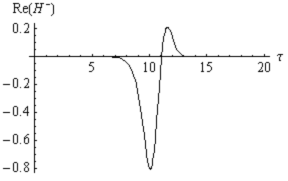
Figure 1: Numerical solution $\mathrm{Re}(H^{-})$ versus $\tau$ of system Eqs. (33), (34), (35), and (36) integrated in the complex plane. The initial conditions are $\mathrm{Re}(H^{+})=1-\mathrm{Re}(\psi^{+})=-10^{-4}\cos(\theta_{1})\cos(\theta_{2})$, $\mathrm{Re}(H^{-})=1-\mathrm{Re}(\psi^{-})=-10^{-4}\sin(\theta_{1})\cos(\theta_{2})$, $\mathrm{Im}(H^{+})=\mathrm{Im}(\psi^{+})=-10^{-4}\cos(\theta_{1})\sin(\theta_{2})$, $\mathrm{Im}(H^{-})=\mathrm{Im}(\psi^{-})=-10^{-4}\sin(\theta_{1})\sin(\theta_{2})$, $\theta_{1}=39\pi/200$, $\theta_{2}=\pi/2$.

We have numerically integrated system Eqs. (33), (34), (35), and (36); for an example see Fig. 1. These trajectories numerically define the self-similar profiles $\varphi^{\pm}(\cdot)$. We still have to check that the inverse Laplace transform formula (29) makes sense for these numerical solutions. It turns out that the functions $\varphi^{\pm}(\cdot)$ (considered as functions of the variable $\tau$, which is now considered to be complex) can be analytically extended to the regions $\mathrm{Re}(\tau)>L$, $\mathrm{Re}(\tau)<1/L$, $|\mathrm{Im}(\tau)|<\pi/2+\epsilon$ for some real $L$ sufficiently large and some real $\epsilon>0$ sufficiently small (see emv ). On the other hand, we have checked numerically that in fact there are no singularities for the functions $\varphi^{\pm}(\cdot)$ in the whole strip $|\mathrm{Im}(\tau)|<\pi/2+\epsilon$, $\mathrm{Re}(\tau)\in(-\infty,\infty)$. This implies that the functions $\varphi^{\pm}(\cdot)$ considered as functions of $\xi$ (considered also as a complex variable) are analytic in the half-plane $\mathrm{Re}(\xi)>0$ and therefore the function $\mathcal{G}^{\pm}(\cdot)$ can be obtained by means of the inversion formula for the Laplace transform (29). This numerically proves the existence of scaling solutions to coagulation Eq. (25) obeying the self-similar scaling (28).

IV Conclusions

To conclude, the emergent properties of physical systems are determined by the interactions among its fundamental constituents, but they could also be described and understood in terms of the interactions among the different subgroups conforming the whole. Consensus is the microscopic characteristic underlying macroscopic order in these systems, and it is reached or not depending on the interaction nature. In the specific case of the majority kernel considered in this paper, Eq. (19), the absence of consensus is due to the finely tuned balance between the transition probabilities of the kernel and the number of elements changing their state in each interaction. Kernel (19) can be easily generalized to models with the form:

$$\partial_{t}f^{\mp}(l,t)=\sum_{k+j=l}\left(\frac{k}{k+j}\right)^{\alpha}f^{\pm}(k,t)f^{\mp}(j,t)-\sum_{m}f^{\pm}(m,t)f^{\mp}(l,t),\qquad\alpha>0.$$ (39)

For this class of equations the finely tuned balance that takes place for $\alpha=1$ does not take place in general. An interesting mathematical question would be determining the range of values of $\alpha$ yielding consensus formation for these models. Notice that Eqs. (3) and (4) constitute an example of interaction kernel which does not preserve the balances among collisions, and thus leads to ordered long-range states, despite the seemingly weaker trend toward order implied by it when compared to the one in Eq. (39).

In the simple cases we have studied, consensus takes the form of one or several clusters travelling in the same direction. As two directions are possible, and the system is symmetric with respect to them, we note the similarity of this process with those systems with two symmetric absorbing states munoz ; lopez . It is clear that consensus is an absorbing state in our model, as collisions stop when consensus is reached. Complementarily, the active state is the one in which collisions still take place, which necessarily implies the existence of clusters travelling in both directions and the concomitant absence of consensus. We additionally note that for the dynamics given by the majority kernel described in the last section, consensus is not reached in the coagulation equation approximation. So this disordered state could be thought of as a long lived, deterministically stable, metastable state which will finally decay to one of the absorbing states due to the effects of fluctuations. We have of course not studied such effects in the present paper, so we simply mention the possible similarity of this process with the dynamics of certain systems characterized by the proximity to absorbing states. Establishing a rigorous connection is far beyond the scope of this work.

In the light of our results it seems possible that some self-organizing systems interact according to some rule which does not preserve the balance among the collisions or interactions at their different scales. Otherwise, as we have seen, if some moment is preserved then consensus is consequently not reached. As we have mentioned, these techniques may be applied or adapted to swarming and opinion formation systems. Our approach constitutes an idealized first approximation to these sorts of problems. More realistic approaches should deal with the effect of fluctuations and finite sizes and this way estimate how stochastic forces may influence ordering/disordering processes. Also, we have not taken into account the effect of saturation and fragmentation of clusters, which would keep the cluster masses finite. We have focused for simplicity on the short time behavior during which the initial growth of cluster masses could be described with the probabilistic rules we have considered herein. We leave for future work the implementation of these improvements.

References

- (1) I. D. Couzin, J. Krause, N. R. Franks, and S. A. Levin, Nature 433, 513 (2005).
- (2) F. Cucker, S. Smale, and D.X. Zhou, Found. Comput. Math. 4, 315 (2004).
- (3) C. Escudero, Phys. Rev. Lett. 101, 196102 (2008).
- (4) T. Lux and M. Marchesi, Nature 397, 498 (1999).
- (5) J. Seinfeld, Atmospheric Chemistry and Physics of Air Polution (New York, Wiley, 1986).
- (6) R. M. Ziff, J. Stat. Phys. 23, 241 (1980).
- (7) I. M. Lifshitz and V. V. Slyozov, J. Phys. Chem. Solids 19, 35 (1961).
- (8) M. Conti, B. Meerson, A. Peleg, and P. V. Sasorov, Phys. Rev. E 65, 046117 (2002).
- (9) J. Silk and S. D. White, Astrophys. J. 223, L59 (1978).
- (10) H. S. Niwa, J. Theor. Biol. 195, 351 (1998).
- (11) M. R. D’Orsogna, Y. L. Chuang, A. L. Bertozzi, and L. S. Chayes, Phys. Rev. Lett. 96, 104302 (2006).
- (12) M. Bodnar and J. J. L. Velázquez, J. Diff. Eqs. 222, 341 (2006).
- (13) M. R. D’Orsogna, V. Panferov, and J. A. Carrillo, Kinetic and Related Models 2, 363 (2009).
- (14) A. Czirók, A.-L. Barabási, and T. Vicsek, Phys. Rev. Lett. 82, 209 (1999).
- (15) R. Toral and C. J. Tessone, Commun. Comput. Phys. 2, 177 (2007).
- (16) C. Castellano, S. Fortunato, and V. Loreto, Rev. Mod. Phys. 81, 591 (2009).
- (17) P. Clifford and A. Sudbury, Biometrika 60, 581 (1973).
- (18) R. Holley and T. M. Liggett, Ann. Prob. 3, 643 (1975).
- (19) T. M. Liggett, Interacing Particle Systems (Springer-Verlag, New York, 1985).
- (20) E. Hernández-García and C. López, Phys. Rev. E 70, 016216 (2004).
- (21) C. Huepe and M. Aldana, Phys. Rev. Lett. 92, 168701 (2004).
- (22) F. Peruani, A. Deutsch, and M. Bär, Phys. Rev. E 74, 030904(R) (2006).
- (23) M. Pineda, R. Toral, and E. Hernández-García, J. Stat. Mech. P08001 (2009).
- (24) J. Buhl, D. J. T. Sumpter, I. D. Couzin, J. J. Hale, E. Despland, E. R. Miller, and S. J. Simpson, Science 312, 1402 (2006).
- (25) C. A. Yates, R. Erban, C. Escudero, I. D. Couzin, J. Buhl, I. G. Kevrekidis, P. K. Maini, and D. J. T. Sumpter, Proc. Natl. Acad. Sci. USA 106, 5464 (2009).
- (26) J. B. McLeod, Proc. London Math. Soc. 14, 445 (1964).
- (27) M. Kreer and O. Penrose, J. Stat. Phys. 75, 389 (1994).
- (28) G. Menon and R. L. Pego, Commun. Pure Appl. Math. 57, 1197 (2004).
- (29) C. Escudero, F. Macià, and J. J. L. Velázquez, preprint.
- (30) G. Arfken, Mathematical Methods for Physicists, 3rd ed. (Academic Press, Orlando, 1985).
- (31) J. M. Ball and J. Carr, J. Stat. Phys. 61, 203 (1990).
- (32) O. Al Hammal, H. Chaté, I. Dornic, and M. A. Muñoz, Phys. Rev. Lett. 94, 230601 (2005).
- (33) F. Vázquez and C. López, Phys. Rev. E 78,061127 (2008).