The Relation Between Halo Shape, Velocity Dispersion and Formation Time

Abstract

We use dark matter haloes identified in the MareNostrum Universe and galaxy groups identified in the Sloan Data Release 7 galaxy catalogue, to study the relation between halo shape and halo dynamics, parametrizing out the mass of the systems. A strong shape-dynamics, independent of mass, correlation is present in the simulation data, which we find it to be due to different halo formation times. Early formation time haloes are, at the present epoch, more spherical and have higher velocity dispersions than late forming-time haloes. The halo shape-dynamics correlation, albeit weaker, survives the projection in 2D (ie., among projected shape and 1-D velocity dispersion). A similar shape-dynamics correlation, independent of mass, is also found in the SDSS DR7 groups of galaxies and in order to investigate its cause we have tested and used, as a proxy of the group formation time, a concentration parameter. We have found, as in the case of the simulated haloes, that less concentrated groups, corresponding to late formation times, have lower velocity dispersions and higher elongations than groups with higher values of concentration, corresponding to early formation times.

Morphology & Dynamics of Group Size Haloes

1 INTRODUCTION

According to the hierarchical model of structure formation, groups and clusters of galaxies, embedded in dark matter haloes, emerge from Gaussian primordial density fluctuations and grow by accreting smaller structures, formed earlier, along anisotropic directions. Such structures constitute therefore an important step in the hierarchy of cosmic structure formation and are extremely important in deciphering the processes of galaxy and structure formation. It should thus be expected that recently formed structures are highly elongated, reflecting exactly the anisotropic distribution of the large-scale structure from which they have accreted their mass, and dynamically young. Therefore the determination of the dynamical state of groups and clusters of galaxies and its evolution, which could be affected by a multitude of factors - like environment, formation time, etc - is a fundamental step in investigating the hierarchical galaxy formation theories.

Both analytical calculations and N-body simulations have consistently shown that the virialization process will tend to sphericalize the initial anisotropic distribution of matter, and therefore the shape of haloes is an indication of their evolutionary stage. Furthermore, the halo shape, size, and velocity dispersion (among others) are important factors in determining halo member orbits and interaction rates, which are instrumental in understanding galaxy formation and evolution processes (eg., Jing & Suto 2002; Kasun & Evrard 2005; Avila-Reese et al. 2005; Bailin & Steinmetz 2005; Allgood et al. 2006; Bett et al. 2007; Ragone-Figueroa & Plionis 2007; Macció, Dutton, van den Bosch 2008 and references therein). It has been found that dark-matter haloes are triaxial but with a strongly preferred prolatness (eg., Plionis, Basilakos & Ragone-Figueroa 2006; Gottlöber & Yepes 2007 and references therein) and that there is also a correlation between the orientation of their major axes and the surrounding structures. Such alignment effects, among relatively massive haloes, have been found to be particularly strong (eg., Faltenbacher et al. 2002; Kasun & Evrard 2005; Hopkins, Bachall & Bode 2005; Ragone-Figueroa & Plionis 2007; Faltenbacher et al. 2008 and references therein). There are indications that the mentioned correlation might arise, or strengthen, from re-arrangements of the orientation of the halo axes in the direction from which the last major merger event occurred [van]. Hence, the shape of dark matter haloes might well be correlated with the large scale structure, providing clues to the fashion in which mass is aggregated (eg., Basilakos et al. 2006). The imprints of this accretion can be observed in the substructure features present in a halo, which have been found to correlate with the halo shape (Ragone-Figueroa & Plionis 2007). Haloes with higher levels of substructure, or equivalently dynamically young haloes, are preferentially more elongated. The subsequent evolution should induce a change in the shape of haloes, leading to more spherical configurations, increasing their velocity dispersions as well.

According to this last statement, Faltenbacher & Mathews (2007) have found, in agreement with the Jeans equation, that the velocity dispersion of sub-haloes increases with the host halo concentration. Given that halo concentration and formation time are also correlated (Bullock et al. 2001; Wechsler et al. 2002), this result implies that older haloes should have higher sub-halo velocity dispersions. Once a halo is virialized, the dynamical mass can be computed from their velocity dispersion and virial radius (eg., Binney & Tremaine 1987). Nevertheless, if virialization has not yet been achieved, the above mentioned effect and its possible dependence to the local halo environment should be taken into account. In addition, there is also evidence for the sphericalization of DM haloes with time (e.g. Allgood et al. 2006). This behavior can be well studied using haloes in numerical simulations, where their 3D shape and velocity dispersion can be calculated accurately.

These issues motivated us to study the relation between the DM halo velocity dispersion and shape, in narrow halo mass ranges, in order to exclude the possible halo-mass dependent effects. We also investigate how this correlation is transformed when computing projected shapes and velocity dispersion along the line-of-sight, in order to be able to compare with observational data, like the SDSS galaxy groups.

The plan of the paper is the following. In section 2 we describe the MareNostrum numerical simulation and the SDSS observational data together with the identification procedure of the corresponding systems and their properties. In section 3 we study the halo shape-dynamics relation in the simulation. In section 4 we seek for a formation-age proxy which can be computed in a realistic group catalog. We continue in section 5 by presenting the shape-dynamics correlation results for the observed SDSS groups of galaxies. Finally, section 6 contains our conclusions.

2 THE HALO & GROUP DATA

2.1 The MareNostrum Simulation

This non-radiative SPH simulation, dubbed The MareNostrum Universe (see Gottlöber & Yepes 2007) and covering a volume of $(500\;h^{-1}{\rm Mpc})^{3}$, was performed in 2005 with the parallel TREEPM+SPH Gadget2 code (Springel 2005). The resolution of the simulation is such that the gas and the DM components are resolved by $2\times 1024^{3}$ particles. The initial conditions at redshift $z=40$ were calculated assuming a spatially flat concordance cosmological model with the following parameters: the total matter density $\Omega_{m}=0.3$, the baryon density $\Omega_{b}=0.045$, the cosmological constant $\Omega_{\Lambda}=0.7$, the Hubble parameter $h=0.7$, the slope of the initial power spectrum $n=1$ and the normalization $\sigma_{8}=0.9$. This resulted in a mass of $8.3\times 10^{9}h^{-1}{{\cal M}_{\odot}}$ for the DM particles and $1.5\times 10^{9}h^{-1}{{\cal M}_{\odot}}$ for the gas particles. The simulation followed the nonlinear evolution of structures in gas and dark matter from $z=40$ to the present epoch. Dissipative or radiative processes or star formation were not included. The spatial force resolution was set to an equivalent Plummer gravitational softening of $15\;h^{-1}$ comoving kpc. The SPH smoothing length was set to the distance to the 40^th nearest neighbor of each SPH particle.

After the release of the 3-year WMAP data the original simulation has been repeated with lower resolution assuming the predicted low WMAP3 normalization ($\sigma_{8}=0.75$) as well as with a higher normalization of $\sigma_{8}=0.8$, which is better in agreement with the 5-year WMAP data. Yepes at al. (2007) argue that the low normalization cosmological model inferred from the 3 year WMAP data results is barely compatible with the present epoch X-ray cluster abundances. All these simulations have been performed within the MareNostrum Cosmology project at the Barcelona Supercomputer Center.

2.1.1 Halo identification, shape & formation time

In order to find all structures and substructures within the distribution of 2 billion particles and to determine their properties we have used a hierarchical friends-of-friends algorithm (Klypin et al. 1999, Gottlöber et al. 2006b). At all redshifts we have used a basic linking length of 0.17 of the mean inter-particle separation to extract the FOF clusters, which corresponds to an overdensity of $\sim$330 of the mean density. Shorter linking lengths have been used to study substructures. The FOF analysis has been performed independently over DM and gas particles. Using a linking length of 0.17 at redshift $z=0$ we have identified more than 2 million objects with more than 20 DM particles which closely follow a Sheth-Tormen mass function (Gottlöber et al. 2006a).

Using the FOF method one extracts rather complex objects from the simulation which are characterized by an iso-density surface given by the linking length. In first approximation these objects can be characterized by triaxial ellipsoids. The shape and orientation of the ellipsoids can be directly calculated as eigenvectors of the inertia tensor of the given object. Then the shape is characterized by the ratios between the lengths of the three main axes ($a>b>c$). Gottlöber & Yepes 2007 have studied the shape of the galaxy clusters in the The MareNostrum Universe and found that both the gas and dark matter components tend to be prolate although the gas is much more spherically distributed. Here we study the shape of the more massive dark matter component of the FOF objects which reflects the shape of the potential in which the galaxies move.

Finally, in our present work we will extensively use the notion of halo formation time ($z_{\rm form}$), which is usually defined as the redshift at which the halo accretes half of its final ($z=0$) mass. By selecting haloes in the lower and upper quartiles of the formation time distribution, we define what we will call the late formation time (LFT) and early formation time (EFT) halo populations, respectively. We also divide the haloes in four mass ranges, namely $1.0-1.3$, $2.0-2.5$, $3.2-4.0$ and $6.3-7.9\times 10^{13}h^{-1}{{\cal M}_{\odot}}$, since we wish to cancel the dependence of any halo-based parameter on its mass.

Figure 1 shows the distribution of formation times for the four subsamples of haloes as defined previously. The vertical dashed lines denote the location of the first and fourth quartile of the distribution.

Figure 1: Different panels correspond to the formation time distribution of haloes in a different range of mass, namely $1.0-1.3$, $2.0-2.5$, $3.2-4.0$ and $6.3-7.9\times 10^{13}h^{-1}{{\cal M}_{\odot}}$, from left to right and top to bottom. Vertical dashed lines denote the first and fourth quartile of the distribution.

2.2 SDSS DR7 Galaxy Groups

Figure 2: Fractional distribution of virial radii (left panel) and masses (right panel) of groups in a volume limited sample (with 10 or more members) extracted from the SDSS DR7 corresponding to $0.06<z<z_{\rm lim}=0.10$ (dashed histogram), compared to that corresponding to the total sample of groups (with 3 or more members) up to $z=0.10$ (empty histogram).

In recent years a considerable effort has been invested in identifying, using a multitude of methods, groups and clusters of galaxies in redshift surveys (e.g. Huchra & Geller 1982; Tully 1987; Nolthenius & White 1987; Ramella et al. 2002; Merchán & Zandivarez 2002, 2005; Gal et al. 2003; Gerke et al. 2004; Lee et al. 2004; Lopes et al. 2004; Eke et al. 2004; Tago et al. 2006, 2008; Berlind et al. 2006; Crook et al. 2007; Yang et al. 2008; Sharma & Johnston 2009; Finoguenov et al. 2009).

In this work we identify groups of galaxies in the SDSS DR7 spectroscopic galaxy sample, which comprises of more than 900000 galaxies, within an area of approximately 9000 square degrees, and with a limiting r-band magnitude of $m_{\rm lim}=17.77$. The group finding algorithm is based on the procedure detailed in Merchán & Zandivarez (2005) and consists in using the friends-of-friends algorithm, similar to that developed by Huchra & Geller (1982). The algorithm links galaxies ($i$ and $j$) which satisfy $D_{ij}\leq D_{0}R(z)$ and $V_{ij}\leq V_{0}R(z)$, where $D_{ij}$ is their projected distance and $V_{ij}$ is their line-of-sight velocity difference. The scaling factor $R(z)$ is introduced in order to take into account the decrement of the galaxy number density due to the apparent magnitude limit cutoff. We have adopted a transverse linking length $D_{0}$ corresponding to an overdensity of $\delta\rho/\rho=80$ and a line-of-sight linking length of $V_{0}=200\rm{km~{}s^{-1}}$.

In order to avoid significant discreetness effects in the group shape and dynamics determination, we limit our catalogue to those groups with more than ten members ($n_{m}\geq 10$). To further avoid artificial redshift-dependent effects (eg., Frederic 1995; Plionis et al. 2004; Plionis et al. 2006) and to build a roughly volume limited sample, we select those groups with $0.06<z<0.1$ and $M_{10}<M_{\rm lim}$, where $M_{10}$ is the absolute magnitude of the $10^{th}$ brighter galaxy and $M_{\rm lim}(=-19.53)$ is the absolute magnitude of a galaxy with apparent magnitude $m=m_{\rm lim}$ at $z=0.1$. The resulting sample, within the previously mentioned $z$-range, comprises 760 groups with at least ten member galaxies.

For these groups, we compute their virial radius, line of sight velocity dispersion ($\sigma_{z}$) and virial mass ($\cal M$), following Merchán & Zandivarez (2005). In Figure 2 we present the distribution of virial masses and radii of the resulting groups, comparing with those of the whole ($n_{m}\geq 3$ and $z<0.1$) parent group sample. It is evident that we are preferentially selecting the richest systems, which is the price we have to pay for producing a volume limited subsample.

2.2.1 Group Projected Shape

The group elongation is determined by diagonalizing the ”inertia” tensor, which we construct weighting each galaxy $n$ by its luminosity $L_{n}$. This is done in order to weight more the galaxies that dominate in shaping the group gravitational potential:

$$I_{ij}=\sum_{n=1}^{10}L_{n}~{}x_{i,n}~{}x_{j,n},$$ (1)

where $x_{i,n}$ is the $i^{th}$ component of the position vector of the $n^{th}$ galaxy relative to the group center of mass. Diagonalizing the $I_{ij}$ tensor we obtain two eigenvalues which are related to the square root of the minor and major axes, $b$ and $a$ respectively, which define the halo axial ratio: $q=b/a$.

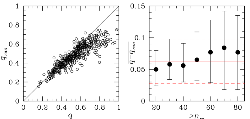
Figure 3: Left panel: The $q-q_{ran}$ scatter plot for groups within the volume limited sample and with at least 20 member galaxies. Right panel: The median value of $q-q_{ran}$ as a function of minimum number of group galaxy members. Errorbar correspond to the 33% and 67% quantiles. The solid line corresponds to the value $q-q_{ran}=0.063$ and the dashed lines to the $\pm 0.035$ range.

Furthermore, as it is well documented, there exists a dependence of the group halo apparent elongation on the member-number resolution of the system (eg., Paz et al., 2006; Plionis, Basilakos & Ragone-Figueroa, 2006). According to this effect, a given system will appear artificially more elongated (smaller $q=b/a$ ratio) when sampled by a lower number of members. This effect however is large for groups with less than ten members (see fig.3 in Plionis et al. 2006) and therefore it should not affect significantly our group sample, which by construction has $n_{m}\geq 10$. In any case and to overcome any residual effect which could be introduced due to the variable resolution of the different groups, we sample each group having $n_{m}>10$ by selecting randomly only ten galaxies, which is the number resolution of the lowest $n_{m}$ galaxy groups in our sample. Finally, the adopted value of the projected shape, $q_{ran}$, is the result of computing the mean of 10 realizations of the random galaxy selection procedure. By this procedure we degrade the accuracy of the shape parameter of groups with $n_{m}>10$, but we gain resolution consistency over all our group sample. To get an idea of the uncertainty introduced by our procedure, we present in the left panel of Figure 3 the $q$ vs. $q_{ran}$ correlation. As expected, the $q_{ran}$ values are systematically lower than their counterparts, $q$, computed using all member galaxies, while the deviation increases for the intrinsically more spherical systems. Since in this plot we show together all groups with $n_{m}\geq 20$, in the right panel of Fig.3 we plot the median value of $q-q_{ran}$ as a function of minimum number of group member galaxies. It can be seen than there is, as expected, a tendency of $q-q_{ran}$ to slowly increase with $n_{m}$ but, within the errors, we can quote an overall median value of: $\overline{q-q_{ran}}\simeq 0.063\pm 0.035$, independent of $n_{m}$.

Figure 4: Each panel corresponds to haloes in the four different ranges of mass, increasing in mass for the top left, to top right, then bottom left and bottom right panels, respectively. The left box of each panel shows the isodensity contours of $c/a$ vs $\sigma_{v}$ for all haloes in the corresponding range of mass. The right box of each panel shows the corresponding isodensity contours but only of the 25% and 75% quantiles of the formation time distribution, which correspond to the EFT (solid line) and LFT (dotted line) families of haloes.

3 THE HALO SHAPE-DYNAMICS RELATION

In this section we investigate the relation between morphology and dynamical status of DM haloes.

As it is well known halo properties can have a strong dependence on halo mass. Especially, the velocity dispersion of virialized or nearly virialized haloes are related to the halo mass through the virial theorem: $M\propto\sigma^{2}$. Therefore, in order to search for an intrinsic dependence of the velocity dispersion on shape, it is imperative to suppress their possible dependence to mass, due to the virialization expectation. To this end we have studied the shape-$\sigma_{v}$ correlation, in the four mass ranges defined in section (2.1.2), both in 3D-space and in projected 2D-space (using 1D velocities and projected halo shapes).

3.1 3D Halo $c/a-\sigma_{v}$ Correlation

Figure 4 shows the isodensity contours of the shape-$\sigma_{v}$ scatter plot, at redshift $z=0$, for some of the selected mass bins (left boxes of each panel). As it can be seen, there exists a clear correlation between halo sphericity and halo velocity dispersion, according to which more spherical haloes have higher velocity dispersions. Even though we have been cautious in selecting small mass ranges, the observed behavior could, in principle, be attributed to the halo mass variation within each mass-bin. For this to be true the more massive systems within each bin - which should also be the higher velocity dispersion ones - should have the highest values of the $c/a$ ratio. However, it is well established that more massive systems tend to be less spherical (e.g. Allgood et al. 2006). Therefore, the observed correlation cannot be attributed to a possible residual dependence on halo-mass. A rather interesting possibility is related to the fact that haloes, of any given mass and at any given cosmic epoch, could have a different formation time as well as a different evolutionary history.

Under this hypothesis, and in order to further investigate the dependence of shape-$\sigma_{v}$ correlation on the halo formation time ($z_{\rm form}$), we plot separately the EFT and LFT $c/a-\sigma_{v}$ correlations in the right boxes of each panel of Figure 4. It is evident that two populations occupy clearly delineated regions in the $c/a-\sigma_{v}$ plane, with the EFT haloes (solid line) typically having higher velocity dispersions and higher sphericities than the LFT haloes (dotted line). It can be also observed that the LFT contours cover a wider range of $\sigma_{v}$ values than the corresponding EFT ones, but they do not reach the highest EFT sphericities. Finally, it is interesting to also note that there is a shift of the peak of the LFT contours towards lower $c/a$’s and $\sigma_{v}$’s between the lower mass (upper panels) and the higher mass LFT halos (lower panels). This could be attributed to a fraction of the most massive LFT systems being relatively more dynamically young and in the phase of primary mass aggregation. We will return to this issue later on.

As it is obvious from Figure 4, the same overall trend, between the LFT and EFT halos, is present in all mass bins. It would be ideal then, in order to enhance the statistical validity of our results, to combine the information contained in the different mass ranges in a unique, independent of halo mass, analysis. This would also facilitate the corresponding study of the observational data, since the available number of SDSS groups is significantly smaller than that of the simulated haloes and thus we cannot afford to divide them in many mass subsamples.

Since the parameters under study ($\sigma_{v}$, $c/a$ and $z_{\rm form}$) depend on halo mass, we have devised a normalization procedure that imposes the mass independence of the results and combines in a unique relation the halo velocity dispersion and shape of the whole sample. In detail we derive normalization functions of the different parameters by computing analytic fits of the relation between the corresponding parameter ($P$) and the halo mass (${\cal M}$). Then for a given halo mass we normalize each of the three parameter under study to the value expected from the analytic fit ($\overline{P}({\cal M})$).

Since it is no longer necessary to split haloes in narrow mass bins we can use the entire main sample of haloes to plot in Figure 5 the normalized, independent of mass, shape-dynamics correlation. It is evident that the EFT and LFT behavior, seen in Figure 4, is reproduced for the whole halo sample and we have further verified that these results are indeed independent of halo mass. In the inset of Figure 5 we show that the corresponding distribution of masses of the EFT (solid line) and LFT (dashed line) populations are statistically equivalent and therefore there is no residual mass-dependent effect affecting the correlation shown in the main panel.

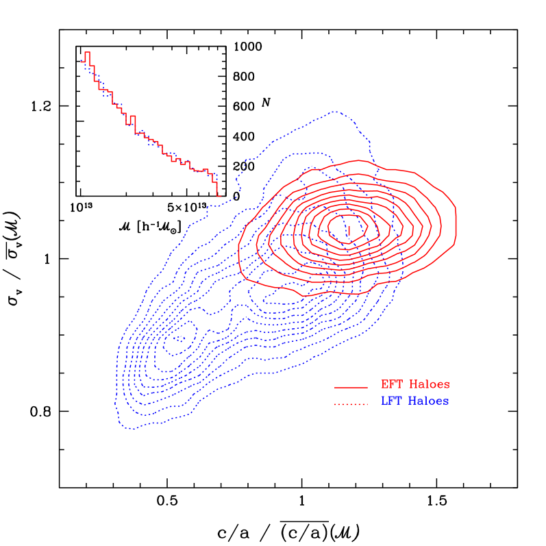
Figure 5: Normalized $c/a$-$\sigma_{v}$ relation for EFT (solid line) and LFT (dashed line) populations. All masses are considered. The formation time used to divide EFT and LFT is also normalized to the expected value for a given mass (see text). Inset panel: Distribution of masses of the EFT (solid line) and LFT (dashed line) populations demonstrating that no mass effect is present in the result obtained in the main panel.

Table 1: The Spearman coefficient (SC) for the velocity dispersion-shape correlation for haloes in four mass bins. In all cases (3D and 2D) the correlations of the EFT haloes is significantly lower than that of the LFT haloes.

Sample	Mass [$\times 10^{13}{\cal M}_{\odot}h^{-1}$]
	1.0-1.3	2.0-2.5	3.2-4.0	6.3-7.9
3D All	0.37	0.42	0.44	0.48
3D LFT	0.45	0.55	0.60	0.72
3D EFT	0.11	0.16	0.21	0.22
2D All	0.27	0.31	0.33	0.34
2D LFT	0.31	0.38	0.42	0.47
2D EFT	0.11	0.12	0.15	0.18

Our main results, as extracted from Figures 4 and 5, can be tabulate as follows: (a) The LFT haloes show a significantly stronger $c/a-\sigma_{v}$ correlation than the EFT haloes, while they also span a wider range of values, (b) The LFT $\sigma_{v}$ values are, in some cases, even higher than those of the EFT (”virialized”) halo population, (c) A bimodal pattern is present in the $\sigma_{v}-c/a$ plane (Figure 5) with two local maxima, one of which is situated at the low velocity dispersion and low $c/a$ values, which as we have discussed earlier and deduced from Figure 4, it is caused by the more massive haloes. Below we attempt to interpret individually each of the above results:

(a) Different $\sigma_{v}-c/a$ correlation strength of the EFT and LFT haloes: The apparent lack of a strong correlation of the EFT halo population should be attributed to the fact that EFT haloes had plenty of time to virialize and that the virialization process erases the intrinsic shape-$\sigma_{v}$ correlation. To quantify the strength of the shape-$\sigma_{v}$ correlation we estimate the Spearman correlation coefficient as a function of halo mass (Table 1). Clearly the observed strong and significant correlation of the whole halo population should be attributed to the LFT haloes, since (as we already discussed) the EFT haloes show very weak shape-$\sigma_{v}$ correlations.

So far, the results obtained suggest that the intrinsic halo shape-$\sigma_{v}$ correlation, within each small mass range, is the consequence of the coexistence of haloes of different formation times, going through different evolutionary phases. Dark matter haloes, in the initial stages of formation and before virialization is complete, have typically a smaller velocity dispersion and a more elongated shape. Once virial equilibrium is reached these quantities stabilize and, since this equilibrium configuration is more likely to be achieved by the early formation time haloes, the EFT family shows only a weak such shape-$\sigma_{v}$ correlation.

We attempt to investigate in more detail the evolution paradigm, as the cause of the $\sigma_{v}-c/a$ correlation, by dividing the halo formation-time distribution in eight quantilies. We then compute the median values of $\sigma_{v}/(\overline{\sigma}({\cal M}))$ and $c/a/(\overline{(c/a)}({\cal M}))$ within each $z_{\rm form}$ quantile and plot them in Figure 6. In concordance with Figure 5, we consistently find a clear trend indicating that the earlier the halo is formed, the higher its $\sigma_{v}$ and $c/a$ ratio, as expected from the fact that older haloes have more time to evolve and virialize. Evidently, a halo evolutionary sequence appears, with dynamically young haloes situated at the lower-left of the $c/a-\sigma_{v}$ plane and as they evolve, they move towards higher $\sigma_{v}$ and $c/a$ values, where the virialized haloes are located.

Figure 6: Normalized $c/a-\sigma_{v}$ trend corresponding to the entire sample of haloes. Each point corresponds to the median $c/a/(\overline{(c/a)}({\cal M}))$ and $\sigma_{v}/(\overline{\sigma_{v}}({\cal M}))$ values computed for haloes with $z_{\rm form}$ within different octiles of formation time. Error bars mark the 10% percentile of the corresponding distribution.

Note, however, that in Figure 6 the dynamically youngest haloes (1st octile of formation time) show a behaviour that deviates from the overall trend, being characterized by a lower normalized $c/a$ value. This outlier has a relatively larger uncertainty with respect to the other octiles, and a possible cause of this behaviour is presented in (c).

(b) LFT haloes with $\sigma_{v}$ values even larger than those of EFT haloes: In an attempt to explain what is the cause of the rather unexpected behavior of some LFT haloes, i.e., those having relatively high sphericity and in the same time a velocity dispersion which is as large or even larger than what expected from the “virialized” EFT haloes, we suggest two mechanisms:

• Since LFT haloes are prone to have had a recent merger and since it is expected that dynamical interactions and merging processes increase the velocity dispersion of the involved systems some merging or highly interacting haloes could be undergoing a transient geometrical configuration of high sphericity (resulting when the in-falling substructures are near the perigee), while temporarily achieving a velocity dispersion which could be even larger than their virial value (Faltenbacher et al. 2006). We have verified that indeed this is the case for some of the LFT haloes.

• Part of the high velocity dispersion and quasi-spherical LFT haloes could be due to truly virialized LFT haloes by a somewhat rapid virialization process depending on their particular formation history and/or environment.

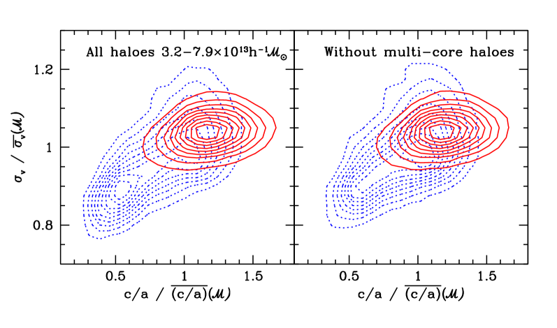
Figure 7: Same as Figure 5 but only considering haloes with masses between $3.2$ and $7.9\times 10^{13}h^{-1}{{\cal M}_{\odot}}$. In the left panel the entire sample is used whereas in the right panel all double-core haloes have been excluded.

(c) The two maxima in the LFT $\sigma_{v}-c/a$ correlation plane: As we have discussed earlier, the lower $\sigma_{v}-c/a$ maximum seen in Figure 5 is caused by the most massive haloes (ie., those with ${\cal M}\raise-2.0pt\hbox{\hbox to0.0pt{\hbox{$\sim$}\hss}\raise 5.0pt\hbox{$>$}\ }3.2\times 10^{13}\;h^{-1}\;{\cal M}_{\odot}$) and could be attributed to a fraction of the most massive LFT systems being relatively dynamically younger and in the phase of merging, where the FOF algorithm could join a merging pair into a single FOF halo.

In order to verify our suspision we have selected haloes with masses between $3.2-7.9h^{-1}{{\cal M}_{\odot}}$ (including the two most massive ranges presented in Figure 4, where the bimodal pattern was evident for the LFT haloes) and investigated in which manner the described trend would be affected if double (or multiple)-core halos (or otherwise dumbbell shaped haloes) were excluded. Double-core haloes were identified as those haloes that are split in two or more subhaloes of at least 1000 particles, within a relative distance of 2$r_{\rm sph}$ ($r_{\rm sph}$ is the diameter of a sphere which has the same volume as the considered halo), when a re-identification with a shorter linking length (0.135 of the mean interparicle separation) is performed. Therefore, they are major pre-merger systems which the FOF joins into a single system and which other halo-finders would have probably singled out each component as an individual halo. In the left panel of Figure 7 we show the $c/a-\sigma_{v}$ correlation when all haloes in the mentioned mass range are considered, whereas in the right panel double-core haloes are excluded. It is evident that the secondary maximum at low $\sigma_{v}$ and $c/a$, is caused by the double-core haloes, which are those that are in an active major merger process, and thus an integral part of the “dynamically young” family of haloes. Note, that although the $c/a-\sigma_{v}$ LFT correlation is weakend when excluding the double (multiple)-core haloes, it is still clearly present.

Returning to the issue of the “outlier” seen in Figure 6, we have verified that the cause of the significantly smaller normalized $\langle c/a\rangle$ value of the first formation time octile is the significantly larger number of double (multiple)-core haloes found in this octile with respect to the other octiles. For example, for the case of the most massive haloes (ie., those investigated in Figure 7) we find that $\sim 22\%$ of the haloes in the first octile are double (multiple)-core haloes, while this number drops to $4.8\%$ and $2.6\%$ in the second and third octile respectively, and to even smaller values thereafter.

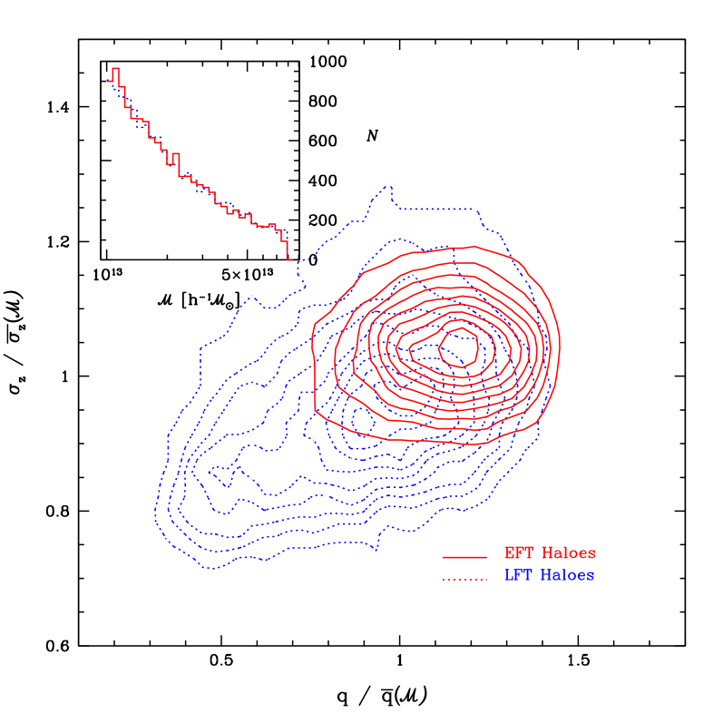
Figure 8: As in Fig.5 but using projected halo shapes and 1D velocity dispersions.

3.2 2D Halo $q-\sigma_{z}$ Correlation

Here we present the corresponding analysis of the previous subsection, but using the projected halo axial-ratio ($q=b/a$ obtained from the projected particle distribution) and the one-dimensional velocity dispersion. This is done in order to see how the previous (3D) results are translated into theoretical expectations that can be compared with the results based on observational group samples.

Figure 8 is the 2D analogue of Figure 5 and we can clearly see that qualitatively the correlation revealed in Figure 5, albeit weaker, is repeated in Figure 8. Details and significances may differ (see Table 1 for different mass ranges), however, the main result is that we expect to see (in realistic group samples) hints of an independent of mass correlation of the projected halo axial-ratio with its line-of-sight velocity dispersion.

4 A Formation Time Proxy

The aim of this section is to provide a formation-age proxy, tested with simulated haloes, but that it can also be computed in realistic groups of galaxy samples, where the adopted definition of $z_{\rm form}$ is not usable. This is done in order to test the morphology-dynamics-formation time correlation (which was found to be present in simulated haloes) in groups extracted from the SDSS DR7.

We propose as a halo formation-age proxy ($\Delta_{\rm subh}$), the fraction of mass that is associated to the most massive substructure (subhalo), when a further re-identification is performed with a linking length which equals half the original one ($0.17/2$ of the mean inter-particle separation). This proposed parameter can be interpreted as a concentration indicator since it accounts for the distribution of mass at two different overdensities (given by the used linking lengths).

The number of particles of a halo in each overdensity level is defined as $n_{\rm high}$ and $n_{\rm low}$ for the higher and lower overdensities, respectively. Then the concentration parameter is given by:

$$\Delta_{\rm subh}=\frac{n_{\rm high}}{n_{\rm low}}\;.$$ (2)

The parameter $\Delta_{\rm subh}$ takes values within the range $\Delta_{\rm subh}\in[0,1]$, with a value near 1 indicating a high concentration and a value near 0 indicating the opposite. We show in Figure 9 the relation between $\Delta_{\rm subh}$ and halo formation redshift for the different ranges of mass labeled in the plot. It is evident that the oldest haloes have the highest levels of concentration, whereas the youngest ones extend to lower values of $\Delta_{\rm subh}$.

Figure 9: The $\Delta_{\rm subh}$ parameter as a function of formation time computed for dark matter haloes in four ranges of halo mass.

Since the above analysis clearly demonstrates that the proposed parameter can be used as an age indicator, we continue with the computation of the concentration parameter corresponding to galaxy groups in the observational data, $\Delta_{\rm sub}$. To this end we perform a second friends-of-friends identification, but this time using an overdensity of $\delta\rho/\rho=300$. This procedure allows us to extract a denser subgroup, of a given system, with respect to the original $\delta\rho/\rho=80$ sample. Then $\Delta_{\rm sub}$ is given by the ratio between the number of members of the denser subgroup to the number of members of its parent ($\delta\rho/\rho=80$) group. Utilizing this formation-age proxy, we examine the SDSS-DR7 group shape-dynamics-formation time relation in the next section.

5 The Shape-Velocity dispersion Relation of SDSS DR7 Groups

Many studies have attempted to determine the morphology and dynamical status of groups of galaxies (eg. Hickson et al. 1984; Malykh & Orlov 1986; Orlov, Petrova, Tarantaev 2001; Kelm & Focardi 2004, Plionis, Basilakos & Tovmassian 2004; Plionis, Basilakos, & Ragone-Figueroa 2006; Da Rocha, Ziegler, & Mendes de Oliveira 2007; Coziol & Plauchi-Frayn 2007; Wang et al. 2008; Hou et al. 2009) and have found that their morphology corresponds to that of mostly prolate-like triaxial ellipsoids (see however Robotham, Phillips & de Propris 2007), while there also appears to be a correlation between velocity dispersion and projected group shape (eg. Tovmassian & Plionis 2009) similar to what we found in the previous section.

Here we analyse our “volume-limited” group catalogue based on the SDSS DR7 galaxy survey, which was described in section 2.

As we have concluded in section 3.2, the shape-$\sigma$ correlation for dark matter haloes, extracted from the simulation, survives in projection but it is significantly weakened when the projected shape ($q$) and the one dimensional velocity dispersion are used. Further scatter should be expected in a more realistic situation in which the projected shape of SDSS groups are computed using only ten members ($q_{ran}$). Indeed, as it was shown in section 2.2, the typical error, expected when only ten members are considered, in the estimation of the projected shape is non-negligible. Such issues may act as to hide the morphology-dynamics correlation of observed groups of galaxies, and thus even a weak such correlation should be considered as a hint of a true underlying effect. We show in Figure 10 the least square best fit line of the $q_{ran}$ vs. $\sigma_{z}/\bar{\sigma_{z}}({\cal M})$ scatter plot (of the entire sample of galaxy groups) where the observed trend is in full agreement with Figure 8.

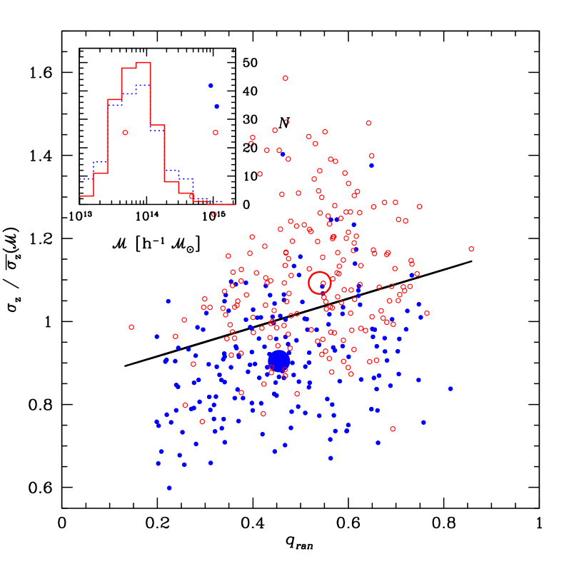
Figure 10: $q_{ran}$ vs. normalized $\sigma_{z}$ relation for groups in the SDSS DR7. Filled (low concentration) and empty (high concentration) dots stand for groups in the first and last quartile of the normalized $\Delta_{\rm sub}$ distribution, respectively. The large circles correspond to the median values. Solid line shows the least square fit using all the groups, irrespective of their $\Delta_{\rm sub}$ value. The inside box shows the mass distributions for groups in the cuartiles of low and high concentration (dotted and solid lines respectivelly).

We now attempt to investigate whether the observed $q_{ran}$ vs. $\sigma_{z}$ correlation, in Figure 10, is due to the coexistence of groups of different formation times, as was indeed shown to be the case in the dark matter halo analysis. As shown in section 3.2 (see also Figure 8), using projected shapes and one dimensional velocity dispersions does not completely mask the systematic behaviour observed for haloes of different formation times. However, taking into account the unfeasibility of determining the formation time of the observed galaxy groups, we use as a proxy of the group dynamical age its concentration parameter, $\Delta_{\rm sub}$. This parameter has indeed been shown (for the case of DM haloes) to correlate with halo formation time (see section 4).

In Figure 10 we separately plot groups of the first and last quartile of the $\Delta_{\rm sub}$ parameter distribution (as was done for formation time in section 3.1). Filled and empty circles represent galaxy groups with low and high concentration (corresponding to groups in the first and last quartiles of the $\Delta_{\rm sub}$ distribution), respectively. The tendency for high concentrated groups (open circles) to have systematically higher velocity dispersions and $q$ values is quite evident. We also plot their corresponding median values as large filled and empty circles, from which it can be seen that indeed there is a separation of the two families (based on $\Delta_{\rm sub}$), in both $q_{ran}$ and $\sigma_{z}$ axes. We have again verified that the observed behaviour is not due to a mass-dependent effect, since the distribution of mass of the two group families are statistically equivalent (see insert of Figure 10).

It is important to keep in mind that the uncertainty in the determination of the projected group shape, induced by our random sampling procedure aiming in reducing the variable resolution effects, could introduce a large scatter in the morphology-dynamics correlation. This could then act in the direction of hiding the differences between the two families of groups, represented by the different symbols in Fig.10. We have tested this assertion by using, within small ranges of group mass and for a given number of galaxy members, all the available galaxy members to estimate more accurately the group $q$ values, in the expense however of working with a low number of groups. We now find significantly larger differences between the mean $q$-values of the low and high concentration families. Therefore, had we higher resolution measurements of group shapes, we would have recovered a significantly larger separation between the low and high concentrated group families in the $q-\sigma_{z}$ plane, strengthening the interpretation of group formation time differences being the cause of the observed $q-\sigma_{z}$ correlation, as is the case in the dark matter haloes analysed.

6 SUMMARY & CONCLUSIONS

We have identified dark matter haloes in the MareNostrum Universe and groups of galaxies in the SDSS DR7 with the purpose of searching for possible, independnet of mass, dependencies of halo/galaxy groups shape on their dynamics.

We have computed the halo formation time as the redshift at which the halo accretes half of its final mass. Since this definition of formation time is not applicable to observed groups identified in realistic galaxy catalogues, we have identified a concentration parameter that can be used as a proxy of the formation time of haloes and at the same time it is easily computed for the observed SDSS galaxy systems.

On this regard we have found a significant correlation between halo shape and dynamics (velocity dispersion) which is independent of the halo mass. We have identified the cause of this correlation to be the halo formation time differences. Early formation-time haloes show a very weak such correlation, being more spherical, having a higher velocity dispersion and showing substantial concentration. On the contrary, late formation-time haloes show a strong shape-dynamics correlation (having a wide range of shape and velocity dispersion values), with typically lower velocity dispersions, lower sphericities and significant lower concentrations. We have also studied the influence of multi-core haloes, i.e., major merger systems which the FOF joins into a single system and which other halo-finders would have probably singled out each component, in the strength of the LFT shape-dynamics correlation and verified that although they enhance the correlation, it however persists even excluding this subsample of haloes.

Finally, we find a fraction of the LFT haloes showing a somewhat unexpected behaviour, having high sphericities and velocity dispersions (comparable or even higher than those of more virialized systems), a fact which could be attributed to either some late formation-time haloes having transitory spherical shapes and large velocity dispersion, during the minimum pericentric passage of a merging process, or/and to a relatively faster virialization process occuring in some of these haloes.

The halo morphology-velocity dispersion correlation, albeit weaker, survives the 2D projection, indicating that an analogous behaviour should be expected in observational group samples. Applying a similar analysis to a “volume-limited” subsample of the SDSS DR7 groups of galaxies, identified using a friends of friends algorithm, we have also found a group shape and dynamics correlation, which is independent of group mass (see also Tovmassian & Plionis 2009). Using a concentration parameter as a proxy of the formation time, we indeed find a significant, independent of mass, shape-dynamics correlation, in a similar fashion as in the dark matter halo case. Less concentrated (late forming) groups are typically less spherical and have lower velocity dispersion than their equal mass more concentrated (early forming) counterparts.

References

- [] Allgood B., Flores R.A., Primack J.R., Kravtsov A.V., Wechsler R.H., Faltenbacher A., Bullock J.S., 2006, MNRAS, 367, 1781
- [] Avila-Reese, V., Colín, P., Gottlöber, S., Firmani, C., & Maulbetsch, C. 2005, ApJ, 634, 51
- [] Bailin, J., & Steinmetz, M. 2005, ApJ, 627, 647
- [] Bett P., Eke V., Frenk C.S., Jenkins A., Helly J., Navarro J., 2007, MNRAS, 376, 215
- [] Binney, J., Tremaine, S., 1987, Galactic Dynamics, Princeton Univ. Press
- [] Bullock J.S., Kolatt T.S., Sigad Y., Somerville R.S., Kravtsov A.V., Klypin A.A., Primack J.R., Dekel A., 2001, MNRAS, 321, 559
- [] Coziol, R., & Plauchu-Frayn, I. 2007, AJ, 133, 2630
- [] Crook, A.C. Huchra, J. P. Martimbeau, N., Masters, K., Jarrett, T., & Macri L.M. 2007, ApJ., 655, 790
- [] Díaz-Gimenéz, E., Ragone-Figueroa, C., Muriel, H., Mamon, G.A., 2008, astro-ph/0809.3483
- [] Eke, V. R. et al. 2004, MNRAS, 348, 866
- [ ] Einasto M., Suhhonenko I., Heinämáki P., Einasto J., Saar E., 2005, A & A, 436, 17
- [] Faltenbacher A., Gottlöber S., Kerscher M., Müller V., 2002, A&A, 395, 1
- [] Faltenbacher A., & Mathews W.G., 2007, MNRAS, 375, 313
- [] Faltenbacher A., Gotlöber S., Mathews G., 2006, astro-ph/0609615
- [] Faltenbacher A., Jing, Y.P., Li, C., Mao, S., Mo, H.J., Pasquali, A. van den Bosch, F.C., 2008, ApJ, 675, 146
- [] Finoguenov, A. et al., 2009, ApJ, 703, 1
- [] Gal, R.R., de Carvalho, R.R., Lopes, P.A.A., Djorgovski, S.G., Brunner, R.J., Mahabal, A., Odewahn, S.C., 2003, AJ, 125, 2064
- [] Gerke, F.B. et al., 2005, ApJ, 625, 6
- [] Gottlöber S. & Yepes G., 2007, ApJ, 664, 117
- [] Gottlöber, S., Yepes, G., Wagner, C., Sevilla, R., 2006a, Proceedings of the XLIst Rencontres de Moriond, XXVIth Astrophysics Moriond Meeting: From Dark Halos to Light, Eds. Tresse L., Maurogordato S., Tran Than Van J., astro-ph/0608289
- [] Gottlöber, S., Yepes, G., Khalatyan, A., Sevilla, R., Turchaninov, V. 2006b, Proceedings of the DSU2006 conference, Eds. Munoz C., Yepes G., AIP Conference Proceedings, Vol. 878, pp. 3-9 (2006) astro-ph/0610622
- [] Goto, T. 2005, MNRAS, 359, 1415
- [] Huchra, J.P., & Geller, M.J., 1982, ApJ, 257, 423
- [] Hickson, P., 1982, ApJ, 255, 382
- [] Hopkins P.F., Bahcall N.A. & Bode P., 2005, ApJ, 618, 1
- [] Hou, A., Parker, L.C., Harris, W.E., Wilman, D.J., 2009, ApJ, 702, 1199
- [] Jing, Y.P & Suto, Y., 2002, ApJ, 574, 538
- [] Kasun S.F. & Evrard A.E., 2005, ApJ, 629, 781.
- [] Kelm, B. & P. Focardi, 2004, A&A, 418, 937
- [] Klypin, A., Gottlöber, S., Kravtsov, A.V., Khokhlov, A.M., 1999, ApJ, 516, 530
- [] Lahav, O., Lilje, P.B., Primack, J.R., Rees, M.J., 1991, MNRAS, 251, 128
- [] Lee, B.C., et al., 2004, AJ, 127, 1811
- [] Lopes, P.A.A., de Carvalho, R.R., Gal, R.R., Djorgovski, S.G., Odewahn, S.C., Mahabal, A.A., & Brunner, R.J., 2004, AJ, 128, 1017
- [] Malykh, S. A.,& Orlov, V. V. 1986, Astofizika 24, 445
- [] Mamon, G. A., 1986, ApJ, 307, 426
- [] Mamon, G. A., 1992, ApJ, 401, L3
- [] Mamon, G. A., 2008, A&A, 486, 113
- [] Macció, A.V., Dutton, A.A., van den Bosch, F.C., 2008, MNRAS, 391, 1940
- [] Merchán, M.E., & Zandivarez, A., 2002, MNRAS, 335, 216
- [] Merchán, M.E., & Zandivarez, A., 2005, ApJ, 630, 759
- [] Nolthenius, R., White, S. D. M., 1987, MNRAS, 225, 505
- [] Orlov, V.V., Petrova, A.V., Tarantaev, V.G., 2001, MNRAS, 325, 133
- [] Paz, D.J., Lambas, D.G., Padilla N., Merchán, M., 2006, MNRAS, 366, 1503
- [] Plionis, M., Basilakos, S. & Tovmassian, H. M., 2004, MNRAS, 352, 1323
- [] Plionis, M., Basilakos, S. & Ragone-Figueroa, C., 2006, ApJ, 650, 770
- [] Postman, M. & Geller, M.J., 1984, ApJ, 281, 95
- [] Ragone C.J., Merchán M., Muriel H., Zandivarez A., 2004, MNRAS, 350, 938
- [] Ragone-Figueroa, C. & Plionis, M., 2007, MNRAS, 377, 1785
- [] Ramella, M., Geller, M. J., & Huchra, J. P., 1989, ApJ, 344, 57
- [] Robotham, A., Phillips, S., & de Propris, R., 2007, ApJ, 672, 834
- [] Sharma, S., Johnston, K.V., 2009, ApJ, 703, 1061
- [] Tago, E., Einasto, J., Saar, E., Einasto, M., Suhhonenko, I., Joeveer, M., Vennik, J., Heinämäki, P., & Tucker, D.L., 2006, AN, 327,365
- [] Tago, E., Einasto, J, Saar, E., Tempel, E., Einasto, M. Vennik, J., & Muller, V., 2008, A&A, 479, 927
- [] Tovmassian, H. M., Plionis, M., 2009, ApJ, 696, 1441
- [] Tully, R. B., 1987, ApJ, 321, 280
- [] van Haarlem M., & van de Weygaert, R., 1993, ApJ, 418, 544
- [] Walke, D. G., & Mamon, G. A., 1989, A&A, 225, 291
- [] Wang, Y., Yang, X., Mo, H.J., Li, C., van den Bosch, F.C., Fan, Z., Chen, X., 2008, MNRAS, 385, 1511
- [] Wechsler R.H., Bullock J.S., Primack J.R., Kravtsov A.V., Dekel A., 2002, ApJ, 586, 52
- [] Yang, X., Mo, H. J., van den Bosch, F. C., Pasquali, A., Li, C., & Barden, M. 2007,ApJ, 671, 153
- [] Yepes G., Sevilla R., Gottlöber S., Silk J., 2007, ApJ, 666, L61
- [] Zabludoff, A. I., & Mulchaey, J. S., 1998, ApJ, 496, 39