Zero-field magnetization reversal of two-body Stoner particles with dipolar interaction

Nanomagnetism has recently attracted explosive attention, in particular, because of the enormous potential applications in information industry, e.g. new harddisk technology, race-track memoryParkin , and logic devicesAllwood . Recent technological advancesShouheng allow for the fabrication of single-domain magnetic nanoparticles (Stoner particles), whose magnetization dynamics have been extensively studied, both experimentally and theoretically, involving magnetic fields Back ; Schumacher ; Thirion ; llg1 ; Sun1 ; Sun2b and/or by spin-polarized currentsTsoi ; Jzsun ; Myers ; Kiselev ; Slonczewski1 ; Berger ; Bazaliy ; Waintal ; Brataas ; Stiles ; Wang3 . From an industrial point of view, important issues include lowering the critical switching field $H_{c}$, and achieving short reversal times. Here we predict a new technological perspective: $H_{c}$ can be dramatically lowered (including $H_{c}=0$) by appropriately engineering the dipole-dipole interaction (DDI) in a system of two synchronized Stoner particles. Here, in a modified Stoner-Wohlfarth (SW) limit, both of the above goals can be achieved. The experimental feasibility of realizing our proposal is illustrated on the example of cobalt nanoparticles.

The magnetization dynamics of two Stoner particles being subject to DDI and an external magnetic field is governed by the Landau-Lifshitz-Gilbert (LLG) equationllg1 ; Landau ; Gilbert ,

$$\dot{\vec{m}}_{i}=-\vec{m}_{i}\times\vec{h}^{t}_{i}+\alpha\vec{m}_{i}\times\dot{\vec{m}}_{i}\,.$$ (1)

Here $\vec{m}_{i}=\vec{M}_{i}/M_{s}$ is the normalized magnetization vector of the $i$-th particle, $(i=1,2)$. $M_{s}=|\vec{M}_{i}|$ is the saturation magnetization of either particle, and $\alpha$ is the Gilbert damping coefficient. For simplicity, we are assuming the two particles to be completely identical in shape, volume, $\alpha$, and $M_{s}$. The unit of time is set to be $(|\gamma|M_{s})^{-1}$, where $\gamma$ is the gyromagnetic ratio, and the total effective field $\vec{h}^{t}_{i}$ is given by $\vec{h}^{t}_{i}=-\partial E/\partial\vec{m}_{i}$, where

$$E=-\sum_{i=1,2}(km_{i,z}^{2}+\vec{m}_{i}\cdot\vec{h})+\eta[\vec{m}_{1}\cdot\vec{m}_{2}-3(\vec{m}_{1}\cdot\hat{n})(\vec{m}_{2}\cdot\hat{n})]\,$$ (2)

is the total energy per particle volume $V$ in units of $\mu_{0}M_{s}^{2}$ ($\mu_{0}$: vacuum permeability). Here both particles have their easy axis (EA) along the $z$-direction, and the parameter $k$ summarizes both shape and exchange contributions to the magnetic anisotropy. In addition, $\vec{h}=\vec{H}/M_{s}$ where $\vec{H}$ is a homogeneous and static external field. The parameter $\eta\equiv\frac{V}{4\pi d^{3}}$ is a geometric factor characterizing the DDI with $d$ being the fixed distance between the two particles whose direction is described by the unit vector $\hat{n}$. Here we omit the exchange interaction energy between the two particles since it becomes important only at very small particle distances. Moreover, in the synchronized magnetic dynamics to be investigated below, it only contributes a constant to the energy and will therefore not change the physical behavior.

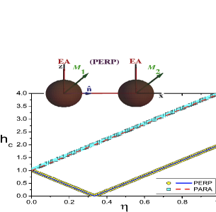
Figure 1: The (normalized) critical switching field $h_{c}$ versus the DDI strength $\eta$ for PERP and PARA configuration illustrated in the insets. Analytical results (solid and dashed lines) are compared with numerical findings (circles and squares). The system parameters are $k=0.5$ and $\alpha=0.1$.

Let us focus on two typical configurations where the connecting unit vector $\hat{n}$ is either perpendicular or parallel to the anisotropy axes, referred to as PERP and PARA configuration, respectively (see insets in Fig. 1). That is, introducing spherical coordinates $\vec{m}_{i}=(\sin\theta_{i}\cos\phi_{i},\sin\theta_{i}\sin\phi_{i},\cos\theta_{i})$, $\hat{n}=(\sin\theta_{n}\cos\phi_{n},\sin\theta_{n}\sin\phi_{n},\cos\theta_{n})$, we have $\theta_{n}=\pi/2$ for PERP configuration and $\theta_{n}=0$ for PARA (or $\theta_{n}=\pi$ since DDI is invariant under $\hat{n}\mapsto-\hat{n}$). Moreover, without loss of generality, we can let $\phi_{n}=0$ by choosing the $x$-axis along the connecting line of the two particles. Furthermore, we concentrate on the synchronized magnetic dynamics of the two Stoner particles, where both magnetization vectors remain in parallel throughout the motion, $\theta_{1}=\theta_{2}=\theta$, $\phi_{1}=\phi_{2}=\phi$. Thus, the two particles behave like a single entity, and this two-body Stoner particle can be regarded as a computer information bit. We have verified by numerical simulations (see discussion below) that this dynamical regime is stable against perturbations. For this synchronized motion mode, the nonlinear coupled LLG equations (1) read in spherical coordinates

$$\dot{\theta}+\alpha\sin\theta\dot{\phi}=-3\eta\cos\psi\sin\theta_{n}\sin\phi\,,$$

$$\alpha\dot{\theta}-\sin\theta\dot{\phi}=h\sin\theta-k\sin 2\theta+\frac{3\eta}{2}\frac{\partial\cos^{2}\psi}{\partial\theta}\,,$$ (3)

where $\psi$ is the angle between $\vec{m}$ and $\hat{n}$, i.e. $\cos\psi=\cos\theta\cos\theta_{n}+\sin\theta\sin\theta_{n}\cos\phi$. Here we have put $\vec{h}=-h\hat{z}$ (antiparallel) along the easy axis, which is the usual field configuration for reversing a magnetic bit. The above equations are the starting point of our numerical calculations to be discussed below.

However, in order to analytically explore the SW limit for magnetic reversalStoner ; llg1 , we assume the external field to lie in the plane spanned by the easy axis and the interparticle direction, $\vec{h}=h_{z}\hat{z}+h_{x}\hat{x}$. The energy takes the form $E=-2k\cos^{2}\theta-2h_{z}\cos\theta-2h_{x}\sin\theta+\eta(1-3\cos^{2}\psi)$ with $\psi=\theta-\theta_{n}$. The SW limit occurs at the inflection of the energy as a function of $\theta$, i.e. $\partial E/\partial\theta=\partial^{2}E/\partial\theta^{2}=0$. An elementary calculation translates this condition into

$$\left(\frac{h_{x}}{2k\mp 3\eta}\right)^{2/3}+\left(\frac{h_{z}}{2k\mp 3\eta}\right)^{2/3}=1,$$ (4)

where the minus(plus) sign corresponds to the PERP(PARA) configuration, respectively. Note that in the absence of DDI, $\eta=0$, the above equation just recovers the usual SW limit for a single Stoner particle. As a result, the critical switching field $h_{c}$ (applied antiparallel to the easy axis) is given by

$$h^{PERP}_{c}=|2k-3\eta|,\qquad h^{PARA}_{c}=2k+3\eta.$$ (5)

This analytical solution (5) is shown by the solid and dashed lines in Fig. 1.

Moreover, the above findings imply the remarkable observation that in the PERP configuration there exists a critical DDI strength $\eta_{c}=2k/3$ such that the critical switching field vanishes! ($h_{c}=0$).
The zero-field condition is achieved for interparticle distances given by

$$d_{c}=\left(\frac{3\mu_{0}M_{s}^{2}V}{8\pi K}\right)^{1/3},$$ (6)

where $K=k\mu_{0}M_{s}^{2}$ is the standard anisotropy coefficient. Remarkably, the above condition is independent of the damping, and its physical contents can be illustrated in terms of energy landscape. In the PERP configuration, the energy in the absence of an external field is $E=-2\eta+3(\eta-\eta_{c})\cos^{2}\theta$. Thus, for $\eta=\eta_{c}$, any angle $\theta$ represents an equilibrium position such that an arbitrary small field is sufficient to move the magnetization along the field axis, implying the possibility of zero-field reversal. Moreover, for $\eta>\eta_{c}$, the zero-field ground state is given by $\theta=\pi/2$, i.e. the synchronized magnetization points along the interparticle axis, while for $\eta<\eta_{c}$, the ground state magnetization is along the easy axis, $\theta=0,\pi$.

In order to complement and quantitatively support our previous discussion, we have performed numerical simulations of the LLG equations (3) using the 4th-order Runge-Kutta scheme. We consider a range of the DDI parameter of $0\leq\eta\leq 1$. The case, $\eta=0$ corresponds to the limit $d\rightarrow\infty$, i.e. the two nanoparticles being infinitely apart. Large $\eta$ can be realized by fabricating magnetic particles of ellipsoidal shape allowing for a closer proximity. Throughout the numerical results shown here, we use a damping parameter of $\alpha=0.1$. In Fig. 1 we compare simulation results for the critical switching field with the analytical formulae (5), both findings being in excellent agreement. The critical switching field in the PARA configuration is always higher than the value without DDI. Thus, only the PERP configuration will be useful for possible technology applications.

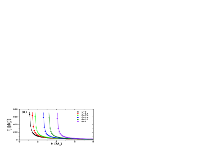
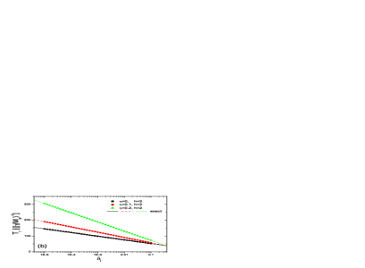
Figure 2: PARA configuration: (a) Reversal time $T_{r}$ versus field magnitude $h$ at different DDI strength $\eta$. The simulation data (symbols) is fitted according to the approximate expression $T_{r}\simeq\frac{2\lambda h(-\ln\delta_{i})}{h^{2}-h_{0}^{2}}$ for $\delta_{i}=\delta_{f}=0.001$, and $k=0.5$, $\alpha=0.1$ (cf. Fig 1). (b) Dependence of $T_{r}$ on the initial condition $\delta_{i}$: Simulation data along with exact analytical results according to Eq. (7). The final state is fixed to be $\delta_{f}=0.001$.

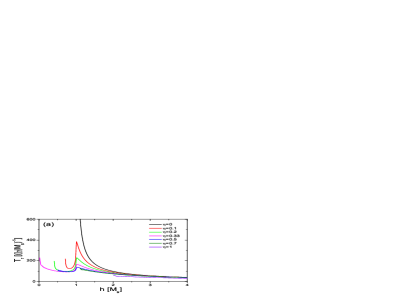
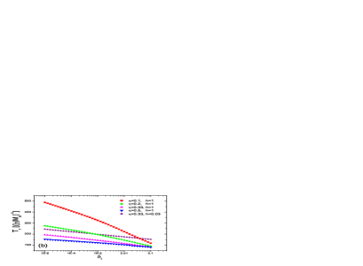
Figure 3: PERP configuration: (a) Reversal time $T_{r}$ obtained from numerical simulations versus field magnitude $h$ at different DDI strength $\eta$. (b) $T_{r}$ as a function the initial condition $\delta_{i}$. All other parameters are the same as Fig. 2.

Let us now turn to the reversal time $T_{r}$, i.e. the duration of the reversal process of the magnetization direction changing the angle $\theta$ from $0$ to $\pi$. To avoid the metastable points $\theta=0,\pi$, we introduce two small deviations $\delta_{i},\delta_{f}$, by defining $\theta_{i}=\delta_{i}$ (i.e. $m_{z}\approx 1$) and $\theta_{f}=\pi-\delta_{f}$ (i.e. $m_{z}\approx-1$), which leads to a finite reversal time in our simulations. In the PARA configuration, one can derive a closed analytical expression for this quantity,

$$T_{r}=-\lambda\left[\frac{\ln\delta_{i}}{h-h_{0}}+\frac{\ln\delta_{f}}{h+h_{0}}+\frac{h_{0}\ln(\frac{h+h_{0}}{h-h_{0}})-h\ln 4}{h^{2}-h_{0}^{2}}\right]\,,$$ (7)

where $h_{0}=2k+3\eta$ and $\lambda=(1+\alpha^{2})/\alpha$. Note that the case $\eta=0$ also includes the PERP configuration since both configurations are indistinguishable here.

In the upper panel (a) of Fig. 2 we show simulation results for $T_{r}$ in the PARA configuration for again $k=0.5$, $\delta_{i}=\delta_{f}=0.001$, and various $\eta$. The simulation data is well described by the approximate expression $T_{r}\simeq\frac{2\lambda h(-\ln\delta_{i})}{h^{2}-h_{0}^{2}}$ valid for small $\delta_{i}=\delta_{f}\ll 1$. As a result, in the PARA configuration the reversal time increases with increasing strength of the dipolar interaction. The sensitivity of the data to the parameters $\delta_{i}$ (where $\delta_{f}$ is fixed or vice versa) is illustrated in the bottom panel (b) of Fig. 2: In accordance with Eq. (7), the reversal time depends only logarithmically on the quantity and does not change its order of magnitude while $\delta_{i}$ is changing over several powers of ten. Thus our results are not qualitatively affected by our choice of the condition $\delta_{i}=\delta_{f}=0.001$.

A similar result regarding the sensitivity to initial conditions is obtained in the PERP configuration. Here an analytical result comparable to Eq. (7) does not seem to be achievable. However, the simulation data is shown in Fig. 3(b) that $T_{r}$ again depends only logarithmically on $\delta_{i}$ and is therefore similarly insensitive to the initial condition as in the PARA case.

The dependence of the reversal time on the dipolar parameter $\eta$ shown in Fig. 3(a), however, is strikingly different from the PARA configuration: Here $T_{r}$ clearly decreases with increasing $\eta$, especially in the regime of low fields, which also strongly favors the two-body bit implementation proposed in this letter.

Thus, around the critical DDI strength $\eta_{c}$ we find not only nearly a zero critical switching field but also a substantially shorter reversal time. This result promises attractive future applications for computer technology, such as fast read/write hard disk or magnetic RAM. Let us discuss two schematic setups for experimentally realizing the zero-field switching mechanism. The first scheme A is illustrated in the upper-left panel of Fig. 4, along with a numerical simulation in panel (a). Here we chose again $k=0.5$, and the DDI parameter is $\eta=0.32<\eta_{c}=1/3$. Thus, the magnetization in the zero-field ground state points along the easy axis ($z$-axis). Implementation steps of scheme A are demonstrated as follows: Step 1 - First we choose a casual initial condition, for instance $m_{1z}(0)=m_{2z}(0)=0.5$, to mimic the relaxation of the system to its ground state under zero-field during $0<t<500$; Step 2 - Then we apply a tiny antiparallel field $h=0.03$ during $500<t<1000$ which drives the magnetization reversal process of the two-body Stoner particle along the field direction. The reversal time is found to be $T_{r}\approx 198(|\gamma|M_{s})^{-1}$, and the inset shows the reversal process on a smaller scale; Step 3 - Finally we quench the field and obtain the new stable magnetic state.

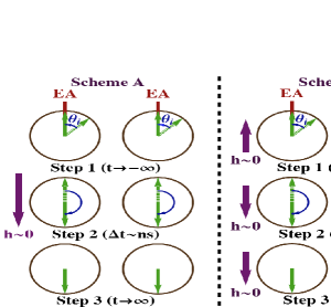
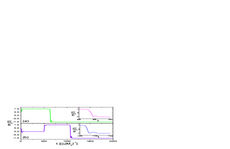
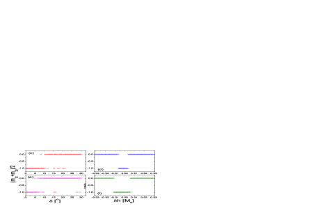
Figure 4: Upper panels: Two schemes of magnetization reversals of the two-body Stoner particle (see text).
Middle panels: $m_{z}(t)$ versus time at (a) $\eta=0.33<\eta_{c}=1/3$, (b) $\eta=0.34>\eta_{c}=1/3$. In (a), an antiparallel field $h=0.03$ is applied only during the time interval $500<t<1000$ with a reversal time of $T_{r}\approx 198(|\gamma|M_{s})^{-1}$; In (b), a parallel field $h=-0.03$ is applied during $500<t<1000$ and then reversed to $h=0.03$, leading to a reversal time as $T_{r}\approx 155(|\gamma|M_{s})^{-1}$. The insets show the reversal process on a smaller scale.
Bottom panels (c) & (e): Average stable magnetization $(m_{1z}+m_{2z})/2$ versus the deviation angle $\delta=\theta_{2}-\theta_{1}$ (in degrees) between the initial magnetization directions in the two schemes A and B, respectively. Panels (d) & (f): Analogous data as a function of the deviation field $\delta h=h_{2}-h_{1}$ antiparallel to the easy axis (see text).

The second scheme B is sketched in the upper-right panel of Fig. 4 along with a numerical simulation in middle panel (b). Here $\eta=0.34>\eta_{c}=1/3$ for $k=0.5$, i.e. the zero-field ground state is along the hard axis ($x$-direction), and a field along the easy axis is permanently required to preserve the magnetization state (information)note1 . However, our results show that such a field can be very small and actually close to zero. Thus, it is not implausible to generate such a field as the Oersted field of tiny switchable currents. The reversal process can be implemented as follows: Step 1 - We again choose the initial condition $m_{1z}(0)=m_{2z}(0)=0.5$, and the system relaxes to its ground state ($x$-axis) during $0<t<500$. Then we apply a tiny field $h=-0.03$ (note our definition $\vec{h}=-h\hat{z}$) to preserve the magnetic state $m_{z}=1$ during $500<t<1000$; Step 2 - After $t>1000$ the field is reversed to $h=0.03$, and the two-body particle reverses its magnetization during a reversal time as $T_{r}\approx 155(|\gamma|M_{s})^{-1}$ (see also inset); Step 3 - The reverse field is applied permanently to preserve the bit information.

We now address the stability of the synchronized dynamics of the two-body particle as studied so far. Let us first investigate small deviations of the initial magnetization directions of the two subparticles being otherwise still identical. In detail, we fixed the initial direction (at $t=500$ in reversal scheme A, and at $t=1000$ for scheme B) of one subparticle to be close to the $z$-axis, i.e. $\theta_{1}=0.001$, and changed the other initial direction to $\theta_{2}=0.001+\delta$. The result is shown in Fig. 4(c) and (e): For a finite range of deviations, $\delta<7.8^{\circ}$ ($\delta<4.5^{\circ}$) in scheme A(B), the synchronized mode remains stable, while for substantially larger $\delta$, the average magnetization mostly reaches zero.

Let us now consider the case where the two particles differ slightly in anisotropy $K_{i}$, volume $V_{i}$, saturation magnetization $M_{s,i}$ ($i=1,2$). Here the zero-field mechanism still occurs at $\eta_{c}=(k_{1}+k_{2})/3=\frac{2(K_{1}V_{1}+K_{2}V_{2})}{3\mu_{0}M_{s1}M_{s2}(V_{1}+V_{2})}$. However, the effective field experienced by each particle will also be slightly different. To numerically check the stability under such different external fields, we fixed the field on one subparticle to $h_{1}=0.03$ and changed the field on the other subparticle as $h_{2}=0.03+\delta h$. The numerical results are given in Fig 4(d) and (f) for reversal schemes A and B, respectively, and demonstrate again a finite range of stability against deviations from the case of strictly identical particles.

To give a concrete and practical example of our findings, let us discuss the case of cobalt (Co) particles. The standard data is $M_{s}=1400$kA/m, uniaxial strength $K=10^{5}$J/m³, $\alpha=0.1$Back . Thus $k=K/(\mu_{0}M_{s}^{2})=0.04$ such that $\eta_{c}=0.027$. For two spherical particles with radius $r$, i.e. $\eta=r^{3}/(3d^{3})$, the critical DDI strength is reached at $d_{c}=2.3r$. The critical switching field without DDI (SW limit) is $H_{SW}=2K/(\mu_{0}M_{s})=1400$Oe. In the presence of DDI, and considering deviations $\Delta d$ from $d_{c}$, one can express the critical switching field as $H_{c}/H_{SW}=3|\Delta d|/d_{c}$. Thus, in order to drastically reduce the switching field by taking advantage of our proposal, one has to engineer the interparticle distance on a scale of $d_{c}=2.3r$ which is typically a few hundred nanometers. In the case of Co, the time unit is $(|\gamma|M_{s})^{-1}\ =3.23$ps rendering the reversal times in the schemes A and B to be $T_{r}\approx 0.64$ns and $T_{r}\approx 0.5$ns, respectively, which are much shorter than in the conventional setup.

Another important issue concerns thermal fluctuations. For $\eta<\eta_{c}$ the ground state ($\theta=0,\pi$) is stable if the energy barrier in presence of DDI is large compared to the thermal energy $3(\Delta\eta)\mu_{0}M_{s}^{2}V\gg k_{B}T$ ($k_{B}$: Boltzmann’s constant), which translates for $T=400$K and the above parameters for Co into $(\Delta\eta)r^{3}\gg 0.18{\rm nm}^{3}$. On the other hand, the energy scale of the applied field should also be large compared to thermal effects, $2\mu_{0}M_{s}HV\gg k_{B}T$, which, under the same conditions, reduces to $H\gg 4700/r^{3}\,{\rm Oe}\,{\rm nm}^{3}$. Thus, considering a typical particle radius of $r=100$nm, i.e. $d_{c}=230$nm, and $H_{c}/H_{SW}=0.03$, i.e. $H_{c}=42$Oe, both conditions are easily satisfied, $(\Delta\eta)r^{3}=810{\rm nm}^{3}\gg 0.18{\rm nm}^{3}$ and $H_{c}=42$Oe $\gg 0.0047$Oe.

Finally, we would like to remark that our general results regarding the influence of dipolar interaction on the critical switching field of two-body Stoner particles are consistent with recent experimental and micromagnetic simulation results showing that the coercive field for an array of nanowires can be lower than for a single nanowireNielsch ; Hertel .

Acknowledgments– We thank Christian Back for useful discussions. This work has been supported by the Alexander von Humboldt Foundation (ZZS), by DAAD-FUNDAYACUCHO (AL), and by Deutsche Forschungsgemeinschaft via SFB 689.

References

- (1) Parkin, S. S. P., Hayashi, M. & Thomas, L. Magnetic domain-wall racetrack memory. Science 320, 190 (2008).
- (2) Allwood, D. A. et al. Magnetic domain-wall logic. Science 309, 1688 (2005).
- (3) Sun, Shouheng et al. Monodisperse FePt nanoparticles and ferromagnetic FePt nanocrystal superlattices. Science 287, 1989 (2000).
- (4) Back, C. H. et al. Minimum field strength in precessional magnetization reversal. Science 285, 864 (1999).
- (5) Schumacher, H. W. et al. Quasiballistic magnetization reversal. Phys. Rev. Lett. 90, 017204 (2003).
- (6) Thirion, C., Wernsdorfer, W. & Mailly, D. Switching of magnetization by nonlinear resonance studied in single nanoparticles. Nat. Mater. 2, 524 (2003).
- (7) Sun, Z. Z. & Wang, X. R. Fast magnetization switching of Stoner particles: A nonlinear dynamics picture. Phys. Rev. B 71, 174430 (2005).
- (8) Sun, Z. Z. & Wang, X. R. Theoretical limit of the minimal magnetization switching field and the optimal field pulse for Stoner particles. Phys. Rev. Lett. 97, 077205 (2006).
- (9) Sun, Z. Z. & Wang, X. R. Magnetization reversal through synchronization with a microwave. Phys. Rev. B 74, 132401 (2006).
- (10) Tsoi, M. et al. Excitation of a magnetic multilayer by an electric current. Phys. Rev. Lett. 80, 4281 (1998).
- (11) Sun, J. Z. Current-driven magnetic switching in manganite trilayer junctions. J. Magn. Magn. Mater. 202, 157 (1999).
- (12) Myers, E. B. et al. Current-induced switching of domains in magnetic multilayer devices. Science 285, 867 (1999).
- (13) Kiselev, S. I. et al. Microwave oscillations of a nanomagnet driven by a spin-polarized current. Nature 425, 380 (2003).
- (14) Slonczewski, J. Current-driven excitation of magnetic multilayers. J. Magn. Magn. Mater. 159, L1 (1996).
- (15) Berger, L. Emission of spin waves by a magnetic multilayer traversed by a current. Phys. Rev. B 54, 9353 (1996).
- (16) Bazaliy, Y. B., Jones, B. A. & Zhang, S.-C. Modification of the Landau-Lifshitz equation in the presence of a spin-polarized current in colossal- and giant-magnetoresistive materials. Phys. Rev. B 57, R3212 (1998).
- (17) Waintal, X., Myers, E. B., Brouwer, P. W. & Ralph, D. C. Role of spin-dependent interface scattering in generating current-induced torques in magnetic multilayers. Phys. Rev. B 62, 12317 (2000).
- (18) Brataas, A., Nazarov, Yu. V. & Bauer G. E. W. Finite-element theory of transport in ferromagnet-normal metal systems. Phys. Rev. Lett. 84, 2481 (2000).
- (19) Stiles, M. D. & Zangwill, A. Anatomy of spin-transfer torque. Phys. Rev. B 66, 014407 (2002).
- (20) Wang, X. R. & Sun, Z. Z. Theoretical limit in the magnetization reversal of Stoner particles. Phys. Rev. Lett. 98, 077201 (2007).
- (21) Landau, L. & Lifshitz, E. On the theory of the dispersion of magnetic permeability in ferromagnetic bodies. Phys. Z. Sowjetunion 8, 153 (1953).
- (22) Gilbert, T. L. A Lagrangian formulation of the gyromagnetic equation of the magnetic field. Phys. Rev. 100, 1243 (1955).
- (23) Stoner, E. C. & Wohlfarth, E. P. A mechanism of magnetic hysteresis in heterogeneous alloys. Philos. Trans. R. Soc. London A 240, 599 (1948).
- (24) One might also consider a reversal process along the hard axis to by applying a field along - direction. However, numerical simulations show that the synchronized motion mode becomes unstable for such an initial condition. This is different from the reversal process in scheme B (see text).
- (25) Nielsch, K. et al. Hexagonally ordered 100 nm period nickel nanowire arrays. Appl. Phys. Lett. 79, 1360 (2001).
- (26) Hertel, R. Computational micromagnetism of magnetization processes in nickel nanowires. J. Magn. Magn. Mater. 249, 251 (2002).