Coulomb interaction and first order superconductor-insulator transition

Abstract

The superconductor-insulator transition (SIT) in regular arrays of Josephson junctions is studied at low temperatures. Near the transition a Ginzburg-Landau type action containing the imaginary time is derived. The new feature of this action is that it contains a gauge field $\Phi$ describing the Coulomb interaction and changing the standard critical behavior. The solution of renormalization group (RG) equations derived at zero temperature $T=0$ in the space dimensionality $d=3$ shows that the SIT is always of the first order. At finite temperatures, a tricritical point separates the lines of the first and second order phase transitions. The same conclusion holds for $d=2$ if the mutual capacitance is larger than the distance between junctions.

Introduction –After several decades of intensive studies Josephson junctions arrays (JJA) still remain an important and inspiring problem. These, at first glance, simple systems exhibit, depending on parameters, superconducting, insulating or metallic properties (see for a review fazio ). As a model, JJA is relevant for granular superconductors and disordered superconducting films gantmakher .

Coulomb interaction (CI) is crucial for properties of the JJA. It suppresses the density fluctuations, i.e. causes fluctuations of phase $\varphi$ of the superconducting order parameter, which can destroy the superconductivity even at zero temperature, $T=0$. As the charging energy of one grain increases, the JJA undergoes a superconductor-insulator transition (SIT) – an example of a quantum phase transition. As we show in this Letter the long-range nature of the CI qualitatively affects the SIT.

JJA can be described by the effective Hamiltonian efetov1980

$$\hat{H}=\frac{1}{2}\sum_{{\boldmath r},{\boldmath r}^{\prime}}B_{|{\boldmath r}-{\boldmath r}^{\prime}|}\hat{n}_{{\boldmath r}}\hat{n}_{{\boldmath r}^{\prime}}-\sum_{{\boldmath r},{\boldmath r}^{\prime}}J_{{\boldmath r},{\boldmath r}^{\prime}}\cos\left(\varphi_{{\boldmath r}}-\varphi_{{\boldmath r}^{\prime}}\right),\quad$$ (1a)

where $$J_{{\boldmath r},{\boldmath r}^{\prime}} {\boldmath r} {\boldmath r}^{\prime}, \hat{n}_{{\boldmath r}} \hat{n}_{r}=-i\partial/\partial\varphi_{{\boldmath r}} +2e/(-2e) B_{r-r^{\prime}} r,r^{\prime}$$ is the Josephson energy of the junction between neighboring grains and and is the particle number operator in a grain. We assume that superconducting pairing within each grain is strong and consider the limit of the infinite single-electron gap. Accordingly, the excitations of isolated grains have the charge (bosons/antibosons). Matrix describes the interaction between two bosons on the metallic grains . It is well approximated as

$$B_{r}^{d=3}\simeq\frac{e^{2}\ell}{\pi{\cal C}r};\quad B_{r}^{d=2}\simeq\frac{2e^{2}}{\pi{\cal C}}\ln\left(\frac{2\pi{\cal C}+r}{r}\right).$$ (1b)

Here $$\ell {\cal C}\gtrsim\ell B_{0}\simeq B_{r\sim\ell}$$ is the period of JJA, and is the mutual capacitance of the neighboring grains. The energy to charge one grain can be estimated as .

Equation (1a) looks like a Hamiltonian of a quantum $XY$ -model whose critical behavior is described by an $N=2$ -component $\phi^{4}$ field theory. Such a field theory was discussed, e.g., in Refs. cha ; otterlo ; sachdev for both finite $T$ and $T=0$. For $T>0$, the critical behavior near the phase transition is described by a $d$-dimensional $2$-component $\phi^{4}$ theory: the quantum transition at $T=0$ involves imaginary time $\tau$ as an additional dimension, i.e. the same $\phi^{4}$ theory should be considered in $d+1$ dimensions. In both cases the SIT is of the second order with the critical behavior of $XY$ model in $d$ or $d+1$ dimensions.

This is correct if the matrices $B_{{\boldmath r}-{\boldmath r}^{\prime}}$ in Eq. (1b) are either diagonal, $B_{{\boldmath r},{\boldmath r}^{\prime}}^{\left(0\right)}=B_{0}\delta_{{\boldmath r},{\boldmath r}^{\prime}}$ or sufficiently short ranged. The effect of the long range part of Eq. (1b) on the critical behavior has not been investigated so far.

In this Letter we derive a field theory that properly describes the SIT at low temperatures in the disorder-free model (1). The Coulomb interaction ($1/\left|{\boldmath r}-{\boldmath r}^{\prime}\right|$ decay of $B_{r,r^{\prime}}$ at large distances) results in an additional gauge field $\Phi$ in the Ginzburg-Landau (GL) expansion near SIT and, at $T\to 0$, causes additional logarithmic divergences in the upper critical dimensionality $d=3$ of JJA. We derive and solve renormalization group (RG) equations. Solutions demonstrate the first order SIT at sufficiently low temperatures. To describe SIT in $2D$ JJA we use $\epsilon$-expansion at small $\epsilon=3-d$. We find first order SIT as long ${\cal C}\gg\ell$, and it may become continuous otherwise.

Problems with mean field description– To derive the field theory of fluctuations near the phase transitions one should write a GL expansion in superconducting order parameter $\Delta=J\left\langle\exp\left(i\varphi_{r}\right)\right\rangle,$ where $\left\langle...\right\rangle$ is the quantum mechanical average with the Hamiltonian (1a), and $J=\sum_{r}J_{r\mathbf{,}r^{\prime}}$. The mean field approximation is obtained by minimizing this expansion. At first glance, the free energy functional $F\left[\Delta\right]$ can be derived straightforwardly and should have a form of the standard GL expansion. Indeed, $F\left[\Delta\right]$ for time-independent $\Delta_{r}$ has the form

$$F\left[\Delta\right]=\sum_{{\boldmath r},{\boldmath r}^{\prime}}\left[\alpha_{{\boldmath r},{\boldmath r}^{\prime}}\Delta_{{\boldmath r}}\Delta_{{\boldmath r}^{\prime}}^{*}+\beta_{{\boldmath r},{\boldmath r}^{\prime}}\left|\Delta_{{\boldmath r}}\right|^{2}\left|\Delta_{{\boldmath r}^{\prime}}\right|^{2}\right],$$ (2a)

where the phase transition is controlled by

$$\alpha_{{\boldmath r},{\boldmath r}^{\prime}}=\left[J^{-1}\right]_{{\boldmath r},{\boldmath r}^{\prime}}-{2}\delta_{{\boldmath r},{\boldmath r}^{\prime}}/E_{0},\quad$$ (2b)

and $$E_{0}=B_{0}/2 J_{c}$$ is the energy of adding or subtracting one Cooper pair (boson) to a grain. Apparently, according Eqs. (2a)-(2b), there exists the critical coupling

$$J_{c}=E_{0}/2,$$ (2c)

so that at $$J>J_{c} J<J_{c} \beta_{{\boldmath r},{\boldmath r}^{\prime}}$$ the system is a superconductor, while the insulating state corresponds to . However, this conclusion relies on a quartic term being local and positive. Explicit calculation of the function starting from Eq. (1a) gives eckern

$$\beta_{{\boldmath r},{\boldmath r}^{\prime}}=\frac{1}{E_{0}^{3}}\left[\frac{7}{2}\delta_{{\boldmath r},{\boldmath r}^{\prime}}-4\left(\frac{E_{0}}{E_{{\boldmath r},{\boldmath r}^{\prime}}^{-}}+\frac{E_{0}}{E_{{\boldmath r},{\boldmath r}^{\prime}}^{+}}-1\right)\right],$$ (2d)

where $$E_{{\boldmath r},{\boldmath r}^{\prime}}^{\pm}=B_{0}\pm B_{{\boldmath r},{\boldmath r}^{\prime}} r r^{\prime} B_{r,r^{\prime}}\ll B_{0}$$ are the energies of two bosons (boson-antiboson) pairs located on the grains and . At large distances , and Eq. (2d) yields

$$\beta_{|r-r^{\prime}|\gg\ell}=-B_{r,r^{\prime}}^{2}/E_{0}^{5},$$ (2e)

As at large distances $$B_{r,r^{\prime}}\propto\left|r-r^{\prime}\right|^{-1} r^{\prime} \left|\Delta\right| 3(2) T\ll E_{0}, T\gg E_{0}$$, the sum over in Eq. (2a) is negative and diverges linearly (logarithmically) for coordinate-independent in -dimensional JJAs. Such divergences at large distances signal that the additional soft modes should be included to make the theory local, and the conventional naive mean-field is not conclusive. This problem arises at low temperatures, only, while for , the Coulomb interaction can be neglected and the SIT temperature in the mean-field approximation efetov1980 turns out to be

$$T_{c}=J.$$ (3)

In the vicinity of $T_{c}$ the conventional GL free energy with a time-independent $\Delta$ is valid.

Effective field theory– To account for the long range interaction we modify the model slightly: we separate $B_{r,r^{\prime}}$ Eq. (1b) into the local and long-range parts and smoothen the latter:

$$B_{{\boldmath r}}\simeq 2E_{0}\delta_{{\boldmath r},0}+{B}_{|{\boldmath r}|+\gamma l},\$$ (4)

where $\gamma\gtrsim 1$ which controls the short distance cut-off that will drop out of final results. Although we assume $E_{0}\gg\ell\partial_{r}{B}_{|{\boldmath r}|}|_{r\simeq\ell}$, the number of long range terms is infinite and their effect accumulated from large distances has to be included together with quantum fluctuations of $\Delta$. We separate the Hamiltonian into the bare one, $H_{0}$, and perturbations $H_{J,B}$

$$\begin{split}&\hat{H}=\hat{H}_{0}+\hat{H}_{J}+\hat{H}_{B},\quad\hat{H}_{0}=\sum_{{\boldmath r}}E_{0}\hat{n}_{r}^{2},\\ &\hat{H}_{B}=\sum_{r,r^{\prime}}\frac{\tilde{B}_{{\boldmath r},{\boldmath r}^{\prime}}\hat{n}_{{\boldmath r}}\hat{n}_{{\boldmath r}^{\prime}}}{2},\quad\hat{H}_{J}=-\sum_{r,r^{\prime}}J_{r,r^{\prime}}\cos\left(\hat{\varphi}_{r}-\hat{\varphi}_{r^{\prime}}\right),\end{split}$$ (5)

and write the partition function

$${Z}=Tr\ e^{-\hat{H}/T}Z_{0}\left\langle T_{\tau}e^{-\int_{0}^{1/T}d\tau\left[\hat{H}_{J}\left(\tau\right)+\hat{H}_{B}\left(\tau\right)\right]}\right\rangle_{0}.$$ (6)

Here $T_{\tau}$ stands for imaginary time ordering, $\left\langle\dots\right\rangle_{0}\equiv{Z_{0}}^{-1}Tr\left\{e^{-\hat{H}_{0}}/T\dots\right\}$, $Z_{0}=Tr\left\{e^{-\hat{H}_{0}}/T\right\}$, and $\hat{H}_{B,\,J}\left(\tau\right)\equiv e^{\hat{H}_{0}\tau}\hat{H}_{B,\,J}e^{-\hat{H}_{0}\tau}$. Terms $\hat{H}_{B}\left(\tau\right)$ and $\hat{H}_{J}\left(\tau\right)$ are decoupled by Hubbard-Stratonovich fields $\Delta_{{\boldmath r}}\left(\tau\right)$ (complex) and $\Phi_{r}\left(\tau\right)$ (real):

$$\begin{split}&\frac{Z}{Z_{0}}=\!\int\!\!{\cal D}\Delta_{\boldmath r}{\cal D}\Delta^{\ast}_{\boldmath r}{\cal D}\Phi_{\boldmath r}e^{-S_{1}}\left\langle T_{\tau}e^{-\int_{0}^{1/T}\hat{H}_{1}d\tau}\right\rangle_{0},\\ &\hat{H}_{1}=\sum_{{\boldmath r}}\Big{\{}i\left[\hat{n}_{{\boldmath r}}\Phi_{{\boldmath r}}\right](\tau)+\left[\Delta_{{\boldmath r}}e^{-i\hat{\varphi}_{{\boldmath r}}}\right]\left(\tau\right)+\left[\Delta_{{\boldmath r}}^{\ast}e^{i\hat{\varphi}_{{\boldmath r}}}\right]\left(\tau\right)\Big{\}},\\ &S_{1}=\sum_{r,r^{\prime}}\int_{0}^{1/T}d\tau\left\{J_{r,r^{\prime}}^{-1}\left[\Delta_{r}\Delta_{r^{\prime}}^{\ast}\right](\tau)+\frac{1}{2}\tilde{B}_{r,r^{\prime}}^{-1}\left[\Phi_{r}\Phi_{r^{\prime}}\right](\tau)\right\},\end{split}$$ (7)

where $\sum_{r^{\prime}}\tilde{B}_{r,r^{\prime}}^{-1}B_{|r^{\prime}|+\gamma\ell}=\delta_{{\boldmath r},0}$.

In the limit of low temperatures $T\ll E_{0}$ the average $\left\langle...\right\rangle_{0}$ can be calculated over the ground state when all grains are neutral. We neglect exponentially small contributions like $\exp\left(-E_{i}/T\right),$ where $E_{i}$ are the eigenenergies of Hamiltonian $\hat{H}_{0}$ corresponding to the charged isolated grains. At the same time, we keep finite $1/T$ when integrating over $\tau$ in Eqs. (7) to obtain algebraic in $T$ contributions. This calculation is carried out near the SIT by cumulant expansion assuming that the fields $\Delta\left(\tau,{\boldmath r}\right),\Phi(\tau,{\boldmath r})$ are slow in both time $\tau$ and coordinate $r$. As we compute averages with the bare Hamiltonian $\hat{H}_{0}$, all generated terms remain local. Introducing continuous coordinate description we obtain

$$Z\!=\!\int e^{-\int_{0}^{1/T}d\tau(L_{\Delta}+L_{\Phi})}{\cal D}\Delta({\boldmath r},\tau){\cal D}\Delta^{\ast}({\boldmath r},\tau){\cal D}\Phi({\boldmath r},\tau).$$ (8a)

The order parameter is controlled by Lagrangian

$$\begin{split}L_{\Delta}=\int d^{d}r&\Big{\{}f^{2}\Delta^{*}\left[aE^{2}-\left(\partial_{\tau}+i\Phi\right)^{2}-c^{2}\nabla^{2}\right]\Delta\\ &+bf^{4}\pi^{2}c^{d}E^{\epsilon}\left|\Delta\right|^{4}\Big{\}},\end{split}$$ (8b)

where $$\epsilon\equiv 3-d |\delta J|\ll J_{c}=E_{0}/2;\delta J=J-J_{c}$$. The coefficients in this action are expressed in terms of the initial constants of the Hamiltonian (5) at , as

$$c^{2}\!=\frac{E_{0}^{2}\ell^{2}}{2d};\ a=-\frac{2\delta J}{E_{0}};\ f^{2}\!=\frac{2}{E_{0}^{3}\ell^{d}};\ b=\frac{7\!\left({2d}\right)^{d/2}}{8\pi^{2}}.$$ (8c)

Energy $$E E=E_{0} (r,\tau) f \Delta a,b,c$$ is the running high-frequency cut-off in the theory, it starts at . We included this cut-off explicitly in the action to keep the interaction constants dimensionless, avoid rescaling of during RG, and explicitly illuminate the dimensionality of the interaction terms. As can be always removed by the rescaling of , the physical results may depend only on constants .

The fluctuating voltage $\Phi/\left(2e\right)$ is of great importance for the critical behavior. This field is controlled by the Gaussian Lagrangian

$$L_{\Phi}=\frac{1}{2}\int drdr^{\prime}\Phi\left(\tau,{\boldmath r}\right)\left[\tilde{B}^{-1}\right]_{{\boldmath r},{\boldmath r}^{\prime}}\Phi\left(\tau,{\boldmath r}^{\prime}\right);$$ (8d)

After the coordinate Fourier transform of the fields $\Phi(k,\tau)=\Phi^{*}({-k,\tau})$, we obtain from Eq. (1b):

$$L_{\Phi}=\!\int\!\frac{d^{d}k}{(2\pi)^{d}}|\Phi(\tau,k)|^{2}\left(\frac{g_{1}|k|^{d-1}}{8\pi^{2}c}+\frac{g_{2}k^{2}E_{0}^{-\epsilon}}{8\pi^{2}c^{d-2}}\right).$$ (8e)

Harmonics $\Phi(k)$ with $|k|\gtrsim 1/(\gamma\ell)$ are suppressed. The coupling constants in Eq. (8e) are defined as

$$\begin{split}&g_{1}^{d=3}=\left(\frac{\pi^{2}{\cal C}E_{0}}{\sqrt{6}e^{2}}\right);\quad g_{1}^{d=2}=\left(\frac{\pi\ell E_{0}}{4e^{2}}\right);\\ &g_{2}^{d=3}=0;\quad g_{2}^{d=2}=\left(\frac{\pi^{2}E_{0}{\cal C}}{e^{2}}\right).\end{split}$$ (8f)

For this approach to be applicable, the fluctuations of $\Phi$ should be small i.e. $g_{1}+g_{2}\gtrsim 1$.

The field theory (8) defined for two slow fields $\Delta,\Phi$ helps one to avoid the negative and non-local quartic terms Eq. (2e), arising in a single field formulation (2a). Indeed, Eqs. (8) are invariant under the transformation

$$\Phi_{r}\left(\tau\right)\rightarrow\Phi_{r}\left(\tau\right)+\phi(\tau);\quad\Delta\to\Delta e^{-i\int_{0}^{\tau}d\tau_{1}\phi(\tau_{1})}$$ (9)

for $\int_{0}^{\beta}\phi(\tau)d\tau=0\,(\!\!\!\!\mod 2\pi)$, i.e. the effect of the fluctuations of $\Phi_{k}e^{i\omega\tau}$ at $kc\ll\omega$ vanishes. Fixing by hand $\Delta$ while allowing for all the fluctuations of $\Phi$ violates the gauge invariance (9), and overestimates the contributions of small $k$ and leads to an incorrect non-local theory.

Renormalization group analysis– To the best of our knowledge, the model (8) has never been discussed. We analyze it using the RG approach in $d=3$ and $d=3-\epsilon$.

The cut-off dependence, $E^{\epsilon}_{0}$. in Eqs. (8b), (8e) suggests that the theory is logarithmic for $d=3$ and $a=0$. As long as $E_{0}\gtrsim T$, $\tau$ can be considered as an extra dimension and the gauge invariance (9) prohibits generating a relevant term $\propto\Phi^{2}$. The other possible terms allowed by symmetry are irrelevant, i.e. the theory is re-normalizable. For $\epsilon=1$, Eqs. (8c) and (8e) still contain all the relevant terms. Moreover, term $\propto g_{1}/c$ describes the long range Coulomb interaction and cannot be re-normalized. The term $\propto g_{2}$ is leading irrelevant and it describes the logarithmic interaction and its renormalization due to the virtual boson-antiboson pairs.

We subdivide the fields $\Delta$ and $\Phi$ into slow $\tilde{\Delta},\tilde{\Phi}$ and fast $\Delta_{0},\Phi_{0}$ parts (In the first loop approximation cut-off procedure can be rather arbitrary, we treat energy $E_{0}$ as a running cut-off), integrate in Eq. (8a) over $\Delta_{0},\Phi_{0}$ making a cumulant expansion in $\tilde{\Delta},\tilde{\Phi}$ up to the fourth order. The action is reproduced with the couplings running as

$$\frac{d{a}}{dl}=\left\{a\left(2-\frac{{b}}{2}\right)\right\}+\frac{3a}{2}\frac{1}{{g}_{1}+{g}_{2}};$$ (10a)

$$\frac{d{b}}{dl}=\left\{\epsilon{b}-\frac{5}{4}{b}^{2}\right\}-\frac{2}{\left({g}_{1}+{g}_{2}\right)^{2}}+\frac{{b}}{{g}_{1}+{g}_{2}};$$ (10b)

$$\frac{d{c}}{dl}=\frac{2}{3}\frac{c}{{g}_{1}+{g}_{2}};$$ (10c)

$$\frac{d{g}_{1}}{dl}=\frac{2}{3}\frac{{g}_{1}}{{g}_{1}+{g}_{2}};$$ (10d)

$$\frac{d{g}_{2}}{dl}=-\epsilon{g}_{2}+\frac{2}{3}\frac{{g}_{2}}{{g}_{1}+{g}_{2}}+\frac{1}{6}$$ (10e)

(the running of $f$ is of no consequence). Here

$$l=\ln\left({{\bar{B}}}/{E}_{0}\right),$$ (11)

and Eqs. (8c), (8f) are the initial conditions for Eqs. (10). The terms in curly brackets correspond to the $\beta$-function for $XY$ model in $d+1$ dimension.

RG flow should be stopped at $l\gtrsim l_{*}$,

$$l_{*}={\mathrm{m}ax}\left(l_{t};l_{a}\right);\ \ \left|a\left(l_{a}\right)\right|\simeq 1,\ \ l_{T}\simeq\ln({\bar{B}}/{T}),$$ (12)

where the quantum fluctuations loose importance either due to the finite temperature ($l_{*}=l_{T}$) or to departure from the phase transition line ($l_{*}=l_{a}$). In the former case the quantum RG analysis (in $d+1$ dimensions) should be supplemented by the analysis of the $d$-dimensional classical fluctuations.

This analysis deserves some discussion. Let us obtain the free energy from Eqs. (8b) and (8e) by including only time independent fields:

$$\begin{split}F&=\int d^{d}r\Big{\{}c^{2}_{T}\left|\nabla\Delta\right|^{2}+a_{T}T^{2}\left|\Delta\right|^{2}+b_{T}\pi^{2}c^{d}_{T}T^{\epsilon}\left|\Delta\right|^{4}\Big{\}}\\ &+\int d^{d}r\left|\Delta\right|^{2}\Phi^{2}\\ &+\!\int\!\frac{d^{d}k}{(2\pi)^{d}}\frac{|k|^{d-1}|\Phi(k)|^{2}}{{4\pi^{2}c_{T}}}\left[g_{1,T}+g_{2,T}\left(\frac{c_{T}k}{T}\right)^{\epsilon}\right],\end{split}$$ (13)

where the subscript $T$ means that the couplings are calculated at $l=l_{T}$. To obtain the canonical form one has to integrate $e^{-F/T}$ over all the configuration of $\Phi$. Such integration would immediately produce the term $\simeq-|\Delta|^{3}$ resulting in the first order phase transition. Similar effect of the fluctuating magnetic field was studied long agohlm .

However, the electrostatic potential is very different from the vector potential of the magnetic field. The gauge invariance prohibits the screening of the static vector potential by the fluctuations of $\Delta$. On the contrary, the static electrostatic potential can be screened [gauge invariance (9) does not allow to remove zero Matsubara component of $\Phi({\boldmath r})$.] Explicit calculation of the static polarization operator adds extra term

$$F_{scr}=\frac{1}{6T}\left(\frac{T}{c_{T}}\right)^{d}\int\left|\Phi_{k}\right|^{2}\frac{d^{d}k}{\left(2\pi\right)^{d}},$$ (14)

to the free energy $F$ [this term is an effect of finite $\tau$ and does not appear in RG analysis (10)]. As the result, the long-range fluctuations of $\Phi$ are massive, the last two lines in Eq. (18) can be neglected and we are left with a classical $XY$-model in $d$ dimensions. The phase transition is of the second order in $d=3$ and Berezinskii-Kosterlitz-Thouless in $d=2$. Transition temperature estimated as

$$T_{c}=\bar{B}e^{-l_{c}};\quad a\left(l_{c}\right)\simeq-b\left(l_{c}\right);$$ (15)

is shown by solid line on Fig. 1.

First order phase transition at $d=3$– Second order phase transition (15) implies $b>0$, so that the energy

$$U_{T}(|\Delta|)\simeq a(l_{\cal E}){\cal E}^{2}|\Delta|^{2}+\pi^{2}c(l_{\cal E})^{d}b(l_{\cal E})|\Delta|^{4},\$$ (16)

with ${\cal E}={\mathrm{m}ax}(T,|\Delta|),\ l_{\cal E}=\ln\frac{\bar{B}}{\cal E}$ has a single minimum.

In what follows, we solve the RG equations (10) and show that at some value of $l_{t}$, $b\left(l_{t}\right)=0$. It means, that at $T<T_{t}=\bar{B}\exp(-l_{t})$ the additional stable minimum appear in Eq. (16); the transition is of the first order – theory is massive and renormalization terminates. The vicinity of $T_{t}$ can be analyzed in the spirit of Ref. wegner .

For $d=3$ only ${g}={g}_{1}+{g}_{2}$ is important and we find

$$\begin{split}{g}\left(l\right)=\frac{5\xi}{6},\ \ {b}\left(l\right)=\frac{1}{\xi}{\cal F}\left(\ln\frac{\xi}{\xi^{*}}\right),\ \ \xi=l+\frac{6g_{1}^{d=3}}{5},\end{split}$$ (17)

where $g_{1}^{d=3},b$ are given by Eqs. (8c,8f), and $\xi^{*}$ is found from $6g_{1}^{d=3}b/5={\cal F}[\ln(6g_{1}^{d=3}/5\xi^{*})].$ Function

$${\cal F}(x)=\frac{22}{25}+\frac{2\sqrt{239}}{25}\cot\left(\frac{\sqrt{239}}{10}x\right)$$ (18)

changes sign at $x\approx-0.62\dots$. Therefore, $b$ changes the sign at finite $l_{t}$ independently on the initial conditions, see Fig. 1a. As the initial couplings, $g_{1}^{d=3}\gtrsim 1,\ b\lesssim 1$ the region of the possible phase coexistence, see Fig. 1, occupies significant part of the phase diagrams.

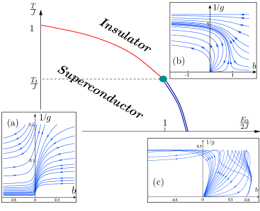
Figure 1: Phase diagram of the JJA. The solid and double- lines are the second and first order respectively. Insets: (a) the two parameter RG flow for 3D JJA; (b) two parameter RG flow for 2D arrays with logarithmic interaction; (c) the projection of three parameter RG flow for the logarithmic and “moderate” Coulomb interaction $g_{1}(l=0)=0.65$.

First order phase transition at $d=2$– The extrapolation of RG equations to $\epsilon=1$ shows that for a weak Coulomb interaction, $g_{1}^{d=2}\gg 1$, RG flow has a stable fixed point, i.e. the SIT is of the second order. Indeed, for this case $g_{1}(l)=2l/3+const$, $g_{2}\to\epsilon/6$. Then, $b$ tends to its fixed point value as $b\approx 4\epsilon/5+{\cal O}(1/g_{1})$ and the effect of the Coulomb interaction vanishes at $l\to\infty$. Therefore, the effect of the Coulomb interaction may lead only to the logarithmic corrections to the usual power laws of $d=3$ classical $XY$ model.

Situation changes in the opposite limit when the mutual capacitance significantly exceeds the intergrain distance i.e. $g_{2}\gg g_{1}$. We can set in Eqs. (10) $g_{1}=0$, then $g_{2}$ rapidly reaches its fixed point $5/6\epsilon$ and for $\epsilon=1$ evolution of $b(l)$ is governed by function (18):

$$b(l)={\cal F}\left(l+l_{*}\right);\ b_{*}={\cal F}\left(l_{*}\right),$$ (19)

where $b_{*}\sim bg_{2}$. Accordingly, $b$ always changes sign and the SIT is of the first order at $T<T_{t}\simeq E_{0}e^{-|l_{*}|}$, see Fig. 1b. If the Coulomb interaction is moderate, $g_{2}\simeq g_{1}$, both kind of phase transitions are possible, see Fig. 1c.

Physical interpretation – The stability of both insulating and superconducting states at $T<T_{t}$ appears due to the competition of the effects of the long range interaction of excitations against their Bose statistics. When the former is strong enough there exists a state formed by boson/antiboson dipoles. This stable state competes with the formation of the uniform Bose-condensate.

In conclusion we have derived an effective field theory describing the SIT transition in granular superconductors and JJA. The RG analysis of this model demonstrated that the SIT is inevitably of first order at low temperatures for all 3-dimensional and realistic 2-dimensional JJA. This may have very important experimental consequences. In particular, one can see hysteresis when changing e.g. magnetic field. The insulating and superconducting state can coexist and phase separation in space, especially in the presence of disorder, is possible. All these interesting phenomena deserve a separate study.

Support by US DOE contract No. DE- AC02-06CH11357 (I.L.A. and B.L.A.) and Transregio 12 of DFG ( S.V.S. and K.B.E.) is gratefully acknowledged.

References

• (1) R. Fazio and H. van der Zant, Phys. Rep. 355, 235 (2001)
• (2) V.F. Gantmakher and V.T. Dolgopolov, Usp. Fiz. Nauk 53, 1 (2010)
• (3) K.B. Efetov, Zh. Eksp. Teor. Fiz. 78, 2017 (1980) [Sov. Phys. JETP 51, 1015 (1980)]
• (4) M.-C. Cha et al, Phys. Rev. B 44, 6883 (1991)
• (5) A. van Otterlo et al, Phys. Rev. B 48, 3316 (1993)
• (6) K. Damle and S. Sachdev, Phys. Rev. B 56, 8714 (1997)
• (7) J.G. Kissner and U. Eckern, Z. Phys. B 91, 155 (1993)
• (8) J.E. Mooji et al, Phys. Rev. Lett. 65, 645 (1990)
• (9) B. I. Halperin, T. C. Lubensky, and S.K. Ma, Phys. Rev. Lett. 32, 292 (1974)
• (10) E. K. Riedel and F. J. Wegner, Phys. Rev. Lett., 29, 349 (1972)