Dimension of the boundary in different metrics

Abstract.

We consider metrics on Euclidean domains $\Omega\subset\mathbb{R}^{n}$ that are induced by continuous densities $\rho\colon\Omega\rightarrow(0,\infty)$ and study the Hausdorff and packing dimensions of the boundary of $\Omega$ with respect to these metrics.

1. Introduction

Let $\Omega\subset\mathbb{R}^{n}$ be a domain. For $x,y\in\Omega$, we denote by $d(x,y)$ the internal Euclidean distance between $x$ and $y$ defined as

$$d(x,y)=\inf_{\gamma}\operatorname{\ell}(\gamma),$$

where the infimum is taken over all rectifiable curves in $\Omega$ with endpoints $x$ and $y$ and $\operatorname{\ell}$ refers to the standard Euclidean length. It is well known and easy to see that $d$ defines a metric on $\Omega$ called the internal metric. Furthermore, we may extend this metric to the internal boundary $\partial\Omega_{d}=\overline{\Omega}_{d}\setminus{\Omega}$, where $\overline{\Omega}_{d}$ is the standard metric completion of $\Omega$ with respect to $d$.

Let $\rho\colon\Omega\rightarrow(0,\infty)$ be a continuous function. We define the $\rho$-length of a rectifiable curve $\gamma\subset\Omega$ as

$$\operatorname{\ell}_{\rho}(\gamma)=\int_{\gamma}\rho(z)|dz|$$

where $|dz|$ denotes integration with respect to arclength. The $\rho$-distance between $x,y\in\Omega$ is then given by

$$d_{\rho}(x,y)=\inf_{\gamma}\operatorname{\ell}_{\rho}(\gamma),$$

where the infimum is again over all curves joining $x$ to $y$ in $\Omega$. This defines a metric on $\Omega$ and as with the internal metric, we may extend it to the $\rho$-boundary of $\Omega$ defined as $\partial_{\rho}\Omega=\overline{\Omega}_{\rho}\setminus\Omega$, where $\overline{\Omega}_{\rho}$ is the standard metric completion of $\Omega$ with respect to $d_{\rho}$. Observe that the internal metric $d$ corresponds to $d_{\rho}$ for the constant function $\rho\equiv 1$.

Thus, given $\rho$ as above (a density in what follows), we have two complete metric spaces $(\overline{\Omega}_{d},d)$ and $(\overline{\Omega}_{\rho},d_{\rho})$ which need not be topologically equivalent. For simplicity, however, we only deal with cases in which $\partial_{\rho}\Omega$ may be naturally identified with a metric subspace of $\partial\Omega_{d}$.

In this paper, we will consider $\dim_{\rho}(\partial_{\rho}\Omega)$ and $\operatorname{Dim}_{\rho}(\partial_{\rho}\Omega)$, the Hausdorff and packing dimensions of $\partial_{\rho}\Omega$ with respect to $d_{\rho}$ (For more comprehensive notation and definitions, we refer to Section 2 below). Classically, this sort of problems arise in connection to harmonic measures and the boundary behaviour of conformal maps [8, 9, 13, 5, 7]. In that setting, $\rho=|f^{\prime}|$ for a conformal map $f$ and $d_{\rho}$ corresponds to the internal metric on the image domain. The Hausdorff dimension, $\dim_{\rho}(\partial_{\rho}\Omega)$, has been analysed also for a much larger collection of so called conformal densities on the unit ball $\mathbb{B}^{n}\subset\mathbb{R}^{n}$. See [2, 1, 11]. Although we provide some estimates in the setting of conformal densities, our main goal is to study general densities defined on John domains in $\mathbb{R}^{n}$, and to provide tools to estimate the values of the dimensions $\dim_{\rho}(\partial_{\rho}\Omega)$ and $\operatorname{Dim}_{\rho}(\partial_{\rho}\Omega)$. Because of this, our methods are perhaps more geometric than analytic.

Given $A\subset\overline{\Omega}_{d}$, we denote by $d(x,A)=\inf_{a\in A}d(x,a)$ the internal distance from $x$ to $A$ and, moreover, abbreviate $d(x)=d(x,\partial\Omega_{d})$. Of course, $d(x)$ is just the Euclidean distance to the boundary of $\Omega$.

Let us consider the following simple example: Suppose that $\Omega\subsetneq\mathbb{R}^{n}$ has smooth boundary, $-1<\beta<0$, and define a density $\rho(x)=d(x)^{\beta}$. Then it is well known, and easy to see that $\partial_{\rho}\Omega$ is a “snowflake”. More precisely, $d_{\rho}(x,y)\approx d(x,y)^{1+\beta}$ for all $x,y\in\partial_{\rho}\Omega$. Thus, the effect of $\rho$ on the dimensions of the boundary is described by a power law

$$\operatorname{Dim}_{d}(\partial\Omega_{d})/\operatorname{Dim}_{\rho}(\partial_{\rho}\Omega)=\dim_{d}(\partial\Omega_{d})/\dim_{\rho}(\partial_{\rho}\Omega)=1+\log\rho(x)/\log d(x).$$

Keeping this example in mind, it is now natural to consider (the upper and lower) limits of the quantity $\log\rho(y)/\log d(y)$ as $y$ approaches the boundary of $\Omega$. Under sufficient assumptions, this leads to multifractal type formulas for the dimension of $\partial_{\rho}\Omega$. For instance, we obtain the following result.

Theorem 1.1.

Let $\Omega\subset\mathbb{R}^{n}$ be a John domain and $\rho>c>0$ a density. Suppose that

$$i(x)=\lim_{y\in\Omega,\,y\rightarrow x}\frac{\log\rho(y)}{\log d(y)}$$

exists at all points $x\in\partial\Omega_{d}$ and satisfies $i(x)>-1$. Then

$$\dim_{\rho}(\partial_{\rho}\Omega)=\sup_{\beta>-1}(1+\beta)^{-1}\dim_{d}(\{x\in\partial\Omega_{d}\,:i(x)\leq\beta\})$$

An analogous formula holds for the packing dimension.

This theorem is a simple special case of a more general result, Theorem 4.2, and it can be used to obtain a formula for the dimensions $\dim_{\rho}(\partial_{\rho}\Omega)$ and $\operatorname{Dim}_{\rho}(\partial_{\rho}\Omega)$ in many situations. A generic case is the following: $\Omega=\mathbb{B}^{n}$, $C\subset\partial\mathbb{B}^{n}$ is a Cantor set with $0<\dim_{d}C<\operatorname{Dim}_{d}C<n$ and $\rho(x)=d(x,C)^{\beta}$ for some $\beta>-1$ (Example 4.4).

In Theorem 1.1, there is an annoying lack of generality since we have to consider inner limits in the definition of $i(x)$. The situation is different if we know that the distance $d_{\rho}(x,y)$ between points $x,y\in\partial_{\rho}\Omega$ is realised along curves that are “non-tangential”. If the density satisfies a suitable Harnack inequality together with a Gehring-Hayman type estimate, then it is enough to consider limits along some fixed cones. For conformal densities, for instance, we may replace the quantity $i(x)$ by a radial version $k(x)=\lim_{t\uparrow 1}\log\rho(tx)/\log(1-t)$; see Section 5 where we actually consider upper and lower limits as $t\uparrow 1$.

Section 6 contains several examples and some open questions. Most notably, in Example 6.3 we construct a new nontrivial example of a conformal density with multifractal type boundary behavior.

As our results indicate, a careful inspection of the power exponents and the size of certain sub and super level sets of these quantities can be used to study the dimensions $\dim_{\rho}(\partial_{\rho}\Omega)$ and $\operatorname{Dim}_{\rho}(\partial_{\rho}\Omega)$. Although the main idea in most of our results is the same, it is perhaps not possible to find a general statement which would fit into all, or even most, of the interesting situations. Often, a suitable case study and a combination of different ideas is needed in order to deduce the relevant information (for instance, see Examples 4.7, 6.2, and 6.3). We strongly believe that the ideas we have used can be applied also elsewhere, beyond the results of this paper.

2. Notation

Let $\Omega\subset\mathbb{R}^{n}$ be a domain. For technical reasons, we want to be able to naturally identify $\partial_{\rho}\Omega$ with a subset of $\partial\Omega_{d}$. To ensure this, we assume throughout this paper that for all sequences $(x_{i})$, $x_{i}\in\Omega$, the following two conditions are satisfied:

(A1) $$\text{If }(x_{i})\text{ converges in }\overline{\Omega}_{\rho},\text{ then it converges in }\overline{\Omega}_{d}.$$

(A2) $$\text{If }(x_{i})\text{ converges in }\overline{\Omega}_{d},\text{ it has at most one accumulation point in }\partial_{\rho}\Omega.$$

In other words, (A1) means that the identity mapping $(\Omega,d_{\rho})\to(\Omega,d)$ has a continuous extension $f\colon\overline{\Omega}_{\rho}\to\overline{\Omega}_{d}$ and, furthermore, (A2) means that this $f$ is injective.

Definition 2.1.

A density is a continuous function $\rho\colon\Omega\rightarrow(0,\infty)$ satisfying (A1) and (A2). For simplicity, we also require that $\partial_{\rho}\Omega\neq\emptyset$.

Whenever we talk about a curve $\gamma$, we assume that it is rectifiable, is arc-length parametrized, and that $\gamma(t)\in\Omega$ for all $0<t<\operatorname{\ell}(\gamma)$ (the endpoints may or may not belong to $\partial\Omega_{d}$). Note that the internal length of a curve equals the Euclidean length of the curve. We say that $\Omega\subset\mathbb{R}^{n}$ is an $\alpha$-John domain for $0<\alpha\leq 1$, if there is $x_{0}\in\Omega$ such that all points $x\in\Omega$ may be joined to $x_{0}$ by an $\alpha$-cone, i.e. by a curve $\gamma$ joining $x$ to $x_{0}$ such that $d(\gamma(t))\geq\alpha\,t$ for all $0\leq t\leq\operatorname{\ell}(\gamma)$. If $\alpha$ is not important, we simply talk about John domains. Let $\gamma\subset\Omega$ be a curve. We say that $\gamma$ is an $\alpha$-cigar if

(2.1) $$d(\gamma(t))\geq\alpha\min\{t,\operatorname{\ell}(\gamma)-t\}\text{ for all }0\leq t\leq\operatorname{\ell}(\gamma).$$

For technical purposes, we define an $\alpha$-distance between points $x,y\in\Omega$ as

$$d_{\alpha}(x,y)=\inf_{\gamma}\operatorname{\ell}(\gamma)$$

and this time the infimum is taken over all $\alpha$-cigars $\gamma$ joining $x$ and $y$. It is easy to see that if $\Omega$ is an $\alpha$-John domain, then any two points $x,y\in\overline{\Omega}_{d}$ may be joined by an $\alpha$-cigar. Thus $d_{\alpha}(x,y)<\infty$ for all $x,y\in\overline{\Omega}_{d}$. Note however that $d_{\alpha}$ is not necessarily a metric since it may be infinite and even if it happens to be finite, it may fail to satisfy the triangle inequality.

Let $X=(X,d_{X})$ be a separable metric space. We denote balls $B_{X}(x,r)=\{y\in X\,:\,d_{X}(y,x)<r\}$ and spheres $S_{X}(x,r)=\{y\in X\,:\,d_{X}(x,y)=r\}$. Given $A\subset X$, we define its $s$-dimensional Hausdorff and packing measures, $\mathcal{H}^{s}_{X}(A)$ and $\mathcal{P}^{s}_{X}(A)$, respectively, by the following procedure:

$$\mathcal{H}^{s,\varepsilon}_{X}(A) =\inf\left\{\sum_{i=1}^{\infty}\operatorname{diam}_{X}(A_{i})^{s}\colon A\subset\bigcup_{i\in\mathbb{N}}A_{i}\text{ and }\operatorname{diam}_{X}(A_{i})<\varepsilon\text{ for all }i\right\},$$

$$\mathcal{H}^{s}_{X}(A) =\lim_{\varepsilon\downarrow 0}\mathcal{H}^{s,\varepsilon}_{X}(A),$$

$$P^{s,\varepsilon}_{X}(A) =\sup\left\{\sum_{i=1}^{\infty}r_{i}^{s}\colon\{B_{X}(x_{i},r_{i})\}\text{ is a packing of }A\text{ with }r_{i}\leq\varepsilon\right\},$$

$$P^{s}_{X}(A) =\lim_{\varepsilon\downarrow 0}P^{s,\varepsilon}_{X}(A),$$

$$\mathcal{P}^{s}_{X}(A) =\inf\left\{\sum_{i=1}^{\infty}P^{s}_{X}(A_{i})\colon A\subset\bigcup_{i=0}^{\infty}A_{i}\right\},$$

where $0<\varepsilon,s<\infty$ and a packing of $A$ is a disjoint collection of balls with centres in $A$. We define the Hausdorff and packing dimensions of $A\subset X$, respectively, as

$$\dim_{X}(A) =\sup\{s\geq 0\colon\mathcal{H}^{s}_{X}(A)=\infty\}=\inf\{s\geq 0\,:\,\mathcal{H}^{s}_{X}(A)=0\},$$

$$\operatorname{Dim}_{X}(A) =\sup\{s\geq 0\colon\mathcal{P}^{s}_{X}(A)=\infty\}=\inf\{s\geq 0\,:\,\mathcal{P}^{s}_{X}(A)=0\},$$

with the conventions $\sup\emptyset=0$, $\inf\emptyset=\infty$.

When the domain $\Omega\subset\mathbb{R}^{n}$ has been fixed, we use all the notation introduced above with the subscript $d$ when referring to the internal metric. Moreover, given a density $\rho\colon\Omega\rightarrow(0,\infty)$, we use the subscript $\rho$ to refer to the corresponding notions in terms of the metric $d_{\rho}$. For example, given $x\in\overline{\Omega}_{d}$, $y\in\overline{\Omega}_{\rho}$, and $r>0$ we have $B_{d}(x,r)=\{z\in\overline{\Omega}_{d}\,:\,d(z,x)<r\}$ and $S_{\rho}(y,r)=\{z\in\overline{\Omega}_{\rho}\,:\,d_{\rho}(z,y)=r\}$. We also use the notation $B_{\alpha}(x,r)$ for balls in terms of the “distance” $d_{\alpha}$. When referring to “round” Euclidean balls we use a subindex $e$, so $B_{e}(x,r)=\{y\in\mathbb{R}^{n}\,:\,|y-x|<r\}$ where $|\cdot|$ is the usual Euclidean distance. We also denote $\mathbb{B}^{n}=B_{e}(0,1)\subset\mathbb{R}^{n}$ and $S^{n-1}=S_{e}(0,1)\subset\mathbb{R}^{n}$. Observe that if $A\subset\overline{\Omega}_{\rho}$, both notations $\operatorname{diam}_{d}(A)$ and $\operatorname{diam}_{\rho}(A)$ make sense, since by (A1) and (A2), if $x,y\in A$, then $d(x,y),d_{\rho}(x,y)<\infty$ are well defined.

To finish this section, we introduce various limits that are used later to obtain dimension bounds for $\partial_{\rho}\Omega$. For a domain $\Omega\subset\mathbb{R}^{n}$, a density $\rho$ and $x\in\partial\Omega_{d}$, we define

(2.2) $$i^{-}(x)=\liminf_{\underset{y\in\Omega}{y\rightarrow x}}\frac{\log\rho(y)}{\log d(y)},\quad i^{+}(x)=\limsup_{\underset{y\in\Omega}{y\rightarrow x}}\frac{\log\rho(y)}{\log d(y)},$$

where the limits are considered with respect to the internal metric. Observe that $i^{+}(x)\geq-1$ for all $x\in\partial_{\rho}\Omega$, but $i^{-}(x)$ does not have to be bounded from below.

For a domain $\Omega\subset\mathbb{R}^{n}$, a density $\rho$ and $\beta>-1$, we define

(2.3) $$d^{+}(\beta) = \dim_{d}\{x\in\partial_{\rho}\Omega\,:\,i^{+}(x)\leq\beta\},$$

(2.4) $$D^{+}(\beta) = \operatorname{Dim}_{d}\{x\in\partial_{\rho}\Omega\,:\,i^{+}(x)\leq\beta\},$$

(2.5) $$d^{-}(\beta) = \dim_{d}\{x\in\partial_{\rho}\Omega\,:\,i^{-}(x)\leq\beta\},$$

(2.6) $$D^{-}(\beta) = \operatorname{Dim}_{d}\{x\in\partial_{\rho}\Omega\,:\,i^{-}(x)\leq\beta\}.$$

For a density $\rho$ on $\mathbb{B}^{n}$ and $x\in S^{n-1}$, we set

(2.7) $$k^{-}(x)=\liminf_{r\uparrow 1}\frac{\log\rho(rx)}{\log(1-r)},\quad k^{+}(x)=\limsup_{r\uparrow 1}\frac{\log\rho(rx)}{\log(1-r)}.$$

Note that for $\Omega=\mathbb{B}^{n}$ we have $i^{-}(x)\leq k^{-}(x)\leq k^{+}(x)\leq i^{+}(x)$ for $x\in S^{n-1}$.

Occasionally, we need to make the following technical assumption for the metric $d_{\rho}$:

Assumption 2.2.

For each $x\in\partial_{\rho}\Omega$ and each $\varepsilon>0$, there is $r>0$ such that for all $y\in B_{\rho}(x,r)$ there is a curve $\gamma$ joining $x$ to $y$ in $\Omega$ such that $h(\gamma)\geq d(x,y)^{1+\varepsilon}$ and $\ell_{\rho}(\gamma)\leq d_{\rho}(x,y)^{1-\varepsilon}$.

Here $h(\gamma)=\sup_{y\in\gamma}d(y)$ is the maximal distance of $\gamma$ from the boundary (the “height” of $\gamma)$. This assumption should be understood as a very mild monotonicity condition with respect to $d(x)$. It is used to obtain dimension lower bounds for the part of $\partial_{\rho}\Omega$ where $i^{+}\geq 0$. Close to such points, it is hard to obtain lower estimates for the $\rho$-length of curves that stay very close to $\partial\Omega$. In fact, if the condition (2.2) fails, it may happen that $\dim_{\rho}\partial_{\rho}\Omega=\operatorname{Dim}_{\rho}\partial_{\rho}\Omega=0$ even if $\Omega$ is a half-space, $\dim_{d}\partial_{\rho}\Omega>0$, and $i^{+}$ is uniformly bounded. See Example 4.6.

The assumption 2.2 is a natural generalisation of the Gehring-Hayman condition valid for conformal densities, see (5.3).

We summarise our main notation in Table 1.

$\rho$	density: A continuous $\rho\colon\Omega\rightarrow(0,\infty)$ satisfying (A1) and (A2)
$\ell_{\rho}(\gamma)$	the $\rho$-length of a rectifiable curve $\gamma$
$d$	internal metric
$d_{\rho}$	$\rho$-metric
$d_{\alpha}$	$\alpha$-distance
$d(x)$	Euclidean distance from $x$ to the boundary
$B_{d}(x,r),S_{d}(x,r)$	ball and sphere with respect to the internal metric $d$
$B_{\rho}(x,r),S_{\rho}(x,r)$	ball and sphere with respect to $d_{\rho}$
$B_{e}(x,r),S_{e}(x,r)$	ball and sphere with respect to the Euclidean distance
$B_{\alpha}(x,r),S_{\alpha}(x,r)$	ball and sphere with respect to $d_{\alpha}$
$\dim_{d}$	Hausdorff dimension with respect to $d$
$\operatorname{Dim}_{d}$	packing dimension with respect to $d$
$\dim_{\rho}$	Hausdorff dimension with respect to $d_{\rho}$
$\operatorname{Dim}_{\rho}$	packing dimension with respect to $d_{\rho}$
$\overline{\Omega}_{d}$	metric completion of $\Omega$ with respect to $d$
$\partial\Omega_{d}$	internal boundary $\overline{\Omega}_{d}\setminus\Omega$
$\overline{\Omega}_{\rho}$	metric completion of $\Omega$ with respect to $d_{\rho}$
$\partial_{\rho}\Omega$	$\rho$-boundary $\overline{\Omega}_{\rho}\setminus\partial_{\rho}\Omega$.
$i^{\pm}$, $k^{\pm}$	limits used for dimension bounds

Table 1. Notation.

3. Preliminary lemmas

We start by recalling the following simple lemma giving estimates on expansion and compression behaviour of Hölder type maps.

Lemma 3.1.

Suppose that $Z$ and $Y$ are separable metric spaces and let $f\colon Z\rightarrow Y$, $0<\delta<\infty$ and $X\subset Z$.

1. If for each $x\in X$ there are $0<r_{x},C_{x}<\infty$ so that $f(B_{Z}(x,r))\subset B_{Y}(f(x),C_{x}r^{\delta})$ for all $0<r<r_{x}$, then

   (3.1) $$\delta\dim_{Y}(f(X)) \leq\dim_{Z}(X),$$

   (3.2) $$\delta\operatorname{Dim}_{Y}(f(X)) \leq\operatorname{Dim}_{Z}(X).$$

2. If for each $x\in X$ there are $0<C_{x}<\infty$ and a sequence $r_{x,i}>0$ such that $\lim_{i\rightarrow\infty}r_{x,i}=0$ and $f(B_{Z}(x,r_{x,i}))\subset B_{Y}(f(x),C_{x}r_{x,i}^{\delta})$ for all $i$, then

   (3.3) $$\delta\dim_{Y}(f(X))\leq\operatorname{Dim}_{Z}(X).$$

Proof.

The proof of (3.1) is standard. We give some details for (3.2) and (3.3).

To prove (3.2), we first observe that $X=\bigcup_{n\in\mathbb{N}}X_{n}$ where

$$X_{n}=\{x\in X\,:\,f(B_{Z}(x,r))\subset B_{Y}(f(x),nr^{\delta})\text{ for all }0<r<1/n\}.$$

Let $0<\varepsilon,s<\infty$, $A\subset X_{n}$ and suppose that $B_{Y}(x_{i},r_{i})$, $i\in\mathbb{N}$ is a packing of $f(A)$ so that $r_{i}<\min\{\varepsilon,n^{1-\delta}\}$ for each $i$. If $y_{i}\in A\cap f^{-1}\{x_{i}\}$ it follows that $f(B_{Z}(y_{i},n^{-1/\delta}r_{i}^{1/\delta}))\subset B_{Y}(x_{i},r_{i})$ (note that there can be more than one $y_{i}$ with $f(y_{i})=x_{i}$, choosing any of them will do). Thus, $B_{Z}(y_{i},n^{-1/\delta}r_{i}^{1/\delta})$ is a packing of $A$. Letting $\varepsilon\downarrow 0$, this implies $P^{s}_{Y}(f(A))\leq n^{s}P^{s\delta}_{Z}(A)$ for all $A\subset X_{n}$. As $A\subset X_{n}$ is arbitrary, we also get $\mathcal{P}^{s}_{Y}(f(X_{n})\leq n^{s}\mathcal{P}^{s\delta}_{Z}(X_{n})$, in particular $\operatorname{Dim}_{Y}(f(X_{n}))\leq\operatorname{Dim}_{Z}(X_{n})/\delta$. The claim (3.2) now follows as $X=\cup_{n\in\mathbb{N}}X_{n}$.

In order to prove (3.3), let

$$X_{n}=\{x\in X\,:\,f(B_{Z}(x,r_{x,i}))\subset B_{Y}(f(x),nr_{x,i}^{\delta})\text{ for some sequence }r_{x,i}\downarrow 0\}.$$

Then $X=\cup_{n\in\mathbb{N}}X_{n}$. Choose $A\subset X_{n}$ and fix $s,\varepsilon>0$. Applying the standard $5R$-covering theorem (see e.g. [10, Theorem 2.1]) to the collection

$$\mathcal{B}=\{B_{Y}(f(x),nr^{\delta})\,:\,x\in A,0<r<\varepsilon,f(B_{Z}(x,r))\subset B_{Y}(f(x),nr^{\delta})\}$$

we find a pairwise disjoint subcollection $\{B_{Y}(f(x_{i}),nr_{i}^{\delta})\}_{i}$ of $\mathcal{B}$ so that $f(A)\subset\cup_{i}B_{Y}(f(x_{i}),5nr_{i}^{\delta})$. As $\{B_{Z}(x_{i},r_{i})\}_{i}$ is a packing of $A$, we get $\mathcal{H}^{s/\delta,5n\varepsilon^{\delta}}_{Y}(f(A))\leq(5n)^{s/\delta}P^{s,\varepsilon}_{Z}(A)$ and letting $\varepsilon\downarrow 0$, $\mathcal{H}^{s/\delta}_{Y}(f(A))\leq(5n)^{s/\delta}P^{s}_{Z}(A)$. As $A\subset X_{n}$ is arbitrary, we also get $\mathcal{H}^{s/\delta}_{Y}(f(X_{n}))\leq(5n)^{s/\delta}\mathcal{P}^{s}_{Z}(X_{n})$ and finally $\dim_{Y}(f(X))\leq\operatorname{Dim}_{Z}(X)/\delta$ since $X=\cup_{n\in\mathbb{N}}X_{n}$. ∎

Below, we give a variant of Lemma 3.1 in terms of the metrics $d$ and $d_{\rho}$.

Lemma 3.2.

Suppose that $\Omega\subset\mathbb{R}^{n}$ is a domain and $\rho\colon\Omega\rightarrow(0,\infty)$ is a density. Let $A\subset\partial_{\rho}\Omega$ and $0\leq\delta\leq\infty$.

1. If

   $$\liminf_{r\downarrow 0}\frac{\log\left(\operatorname{diam}_{\rho}(B_{d}(x,r))\right)}{\log r}\geq\delta$$

   for all $x\in A$, then $\delta\dim_{\rho}(A)\leq\dim_{d}(A)$ and $\delta\operatorname{Dim}_{\rho}(A)\leq\operatorname{Dim}_{d}(A)$.

2. If

   $$\liminf_{r\downarrow 0}\frac{\log\left(\operatorname{diam}_{d}(B_{\rho}(x,r))\right)}{\log r}\geq\delta$$

   for all $x\in A$, then $\dim_{\rho}(A)\geq\delta\dim_{d}(A)$ and $\operatorname{Dim}_{\rho}(A)\geq\delta\operatorname{Dim}_{d}(A)$.

3. If

   $$\limsup_{r\downarrow 0}\frac{\log\left(\operatorname{diam}_{\rho}(B_{d}(x,r))\right)}{\log r}\geq\delta$$

   for all $x\in A$, then $\delta\dim_{\rho}(A)\leq\operatorname{Dim}_{d}(A)$.

4. If

   $$\limsup_{r\downarrow 0}\frac{\log\left(\operatorname{diam}_{d}(B_{\rho}(x,r))\right)}{\log r}\geq\delta$$

   for all $x\in A$, then $\operatorname{Dim}_{\rho}(A)\geq\delta\dim_{d}(A)$.

Proof.

All the claims (1)–(4) follow easily from Lemma 3.1 applied to the mapping $f\colon(\overline{\Omega}_{\rho},d)\rightarrow(\overline{\Omega}_{\rho},d_{\rho})$, $x\mapsto x$ and its inverse. To prove (1), for instance, fix $\lambda<\delta$. Then for all $x\in A$, there is $r_{x}>0$ so that $B_{d}(x,r)\subset B_{\rho}(x,r^{\lambda})$ when $0<r<r_{x}$. Thus, Lemma 3.1 (1) implies $\lambda\dim_{\rho}(A)\leq\dim_{d}(A)$ and $\lambda\operatorname{Dim}_{\rho}(A)\leq\operatorname{Dim}_{d}(A)$. Letting $\lambda\uparrow\delta$, yields (1). ∎

We end the preliminaries with the following lemma.

Lemma 3.3.

For all $0<\alpha\leq 1$ and $n\in\mathbb{N}$, there exists constants $N=N(\alpha,n)\in\mathbb{N}$ and $c=c(\alpha)<\infty$ so that for all $\alpha$-John domains $\Omega\subset\mathbb{R}^{n}$ the following holds: For all $x\in\overline{\Omega}_{d}$ and $r>0$, there are points $x_{1},\ldots,x_{N}\in\overline{\Omega}_{d}$ so that $B_{d}(x,r)\subset\cup_{i=1}^{N}B_{\alpha/2}(x_{i},cr)$.

Proof.

For all $y\in B_{d}(x,r)$, let $\gamma_{y}$ be an $\alpha$-cone that joins $y$ to $x_{0}$, where $x_{0}\in\Omega$ is a fixed John centre of $\Omega$. Moreover, we let

$$A_{y}=\{z\in\Omega\,:\,d(z,\gamma_{y}(t))<\tfrac{\alpha}{3}t\text{ for some }0<t<\operatorname{\ell}(\gamma_{y})\}.$$

We may assume that $d(x,x_{0})\geq 2r$ since otherwise $B_{d}(x,r)\subset B_{\alpha}(x_{0},2r)$.

We first claim that if $y,z\in B_{d}(x,r)$ such that $B_{d}(x,2r)\cap A_{y}\cap A_{z}\neq\emptyset$, then $y$ and $z$ may be joined by an $(\alpha/2)$-cigar $\gamma$ with $\operatorname{\ell}(\gamma)\leq c(\alpha)r$. For this, we may assume that $d(x)<2r$ as otherwise the Euclidean line segment joining $y$ to $z$ suites as $\gamma$. Assume that $w\in B_{d}(x,2r)\cap A_{y}\cap A_{z}$ and choose $t_{y},t_{z}>0$ so that $d(w,\gamma_{y}(t_{y}))<\tfrac{\alpha}{3}t_{y}$ and $d(w,\gamma_{z}(t_{z}))<\tfrac{\alpha}{3}t_{z}$. Let $\gamma$ denote the curve which consists of $\gamma_{y}|_{0<t\leq t_{y}}$, $\gamma_{z}|_{0<t<t_{z}}$ and the two (Euclidean) line segments joining $w$ to $\gamma_{y}(t_{y})$ and $\gamma_{z}(t_{z})$. As $(t_{y}+\tfrac{\alpha}{3}t_{y})\tfrac{\alpha}{2}\leq\alpha t_{y}-\tfrac{\alpha}{3}t_{y}$ (and similarly for $t_{z}$), it follows that $\gamma$ is an $\tfrac{\alpha}{2}$-cigar. Now $B_{e}(w,\tfrac{2}{3}\alpha t_{y})\subset\Omega$, $B_{e}(w,\tfrac{2}{3}\alpha t_{z})\subset\Omega$ by the $\alpha$-cone condition. Combining this with the fact $d(w)\leq|w-x|+d(x)\leq 4r$ implies $t_{y},t_{z}\leq\tfrac{6}{\alpha}r$ and consequently

$$\operatorname{\ell}(\gamma)\leq\left(1+\frac{\alpha}{3}\right)\left(t_{y}+t_{z}\right)\leq\left(\frac{4}{\alpha}+1\right)r=c(\alpha)r.$$

Let $x_{1},\ldots,x_{N}\in B_{d}(x,r)$ be such that $B_{d}(x,2r)\cap A_{x_{j}}\cap A_{x_{i}}=\emptyset$ whenever $i\neq j$. It suffices to show that $N\leq N(n,\alpha)$. For each $i$, let $y_{i}=\gamma_{x_{i}}(r)$. Then $B_{d}(y_{i},\alpha r/3)=B_{e}(y_{i},\alpha r/3)\subset A_{x_{i}}\cap B_{d}(x,2r)$ and a volume comparison yields $N(r\alpha/3)^{n}\leq 2^{n}r^{n}$ implying the claim for $N(n,\alpha)=(6/\alpha)^{n}$. ∎

Remark 3.4.

A subset of the boundary of a John domain has the same Hausdorff dimension both in the internal and the Euclidean metric. Indeed, it follows as in the above proof that for any $x$ which is an Euclidean boundary point of $\Omega$, the set $B_{e}(x,r)\cap\Omega$ may be covered by $N=N(\alpha,r)$ balls of radius $c(\alpha)r$ in the internal metric. A slightly more detailed argument implies a similar statement for the packing dimension.

4. Dimension estimates on general domains

We first derive some straightforward dimension bounds arising from the local power law behaviour of the density $\rho$ near $\partial\Omega$. For the definition of $i^{-}(x)$ and $i^{+}(x)$ recall (2.2). The relevant assumptions are slightly different for the upper and lower bounds, and also depend on the sign of $i^{\pm}$. Roughly speaking, the positive values of $i^{\pm}$ correspond to expansion behaviour (of $d_{\rho}$ compared to $d$), whereas the negative values are related to compression of dimensions. If we aim to find the exact values of $\dim_{\rho}(\partial_{\rho}\Omega)$ and $\operatorname{Dim}_{\rho}(\partial_{\rho}\Omega)$, then we are usually more interested in the set where $i^{\pm}$ are negative.

Lemma 4.1.

Suppose that $\Omega\subset\mathbb{R}^{n}$, $\rho$ is a density on $\Omega$, $\beta>-1$, $A\subset\{x\in\partial_{\rho}\Omega\,:\,i^{+}(x)\leq\beta\}$ and $B\subset\{x\in\partial_{\rho}\Omega\,:\,i^{-}(x)\geq\beta\}$.

If $\beta<0$ or if Assumption 2.2 holds, then

1. $(1+\beta)\dim_{\rho}(A)\geq\dim_{d}(A)$,

2. $(1+\beta)\operatorname{Dim}_{\rho}(A)\geq\operatorname{Dim}_{d}(A)$.

If $\Omega$ is a John domain, or if $\beta>0$, we have

1. $(1+\beta)\dim_{\rho}(B)\leq\dim_{d}(B)$,

2. $(1+\beta)\operatorname{Dim}_{\rho}(B)\leq\operatorname{Dim}_{d}(B)$.

Proof.

Assume first that $\beta<0$ and choose $\beta<s<0$. Now, for all $x\in A$, there is $q>0$ so that $\rho(y)>d(y)^{s}$ for all $y\in B_{d}(x,q)$. Let $r<(q/2)^{1+s}$ and choose $y\in B_{\rho}(x,r)$ such that $d(x,y)>\operatorname{diam}_{d}(B_{\rho}(x,r))/3$. Also, let $\gamma$ be a curve joining $x$ to $y$ such that $\operatorname{\ell}_{\rho}(\gamma)<r$. Then $\gamma\subset B_{d}(x,q)$ as otherwise there is a curve $\gamma^{\prime}\subset\gamma\cap\overline{B}_{d}(x,q)$ connecting $x$ to $\partial B_{d}(x,q)$, and then

$$\operatorname{\ell}_{\rho}(\gamma)\geq\operatorname{\ell}_{\rho}(\gamma^{\prime})=\int_{\gamma^{\prime}}\rho(z)|dz|\geq\int_{\gamma^{\prime}}d(\gamma(t))^{s}dt\geq\ell(\gamma^{\prime})^{1+s}\geq q^{1+s},$$

which is impossible. Now $\rho(z)>d(z)^{s}$ for all $z\in\gamma$ and combining this with the fact $\operatorname{\ell}(\gamma)\geq d(x,y)$, we obtain

$$r>\operatorname{\ell}_{\rho}(\gamma)=\int_{\gamma}\rho(z)|dz|>\left(\frac{d(x,y)}{2}\right)^{1+s}.$$

This yields $\operatorname{diam}_{d}(B_{\rho}(x,r))<3d(x,y)<6r^{1/(1+s)}$. As this holds for all $0<r<(q/2)^{1/(1+s)}$, we get

(4.1) $$\liminf_{r\downarrow 0}\frac{\log\operatorname{diam}_{d}(B_{\rho}(x,r))}{\log r}\geq\frac{1}{1+s}$$

for all $x\in A$.

Assume now that $s>\beta\geq 0$ and that Assumption 2.2 holds. Let $x\in A$, $\varepsilon>0$, $y\in\overline{\Omega}_{\rho}$. If $d_{\rho}(x,y)$ is small, then Assumption 2.2 gives a curve $\gamma$ joining $x$ to $y$ with $h(\gamma)\geq d(x,y)^{1+\varepsilon}$ and $\ell_{\rho}(\gamma)\leq d_{\rho}(x,y)^{1-\varepsilon}$. Thus, for $r>0$ small enough, and all $y\in B_{\rho}(x,r)$, we have

$$d_{\rho}(x,y)^{1-\varepsilon}\geq\operatorname{\ell}_{\rho}(\gamma)=\int_{\gamma}\rho(z)|dz|\geq h(\gamma)(h(\gamma)/2)^{s}\geq 2^{-s}d(x,y)^{(1+s)(1+\varepsilon)}$$

for some curve joining $x$ and $y$. This shows that under Assumption 2.2, (4.1) holds true also if $\beta\geq 0$. The claims (1) and (2) now follow using Lemma 3.2 (2) and letting $s\downarrow\beta$.

In order to prove the claims (3) and (4), in view of Lemma 3.2 (1), it suffices to show that

(4.2) $$\liminf_{r\downarrow 0}\frac{\log\operatorname{diam}_{\rho}(B_{d}(x,r))}{\log r}\geq 1+\beta$$

for all $x\in B$. Let $x\in B$ and $s<\beta$. Then there is $q>0$ so that $\rho(y)<d(y)^{s}$ for all $y\in B_{d}(x,q)$. Let $r<q/(2c+1)$, where $c=c(\alpha)<\infty$ is the constant of Lemma 3.3 and where $\alpha>0$ is such that $\Omega$ is an $\alpha$-John domain. By Lemma 3.3, we find $x_{1},\ldots,x_{N}\in B_{d}(x,(c+1)r)$, $N=N(n,\alpha)$, such that $B_{d}(x,r)\subset\bigcup_{i=1}^{N}B_{\alpha/2}(x_{i},cr)$.

Let $x_{i}\in\{x_{1},\ldots,x_{N}\}$ and $y\in B_{\alpha/2}(x_{i},cr)$. Then there is an $(\alpha/2)$-cigar $\gamma$ joining $x_{i}$ to $y$ with $\operatorname{\ell}(\gamma)<cr$. Assume that $s\leq 0$. Since $r<q/(2c+1)$, we have $\rho(\gamma(t))<d(\gamma(t))^{s}\leq\alpha^{s}\min\{t,\operatorname{\ell}(\gamma)-t\}^{s}$ for all $0<t<\operatorname{\ell}(\gamma)$ and thus

$$d_{\rho}(x_{i},y)\leq\int_{\gamma}\rho(z)|dz|\leq 2\alpha^{s}\int_{t=0}^{\operatorname{\ell}(\gamma)/2}t^{s}\,dt=c_{1}\operatorname{\ell}(\gamma)^{1+s}<c^{1+s}c_{1}r^{1+s}$$

giving $\operatorname{diam}_{\rho}(B_{\alpha/2}(x_{i},r))\leq 2\cdot c^{1+s}c_{1}r^{1+s}=c_{2}r^{1+s}$, where $c_{2}<\infty$ depends only on $\alpha$, $n$, and $s$. As $B_{d}(x,r)$ is connected, we arrive at

(4.3) $$\operatorname{diam}_{\rho}(B_{d}(x,r))\leq\sum_{i=1}^{N}\operatorname{diam}_{\rho}(B_{\alpha/2}(x_{i},cr))\leq Nc_{2}r^{1+s}.$$

If $s\geq 0$, we arrive at the same estimate by using the trivial estimate $\rho(z)\leq\ell(\gamma)^{s}$ for all $z\in\gamma$. Since (4.3) holds for all sufficiently small $r>0$ and $s<\beta$ is arbitrary, we get (4.2). ∎

Next we will use the Lemma 4.1 to obtain multifractal type formulas for estimating the dimension of $\partial_{\rho}\Omega$. To recall the definitions of $d^{\pm}(\beta)$ and $D^{\pm}(\beta)$, see (2.3)-(2.6).

Theorem 4.2.

Let $\Omega\subset\mathbb{R}^{n}$ be a John domain, and $\rho$ a density on $\Omega$ so that Assumption 2.2 is satisfied. Then

(4.4) $$\dim_{\rho}(\partial_{\rho}\Omega)\geq\sup\limits_{\beta>-1}\frac{d^{+}(\beta)}{1+\beta},$$

(4.5) $$\operatorname{Dim}_{\rho}(\partial_{\rho}\Omega)\geq\sup\limits_{\beta>-1}\frac{D^{+}(\beta)}{1+\beta},$$

(4.6) $$\dim_{\rho}\left(\partial_{\rho}\Omega\cap\{x\,:\,i^{-}(x)>-1\}\right) \leq\sup\limits_{\beta>-1}\frac{d^{-}(\beta)}{1+\beta},$$

(4.7) $$\operatorname{Dim}_{\rho}\left(\partial_{\rho}\Omega\cap\{x\,:\,i^{-}(x)>-1\}\right) \leq\sup\limits_{\beta>-1}\frac{D^{-}(\beta)}{1+\beta}.$$

Proof.

Let us prove (4.4) and (4.6). The other estimates are obtained similarly with the help of the corresponding statements of Lemma 4.1. Let

$$s<\sup\limits_{\beta>-1}\frac{d^{+}(\beta)}{1+\beta}$$

and pick $\beta>-1$ such that $\dim_{d}\{x\in\partial_{\rho}\Omega\,:\,i^{+}(x)\leq\beta\}>s(1+\beta)$. Combining this with Lemma 4.1 (1) gives

$$\dim_{\rho}\left(\partial_{\rho}\Omega\right)\geq\dim_{\rho}\{x\in\partial_{\rho}\Omega\,:\,i^{+}(x)\leq\beta\}\geq\frac{\dim_{d}\{x\in\partial_{\rho}\Omega\,:\,i^{+}(x)\leq\beta\}}{1+\beta}>s$$

proving (4.4).

To prove (4.6), we observe that given an interval $[a,b]\subset(-1,\infty)$, Lemma 4.1 (3) gives

$$\dim_{\rho}\{x\in\partial_{\rho}\Omega\,:\,i^{-}(x)\in[a,b]\} \leq\dim_{d}\{x\in\partial\Omega_{d}\,:\,i^{-}(x)\in[a,b]\}/(1+a)$$

$$\leq\frac{1+b}{1+a}\sup_{\beta>-1}\frac{d^{-}(\beta)}{1+\beta}.$$

For any $\varepsilon>0$ we may cover the interval $(-1,\infty)$ with intervals $[a_{i},b_{i}]_{i\in\mathbb{N}}$ so that $1+b_{i}<(1+\varepsilon)(1+a_{i})$ for all $i$. Consequently,

$$\dim_{\rho}(\partial_{\rho}\Omega\cap\{x\,:\,i^{-}(x)>-1\}) \leq\sup_{i\in\mathbb{N}}\dim_{\rho}(\partial_{\rho}\Omega\cap\{x\,:\,i^{-}(x)\in[a_{i},b_{i}]\})$$

$$<(1+\varepsilon)\sup_{\beta>-1}\frac{d^{-}(\beta)}{1+\beta}.$$

Now (4.6) follows as $\varepsilon\downarrow 0$. ∎

Remarks 4.3.

a) Suppose that $\Omega$ is a John domain, $\rho$ satisfies Assumption 2.2 and $i^{-}(x)>-1$ for all $x\in\partial_{\rho}\Omega$. Then Theorem 4.2 gives a formula for calculating $\dim_{\rho}(\partial_{\rho}\Omega)$ provided that $\sup_{\beta>-1}d^{+}(\beta)/(1+\beta)$ and $\sup_{\beta>-1}d^{-}(\beta)/(1+\beta)$ coincide. In particular, this is the case if $-1<i^{-}(x)=i^{+}(x)$ for all $x\in\partial_{\rho}\Omega$. A similar statement is, of course, true for the packing dimension. See also the examples below.
b) In general it is not possible to control $\dim_{\rho}\{x\in\partial_{\rho}\Omega\,:\,i^{-}(x)\leq-1\}$ in terms of $\dim_{d}\{x\in\partial_{\rho}\Omega\,:\,i^{-}(x)\leq-1\}$. Let $\Omega=\mathbb{B}^{n}$ and choose a continuous $f\colon(0,\infty)\to(0,\infty)$ such that $\int_{t=0}^{1}f(t)\,dt<\infty$ and $\log f(t)/\log t\to-1$ as $t\downarrow 0$. Then it is possible to construct a Cantor set $C\subset S^{n-1}$ such that $\dim_{d}(C)=0$ and $\dim_{\rho}(C)=\infty$ for $\rho(x)=f(\operatorname{dist}(x,C))$. See also [2, Proposition 7.1], where a similar type of example is considered.

In the following example, all four of the inequalities (4.4)–(4.7) hold with equalities.

Example 4.4.

Let $\Omega=B_{e}(0,1)\subset\mathbb{R}^{n}$ and let $C\subset S^{n-1}$ be a Cantor set with $\dim_{d}C=s$ and $\operatorname{Dim}_{d}C=t$. Let $\beta>-1$ and $\rho(x)=d(x,C)^{\beta}$. Then $\dim_{\rho}(C)=s/(1+\beta)$, $\operatorname{Dim}_{\rho}(C)=t/(1+\beta)$, and $\dim_{\rho}(\partial\Omega_{d}\setminus C)=\operatorname{Dim}_{\rho}(\partial\Omega_{d}\setminus C)=n-1$. Thus $\dim_{\rho}(\partial_{\rho}\Omega)=\max\{n-1,s/(1+\beta)\}$ and $\operatorname{Dim}_{\rho}(\partial_{\rho}\Omega)=\max\{n-1,t/(1+\beta)\}$.

Below, we construct an example to show that all inequalities in Theorem 4.2 can be strict.

Example 4.5.

There exist domains $\Omega$ and densities $\rho$ such that all four of the inequalities (4.4)-(4.7) are strict.

Let $\Omega=\{(x,y)\in\mathbb{R}^{2}\,:\,y>0\}$ be the upper half-plane and fix $-1<q<s<p<0$. Define $A_{k}=\{(n2^{-2k},2^{-2k})\,:\,n\in\mathbb{Z}\}$, $B_{k}=\{(n2^{-2k+1},2^{-2k+1})\,:\,n\in\mathbb{Z}\}$, and $r_{k}=2^{-100k^{2}}$ for all $k\in\mathbb{N}$. Then choose a continuous density $\rho\colon\Omega\rightarrow(0,\infty)$ so that $\rho(z)=2^{-2kq}$ if $z\in A_{k}$, $\rho(z)=2^{-(2k+1)p}$ if $z\in B_{k}$ and $\rho(z)=d(z)^{s}$ if $z\in\Omega\setminus\left(\cup_{k\in\mathbb{N}}\cup_{x\in A_{k}\cup B_{k}}B_{d}(x,r_{k})\right)$. Then $i^{+}(x)\geq p$ and $i^{-}(x)\leq q$ for all $x\in\partial\Omega_{d}$. Thus

$$\sup_{\beta>-1}d^{+}(\beta)/(1+\beta)=\sup_{\beta>-1}D^{+}(\beta)/(1+\beta)\leq 1/(1+p),$$

$$\sup_{\beta>-1}d^{-}(\beta)/(1+\beta)=\sup_{\beta>-1}D^{-}(\beta)/(1+\beta)\geq 1/(1+q).$$

On the other hand, it is easy to see that $\dim_{\rho}(\partial_{\rho}\Omega)=\operatorname{Dim}_{\rho}(\partial_{\rho}\Omega)=1/(1+s)$.

Our next example shows that the claims (1) and (2) of Lemma 4.1 do not necessarily hold without the Assumption 2.2.

Example 4.6.

Let $0<\alpha_{n}<1$ be a sequence satisfying $\sum_{n=1}^{\infty}\alpha_{n}<\infty$. We construct a Cantor set $C\subset[0,1]$ with the following procedure: Let $I_{\varnothing}=[0,1]$, $\ell_{0}=1$, $I_{0}=[0,(1-\alpha_{1})/2]$, $I_{1}=[(1+\alpha_{1})/2,1]$ and $\ell_{1}=(1-\alpha_{1})/2$. Suppose $n\in\mathbb{N}$, $\mathtt{i}\in\{0,1\}^{n}$, and that $I_{\mathtt{i}}$ with $\operatorname{diam}(I_{\mathtt{i}})=\ell_{n}$ has been defined. We then define inductively $I_{\mathtt{i}0}$ and $I_{\mathtt{i}1}$ to be the subintervals of $I_{\mathtt{i}}$ with length $\ell_{n+1}=\ell_{n}(1-\alpha_{n})/2$ such that $I_{\mathtt{i}0}$ has the same left endpoint as $I_{\mathtt{i}}$ and $I_{\mathtt{i}1}$ has the same right endpoint as $I_{\mathtt{i}}$. We also denote by $J_{\mathtt{i}}$ the interval between $I_{\mathtt{i}0}$ and $I_{\mathtt{i}1}$. The $(\alpha_{n})$-Cantor set $C=C(\alpha_{n})$ is then defined as

$$C=\bigcap_{n\in\mathbb{N}}\bigcup_{\mathtt{i}\in\{0,1\}^{n}}I_{\mathtt{i}}\,.$$

For each $n\in\mathbb{N}$, we may choose $0<h_{n}<\ell_{n}$ such that

(4.8) $$2^{n}\ell_{n}^{1/n}h_{n}^{1/n}\leq 1\,.$$

We also require that $h_{n+1}\leq h_{n}$.

Next we define a density $\rho$ on the upper half-plane $H$. For each $n$, and $\mathtt{i}\in\{0,1\}^{n}$, let $T_{\mathtt{i}}$ and $U_{\mathtt{i}}$ be the isosceles triangles with base $J_{\mathtt{i}}$ and heights $h_{n}$ and $h_{n}/2$ respectively. For $\mathtt{i}=\varnothing$, we define $T_{\varnothing}=\{(x,y)\in H\,:\,x<0\text{ and }y<-2x\}\cup\{(x,y\in H\,:\,x>1\text{ and }y<2x-2\}$ and $U_{\varnothing}=\{(x,y)\in H\,:\,(x,2y)\in T\}$. We define

$$\rho(z)=\begin{cases}&d(z)^{-1},\text{ if }z\in\cup_{\mathtt{i}}U_{\mathtt{i}}\\ &d(z),\text{ if }z\notin\cup_{\mathtt{i}}T_{\mathtt{i}}\,,\end{cases}$$

where the union is over all $\mathtt{i}\in\{\varnothing\}\cup_{n\in\mathbb{N}}\{0,1\}^{n}$ Moreover, we extend $\rho$ continuously into the strips $T_{\mathtt{i}}\setminus U_{\mathtt{i}}$ such that it is monotone in the $y$-coordinate.

It is now easy to see that $\partial_{\rho}H=C$ and that $i^{+}=1$ on $\partial_{\rho}H$. Since $\sum_{n}\alpha_{n}<\infty$, it follows that $\mathcal{L}(C)>0$ and thus in particular $\dim_{d}(C)=\operatorname{Dim}_{d}(C)=1$. If $n\in\mathbb{N}$ and $\mathtt{i}\in\{0,1\}^{n}$, we can connect any two points of $C\cap I_{\mathtt{i}}$ by two vertical segments of length $h_{n}$ and the horisontal segment between their tops such that apart from endpoints, these segments lie completely outside $\cup_{\mathtt{i}}T_{\mathtt{i}}$. This implies $\operatorname{diam}_{\rho}(C\cap I_{\mathtt{i}})\leq h_{n}^{2}+\ell_{n}h_{n}\leq 2\ell_{n}h_{n}$ and thus for each $n$, there is a covering of $\partial_{\rho}H$ by $2^{n}$ sets of $\rho$-diameter $2\ell_{n}h_{n}$. Combining with (4.8) and letting $n\rightarrow\infty$ yields $\dim_{\rho}(\partial_{\rho}H)=\operatorname{Dim}_{\rho}(\partial_{\rho}H)=0$. This shows that the claims (1) and (2) of Lemma 4.1 are not valid.

The final example of this section shows that neither the estimates (3)–(4) of Lemma 4.1 nor (4.6)–(4.7) of Theorem 4.2 need hold if $\Omega$ is not a John domain.

Example 4.7.

We construct a snowflake type domain $\Omega\subset\mathbb{R}^{2}$ that does not satisfy (3) nor (4) of Lemma 4.1.

To begin with, we fix $0<s<1/2$ and let $0<\alpha_{1}<1/2$. We start with an equilateral triangle with sides of length $l_{0}=1$ and replace the middle $\alpha_{1}$-th portion of each of the sides by two segments of length $l_{1}=(1-\alpha_{1})/2$. We continue inductively. At the step $k$, we have $3\cdot 4^{k}$ segments of length $l_{k}$ and we replace the middle $\alpha_{k}$-th portion of each of these segments by two line segments of length $l_{k+1}=l_{k}(1-\alpha_{k+1})/2$, see Figure 1. The numbers $\alpha_{k}$ are defined so that

(4.9) $$\alpha_{k+1}=l_{k}^{1-2s}(1-\alpha_{k+1})/2\,.$$

Observe that $\alpha_{k}\downarrow 0$ as $k\rightarrow\infty$. We denote by $\Omega_{k}$ the domain bounded by the line segments at step $k$ and define $\Omega=\cup_{k\in\mathbb{N}}\Omega_{k}$. We denote by $\Sigma\subset\partial\Omega_{d}$ the part of the boundary that joins two vertexes of the original equilateral triangle and does not contain the third vertex. For notational convenience, we consider only points of $\Sigma$. This does not affect the generality as $\partial\Omega_{d}\setminus\Sigma$ consist of two translates of $\Sigma$. For $x\in\Sigma$, we let $a(x)\in\{1,2,3,4\}^{\mathbb{N}}$ denote its coding or “address” arising from the enumeration of the segments in each level as in the Figure 1. Note that this address is unique outside a countable set of points.

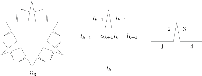
Figure 1. Three figures concerning Example 4.7: domain $\Omega_{3}$ (left), construction at level $k+1$ (middle) and enumeration of the segments (right).

Next we define $\rho(z)=d(z)^{-1/2}$ for all $z\in\Omega$ and consider the set $A=\{x\in\Sigma\,:\,a(x)\in\{2,3\}^{\mathbb{N}}\}$. It is easy to see that there are numbers $0<D_{1}<D_{2}<\infty$, so that $\dim_{d}(A)=D_{1}=\operatorname{Dim}_{d}(A)$ and $\dim_{d}(\partial\Omega_{d})=D_{2}=\operatorname{Dim}_{d}(\partial\Omega_{d})$ (actually $D_{1}=1$ and $D_{2}=2$ but this is not essential). If we show that

(4.10) $$\dim_{\rho}(A)=\operatorname{Dim}_{\rho}(A)=D_{1}/s,$$

then it follows that the claims (3) and (4) of Lemma 4.1 do not hold. Observe that $i^{-}(x)=i^{+}(x)=-1/2$ for all $x\in\partial\Omega_{d}$.

Let $x\in A$ and $y\in\overline{\Omega}_{d}$ and choose the smallest $k\in\mathbb{N}$ so that $l_{k}<2d(x,y)$. Let $z$ be as in Figure 2, i.e. $z$ is the “base point” of a cone of $\Omega_{k}$ with “side-length” $l_{k}$ which is closest to $x$. Then

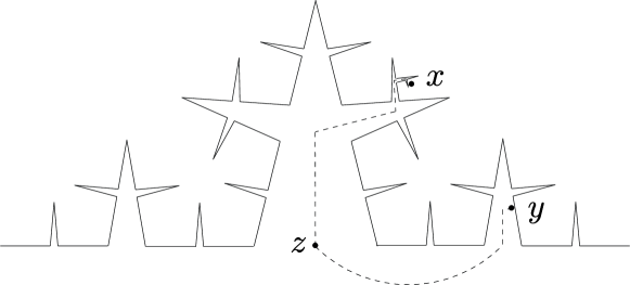
Figure 2. Selection of the“base point” $z$ in Example 4.7.

$$d_{\rho}(x,z)\leq c_{0}\sum_{n=k}^{\infty}\alpha_{n}^{-1/2}l_{n}^{1/2}=c_{0}\sum_{n=k}^{\infty}l_{n-1}^{s}\leq c_{1}l_{k}^{s}\leq 2^{s}c_{1}d(x,y)^{s}.$$

Here the first equality follows from (4.9) and the former estimate holds because $l_{k}/4<l_{k+1}<l_{k}/2$ for all $k\in\mathbb{N}$. By a similar argument, it follows that $d_{\rho}(z,y)\leq c_{2}l_{k}^{s}\leq c_{3}d(x,y)^{s}$. Thus $d_{\rho}(x,y)\leq cd(x,y)^{s}$. On the other hand, it is clear that $d_{\rho}(x,y)\geq c_{4}l_{k}^{s}\geq c^{\prime}d(x,y)^{s}$, since $a(x)\in\{2,3\}^{\mathbb{N}}$. Thus, we have $c^{\prime}d_{\rho}(x,y)\leq d(x,y)^{s}\leq cd_{\rho}(x,y)$, in other words $B_{\rho}(x,c^{\prime}r)\subset B_{d}(x,r^{s})\subset B_{\rho}(x,cr)$, for all $x\in A$ and $y\in\overline{\Omega}_{d}$ where the constants $0<c^{\prime},c<\infty$ are independent of the points $x$ and $y$. The claim (4.10) now follows from Lemma 3.2.

Remark 4.8.

Suppose that $A\subset\{x\in\partial_{\rho}\Omega\,:\,i^{-}(x)\geq\beta\}$ has the following accessibility property for some $1\leq\lambda<-1/\beta$: For each $x\in\partial\Omega_{d}$ there are $0<r,c<\infty$ such that for all $y\in B_{d}(x,r)\cap A$ there exists a curve $\gamma$ joining $x$ and $y$ so that $d(\gamma(t),\partial\Omega_{d})\geq c\min\{t^{\lambda},(\operatorname{\ell}(\gamma)-t)^{\lambda}\}$ for all $0<t<\operatorname{\ell}(\gamma)$. Then the proof of Lemma 4.1 with trivial modifications implies $(1+\lambda\beta)\dim_{\rho}(A)\leq\dim_{d}(A)$ and $(1+\lambda\beta)\operatorname{Dim}_{\rho}(A)\leq\operatorname{Dim}_{d}(A)$. On the other hand, if for each $x\in B\subset\{x\in\partial_{\rho}\Omega\,:\,i^{+}(x)\leq\beta\}$ there are $0<r,c<\infty$ so that for all curves $\gamma$ with $\gamma(0)=x$ we have $d(\gamma(t),\partial\Omega_{d})<ct^{\lambda}$ for $0<t<r$, then we get $(1+\lambda\beta)\dim_{\rho}(B)\geq\dim_{d}(B)$, $(1+\lambda\beta)\operatorname{Dim}_{\rho}(B)\geq\operatorname{Dim}_{d}(B)$. The previous example shows that these estimates are sharp.

5. Conformal densities

The results in the last section, are based on estimates of the quantities $i^{+}(x)$ and $i^{-}(x)$ which are defined as internal limits when $\Omega\ni y\rightarrow x\in\partial\Omega_{d}$. This causes a lack of the generality; it is quite possible that $i^{+}(x)=0$ and $i^{-}(x)=-1$ for all $x\in\partial\Omega_{d}$. (For instance, choose $\beta=-1$, $\lambda=0$ in the forthcoming Example 6.3.) However, if we have additional information on the geometry of $(\overline{\Omega}_{\rho},d_{\rho})$, then it might be enough to consider the ratios $\log\rho(y)/\log d(y)$ along some fixed curves or cones. The purpose of this section is to show that this is the case for so called conformal densities which arise naturally in connection with conformal and quasiconformal mappings and their generalisations, see [2].

A density $\rho$ on $\mathbb{B}^{n}$ is called a conformal density if there are constants $1\leq c_{0},c_{1}\leq\infty$ such that for each $x\in\mathbb{B}^{n}$ and for all $y\in B_{e}(x,d(x)/2)$ we have

(5.1) $$c_{0}^{-1}\leq\rho(y)/\rho(x)\leq c_{0},$$

and moreover,

(5.2) $$\mu_{\rho}(B_{\rho}(x,r))\leq c_{1}r^{n}$$

for all $r>0$. Here $\mu_{\rho}$ is the measure given by $\mu_{\rho}(E)=\int_{E}\rho^{n}\,d\mathcal{L}^{n}$ for $E\subset\mathbb{B}^{n}$. In the literature, (5.1) is often called the Harnack inequality, and one refers to (5.2) as a volume growth condition. An important corollary of the conditions (5.1)–(5.2) is the following Gehring-Hayman type estimate: There exists $1\leq c<\infty$ such that

(5.3) $$c^{-1}d_{\rho}(x,y)\leq\int_{t=0}^{d(x,y)}\rho\left((1-t)x\right)\,dt+\int_{t=0}^{d(x,y)}\rho\left((1-t)y\right)\,dt\leq cd_{\rho}(x,y)$$

for all $x,y\in\partial_{\rho}\mathbb{B}^{n}$. See [2, Theorem 3.1] and also [6].

Motivated by this estimate, we consider variants $k^{-}$ and $k^{+}$ of the quantities $i^{-}$ and $i^{+}$ for a density $\rho$ on $\mathbb{B}^{n}$ at $x\in S^{n-1}$. Recall that $k^{-}(x)=\liminf_{r\uparrow 1}\log\rho(rx)/\log(1-r)$, and $k^{+}(x)=\limsup_{r\uparrow 1}\log\rho(rx)/\log(1-r)$. Occasionally we also use $k^{-}$ and $k^{+}$ when $\Omega=\mathbb{H}$ is an open half space and then the limits are considered along straight lines orthogonal to the boundary of $\mathbb{H}$. The reduction to $k^{\pm}$ is possible since (5.3) is a much stronger condition than the Assumption 2.2 that was used earlier for the same purpose.

In the following result we only assume that (5.1) and (5.3) hold. Thus, the result applies to a slightly larger collection of densities than the conformal densities. See [12], and also Example 6.3 to follow.

Theorem 5.1.

Suppose that $\rho$ is a density on $\mathbb{B}^{n}$ that satisfies the conditions (5.1) and (5.3). Let $\beta>-1$,

$$A\subset\{x\in\partial_{\rho}\mathbb{B}^{n}\,:\,k^{+}(x)\leq\beta\},$$

$$B\subset\{x\in\partial_{\rho}\mathbb{B}^{n}\,:\,k^{-}(x)\geq\beta\},$$

$$C\subset\{x\in\partial_{\rho}\mathbb{B}^{n}\,:\,k^{-}(x)\leq\beta\}.$$

Then

1. $(1+\beta)\dim_{\rho}(A)\geq\dim_{d}(A)$,

2. $(1+\beta)\dim_{\rho}(B)\leq\dim_{d}(B)$,

3. $(1+\beta)\operatorname{Dim}_{\rho}(A)\geq\operatorname{Dim}_{d}(A)$,

4. $(1+\beta)\operatorname{Dim}_{\rho}(B)\leq\operatorname{Dim}_{d}(B)$,

5. $(1+\beta)\operatorname{Dim}_{\rho}(C)\geq\dim_{d}(C)$.

Proof.

The claims (1)–(4) have proofs very similar to the proofs of the corresponding statements of Lemma 4.1. We first apply (5.3) to conclude that for each $x\in A$ and $y\in\mathbb{B}^{n}\setminus B_{d}(x,r)$, we have

$$d_{\rho}(x,y)\geq c^{-1}\int_{t=0}^{r}\rho((1-t)x)\,dt\geq c^{-1}\int_{t=0}^{r}t^{s}\geq c_{0}r^{1+s}$$

if $s>\beta$ and $r>0$ is small. This implies $\operatorname{diam}_{d}(B_{\rho}(x,r))\leq c_{1}r^{1/(1+s)}$ and the claims (1) and (3) now follow by Lemma 3.2 (2).

To prove (2) and (4), let $s<\beta$ and for $n\in\mathbb{N}$, denote

$$B_{n}=\{x\in B\,:\,\rho((1-t)x)<t^{s}\text{ for all }0<t<1/n\}.$$

Using (5.3), we find $r_{0}>0$ so that

$$d_{\rho}(x,y)\leq c_{2}\int_{t=0}^{d(x,y)}t^{s}\leq c_{3}d(x,y)^{1+s}$$

whenever $x,y\in B_{n}$ and $d(x,y)<r_{0}$. In other words, $\operatorname{diam}_{\rho}(B_{d}(x,r)\cap B_{n})\leq c_{4}r^{1+s}$ when $0<r<r_{0}^{1/(1+s)}$. Now the Lemma 3.2 (1) implies $(1+s)\dim_{\rho}(B_{n})\leq\dim_{d}(B_{n})$ and $(1+s)\operatorname{Dim}_{\rho}(B_{n})\leq\operatorname{Dim}_{d}(B_{n})$. Note that it is enough to assume $\liminf_{r\downarrow 0}(\log\left(\operatorname{diam}_{\rho}(B_{d}(x,r)\cap A)\right))/(\log r)\geq\delta$ in Lemma 3.2 (1) (since $\dim_{\partial_{\rho}\mathbb{B}^{n}}(A)=\dim_{(A,d_{\rho})}(A)$ and $\operatorname{Dim}_{\partial_{\rho}\mathbb{B}^{n}}(A)=\operatorname{Dim}_{(A,d_{\rho})}(A)$). The claims (2) and (4) now follow since $B=\cup_{n\in\mathbb{N}}$ and $s<\beta$ is arbitrary.

It remains to prove (5). Let $x\in C$ and $s>\beta$. Then there is a sequence $0<r_{i}\downarrow 0$ such that $\rho((1-r_{i})x)>r_{i}^{s}$ for all $i$. Combined with (5.1), this gives

$$\int_{t=0}^{r_{i}}\varrho((1-t)x)\,dt\geq c_{5}r_{i}^{1+s}$$

and using also (5.3), $\operatorname{diam}_{d}(B_{\rho}(x,c_{6}r_{i}^{1+s}))\leq r_{i}$. Thus

$$\limsup_{r\downarrow 0}\frac{\log\operatorname{diam}_{d}(B_{\rho}(x,r))}{\log r}\geq\frac{1}{1+s}$$

and (5) follows from Lemma 3.2 (4). ∎

Remarks 5.2.

a) Using the claims (1)–(4) of Theorem 5.1 one may derive multifractal type formulas completely analogous to (4.4)–(4.7). Using (5), we have moreover, that $\operatorname{Dim}_{\rho}(\partial_{\rho}B_{d}(0,1))\geq\sup_{\beta>-1}\frac{e^{-}(\beta)}{1+\beta}$ where

(5.4) $$e^{-}(\beta)=\dim_{d}(\{x\in\partial_{\rho}B_{d}(0,1)\,:\,k^{-}(x)\leq\beta\}).$$

Example 6.2 shows that this is sharp in the sense that one can not replace $\dim_{d}$ by $\operatorname{Dim}_{d}$ in defining $e^{-}(\beta)$ even if $\rho$ is a conformal density.
b) We formulated the above result for densities defined on $\mathbb{B}^{n}$. The same proof goes through for any John domain $\Omega\subset\mathbb{R}^{n}$ if the condition (5.3) is replaced by

$$c^{-1}d_{\rho}(x,y)\leq\int_{t=0}^{d(x,y)}\rho(\gamma_{x}(t))\,dt+\int_{t=0}^{d(x,y)}\rho(\gamma_{y}(t))\,dt\leq cd_{\rho}(x,y),$$

where $\gamma_{x}$ is a fixed $\alpha$-cone with $\gamma_{x}(0)=x$ for each $x\in\partial_{\rho}\Omega$. Actually, we could even weaken this in the spirit of (2.2) and assume only that for all $\varepsilon>0$, we have

$$d_{\rho}(x,y)^{1+\varepsilon}\leq\int_{t=0}^{d(x,y)}\rho(\gamma_{x}(t))\,dt+\int_{t=0}^{d(x,y)}\rho(\gamma_{y}(t))\,dt\leq d_{\rho}(x,y)^{1-\varepsilon}$$

when $d(x,y)$ is small enough.
c) Makarov [9, Theorems 0.5, 0.6] proved results essentially similar to Theorem 5.1 (1)–(2) in case $\beta>0$ and $\rho=|f^{\prime}|$ for $f$ conformal. He also showed [9, Theorem 0.8] that $k^{-}$ cannot be replaced by $k^{+}$ in (2).
d) In [2], Bonk, Koskela, and Rohde proved the following deep fact. If $\rho$ is a conformal density on $\mathbb{B}^{n}$, then:

(5.5) $$\text{There is }E\subset S^{n-1}\text{ with }\dim_{d}E=0\text{ such that }\dim_{\rho}(\partial_{\rho}\mathbb{B}^{n}\setminus E)\leq n.$$

See [2, Theorem 7.2]. As a central tool, they used an estimate analogous to Theorem 5.1 (2). In fact, combining Theorem 5.1 (2) and [2, Theorem 5.2] gives a simpler proof for (5.5) than the one given in [2]. However, their result is quantitatively stronger than (5.5).
e) A generic situation in which Theorem 5.1 is stronger than Theorem 4.2 will be discussed in Example 6.3.

6. Further examples, remarks, and questions

We first give the example mentioned in Remark 5.2 e) showing that one can not replace $\dim_{d}$ by $\operatorname{Dim}_{d}$ in defining $e^{-}(\beta)$. We will make use of the following lemma. We formulate it in a more general setting, for future reference.

Lemma 6.1.

Let $\Omega\subset\mathbb{R}^{n}$ be a $(2\alpha)$-John domain and $C\subset\partial\Omega_{d}$. Suppose that $\widetilde{\rho}\colon(0,\infty)\rightarrow(0,\infty)$ is nonincreasing and and satisfies $\int_{0}^{1}\widetilde{\rho}(t)dt<\infty$. Define $\rho(x)=\widetilde{\rho}(d(x,C))$ for $x\in\Omega$. Then for all $x\in C$ and $0<r<\operatorname{diam}_{d}(\Omega)/2$, it holds

(6.1) $$\operatorname{diam}_{d}\left(B_{\rho}\left(x,\frac{1}{2}\int_{t=0}^{r}\widetilde{\rho}(t)dt\right)\right)\leq 2r,$$

(6.2) $$\operatorname{diam}_{\rho}\left(B_{d}(x,r)\right)\leq c_{1}\int_{t=0}^{c_{2}r}\widetilde{\rho}(t)\,dt$$

for some constants $0<c_{1},c_{2}<\infty$ that depend only on $\alpha$ and $n$.

Proof.

Let $x\in C$ and $y\in\overline{\Omega}_{d}$. Denote $d=d(x,y)$ and suppose that $\gamma$ is a curve joining $x$ and $y$. To prove (6.1), it suffices to show that

(6.3) $$\operatorname{\ell}_{\rho}(\gamma)\geq\frac{1}{2}\int_{t=0}^{d}\widetilde{\rho}(t)\,dt.$$

Let $h=h(\gamma)=\max_{0\leq t\leq L}d(\gamma(t))$ where $L=\operatorname{\ell}(\gamma)$. Then $\operatorname{\ell}_{\rho}(\gamma)\geq\tfrac{1}{2}\int_{t=0}^{h}\widetilde{\rho}(t)\,dt+\tfrac{1}{2}d\rho(h)$. If $h\geq d$ the estimate (6.3) clearly holds. If $h<d$, then $d\widetilde{\rho}(h)\geq\int_{t=h}^{d}\widetilde{\rho}(t)dt$ since $\widetilde{\rho}$ is nonincreasing and consequently

$$\operatorname{\ell}_{\rho}(\gamma)\geq\frac{1}{2}\left(\int_{r=0}^{h}\widetilde{\rho}(r)\,dr+d\widetilde{\rho}(h)\right)\geq\frac{1}{2}\int_{t=0}^{d}\widetilde{\rho}(t)\,dt.$$

This settles the proof of (6.1).

To prove (6.2), let $x\in C$ and $r>0$. We use Lemma 3.3 to cover $B_{d}(x,r)$ with sets $B_{\alpha}(x_{i},cr)$, $i=1,\ldots,N=N(n,\alpha)$. Let $y\in B_{\alpha}(x_{i},cr)$ and pick an $\alpha$-cigar $\gamma$ with $\operatorname{\ell}(\gamma)\leq cr$ joining $y$ to $x_{i}$. Now

(6.4) $$d_{\rho}(y,x_{i})\leq\int_{\gamma}\widetilde{\rho}(d(z,C))|dz|\leq 2\int_{t=0}^{cr/2}\widetilde{\rho}(\alpha t)\,dt=\frac{2}{\alpha}\int_{t=0}^{\alpha cr/2}\widetilde{\rho}(t)\,dt.$$

As $B_{d}(x,r)$ is (path-)connected and is covered by $N$ sets of the type $B_{\alpha}(x_{i},cr_{i})$, we arrive at $\operatorname{diam}_{\rho}(B_{d}(x,r))\leq(4N/\alpha)\int_{t=0}^{\alpha cr/2}\widetilde{\rho}(t)\,dt$ proving the claim. ∎

Example 6.2.

We show that $\dim_{d}$ cannot be replaced by $\operatorname{Dim}_{d}$ in (5.4) even if $\rho$ is a conformal density.

We first fix numbers $0<a<b<1/2$, $-1<\lambda<\eta<0$, and $\xi$ such that

(6.5) $$a^{1+\lambda}=b^{1+\eta}=\xi,$$

and

(6.6) $$-\log 2<\log\xi<-\tfrac{1}{2}\log 2.$$

Let us also pick natural numbers $n_{1}<N_{1}<n_{2}<N_{2}<n_{3}<N_{3}<\ldots$. We let $C\subset S^{1}$ denote a Cantor set constructed as follows (See the construction in Example 4.6). We start with an arc of length $1$ and remove an arc of length $1-2a$ from the middle. Next, we remove arcs of length $a(1-2a)$ from the middle of the two remaining arcs. We iterate this construction for $n_{1}$ steps. After these $n_{1}$ steps, we have $2^{n_{1}}$ arcs of length $a^{n_{1}}$. At the step $n_{1}+1$, we remove arcs of relative length $1-2b$ from the middle of each of these arcs. We continue the construction with the parameter $b$ for $N_{1}-n_{1}$ steps. Then we use again the parameter $a$ for $n_{2}-N_{1}$ steps and so on. We denote by $E_{k,1}\ldots,E_{k,2^{k}}$ the arcs remaining after $k$ steps and denote by $\ell_{k}$ the length of these arcs. What remains at the end is the Cantor set $C=\cap_{k\in\mathbb{N}}\cup_{i=1}^{2^{k}}E_{k,i}$.

Let $r_{0}=R_{1}=1$, $r_{1}=\ell_{n_{1}}=a^{n_{1}}$, $R_{2}=\ell_{N_{1}}=a^{n_{1}}b^{N_{1}-n_{1}}$, $r_{2}=\ell_{n_{2}}=a^{n_{1}+n_{2}-N_{1}}b^{N_{1}-n_{1}}$ and so on. Thus $r_{i}$ (resp. $R_{i}$) is the length of a construction interval of $C$ of level $n_{i}$ (resp. $N_{i-1}$). We define $\rho(x)=\widetilde{\rho}(\operatorname{dist}(x,C))$ for all $x\in\mathbb{B}^{2}$, where $\widetilde{\rho}$ is the function defined by

$$\widetilde{\rho}(t)=\begin{cases}\left(\frac{R_{1}R_{2}\cdots R_{k}}{r_{0}r_{1}\cdots r_{k-1}}\right)^{\eta-\lambda}t^{\lambda},\quad r_{k}\leq t\leq R_{k},\\ \left(\frac{R_{1}R_{2}\cdots R_{k}}{r_{0}r_{1}\cdots r_{k}}\right)^{\eta-\lambda}t^{\eta},\quad R_{k+1}\leq t\leq r_{k}.\end{cases}$$

Now, if $N_{i}/n_{i},n_{i+1}/N_{i}\rightarrow\infty$ fast enough, it is easy to see that $\dim_{d}C=-\log 2/\log a$ and $\operatorname{Dim}_{d}C=-\log 2/\log b$, see e.g. [10, p. 77]. Moreover, it then follows that $k^{-}(x)=\lambda$ if $x\in C$ and $k^{-}(x)=0$ otherwise. Next, let $h_{k}=\int_{t=0}^{\ell_{k}}\widetilde{\rho}(t)\,dt$. Since

(6.7) $$\widetilde{\rho}(\ell_{k})\ell_{k}=\xi^{k}$$

for all $k$ (combine (6.5) with the definitions), it follows that

$$\tfrac{1}{2}\xi^{k}=\tfrac{1}{2}\widetilde{\rho}(\ell_{k})\ell_{k}\leq\int_{t=\ell_{k+1}}^{\ell_{k}}\widetilde{\rho}(t)\leq\widetilde{\rho}(\ell_{k+1})\ell_{k}\leq a^{\lambda}\widetilde{\rho}(\ell_{k})\ell_{k}=a^{\lambda}\xi^{k}.$$

Thus

(6.8) $$\tfrac{1}{2}\xi^{k}\leq h_{k}=\sum_{m\geq k}\int_{t=\ell_{m+1}}^{\ell_{m}}\widetilde{\rho}(t)\,dt\leq c_{0}\xi^{k}.$$

From Lemma 6.1, it follows that for each $I=I_{k,i}$ we have

(6.9) $$c_{1}h_{k}\leq\operatorname{diam}_{\rho}(I)\leq c_{2}h_{k}$$

for some constants $0<c_{1}<c_{2}<\infty$. Let $\mu$ be the natural probability measure on $C$ that satisfies $\mu(I_{k,i})=2^{-k}$. Then

$$\lim_{k\rightarrow\infty}\frac{\log\mu(I_{k,i})}{\log(\operatorname{diam}_{\rho}(I_{k,i}))}=\frac{-\log 2}{(1+\lambda)\log a},$$

using (6.8) and (6.9). But this implies $\dim_{\rho}(C)=\operatorname{Dim}_{\rho}(C)=(-\log 2)/((1+\lambda)\log a)$, see e.g. [4, Proposition 10.1] and [3, Corollary 3.20]. Thus,

$$1<\operatorname{Dim}_{\rho}(C) =\operatorname{Dim}_{\rho}(S^{1})=\frac{-\log 2}{(1+\lambda)\log a}<\frac{-\log 2}{(1+\lambda)\log b}=\frac{\operatorname{Dim}_{d}(C)}{1+\lambda}$$

$$=\sup_{\beta>-1}\frac{\operatorname{Dim}_{d}(\{x\in\partial_{\rho}B_{d}(0,1)\,:\,k^{-}(x)\leq\beta\}}{1+\beta}\,,$$

recall (6.6).

It remains to prove that $\rho$ is a conformal density. The condition (5.1) is clearly satisfied so we only have to verify (5.2). We show this for $x\in C$ and $0<r<1$ (the general case $x\in\mathbb{B}^{2}$ follows easily from this). Using (5.1) we may also assume that $r=h_{k}$ for some $k\in\mathbb{N}$. For each $m\geq k$, we denote

$$A_{m}=\{y\in B_{d}(x,c_{3}\ell_{k})\,:\,\ell_{m}\leq d(y,C)\leq c_{3}\ell_{m}\}.$$

Then $B_{\rho}(x,h_{k})\subset\cup_{m\geq k}A_{m}$, for a suitable constant $1<c_{3}<\infty$, recall (6.9). Moreover, it follows from (5.1) and (6.7) that $c_{4}\xi^{m}/\ell_{m}\leq\rho(y)\leq c_{5}\xi^{m}/\ell_{m}$ for all $y\in A_{m}$, where $0<c_{4}<c_{5}<\infty$ depend only on $a,b,\lambda$, and $\eta$. Since $\mathcal{L}^{2}(A_{m})\leq c_{6}2^{m-k}\ell_{m}^{2}$, we arrive at

$$\mu_{\rho}(A_{m})=\int_{A_{m}}\rho^{2}\,d\mathcal{L}^{2}\leq c_{7}2^{m-k}\xi^{2m}.$$

As $2\xi^{2}<1$ by (6.6), this yields

$$\mu_{\rho}(B_{\rho}(x,h_{k}))\leq\sum_{m\geq k}\mu_{\rho}(A_{m})\leq c_{7}\sum_{m\geq k}2^{m-k}\xi^{2m}\leq c_{8}\xi^{2k}\leq c_{9}h_{k}^{2},$$

where the last estimate follows from (6.8).

Below, we construct a “multifractal type” example and calculate the Hausdorff dimension of the boundary using Theorem 5.1.

Example 6.3.

We construct a domain and a conformal density that satisfies Gehring-Hayman condition (5.3) and compute the Hausdorff dimension of the boundary.

We define a density $\rho$ on the upper half-plane $H\subset\mathbb{R}^{2}$ (actually we define $\rho(z)$ only for $z\in[0,1]\times(0,3]$ but the definition is easily extended to the whole of $H$). Let $-1<\beta,\lambda<0$, $\beta\neq\lambda$. We consider the triadic decomposition of $[0,1]$; Let $I_{\varnothing}=[0,1]$, $I_{0}=[0,1/3]$, $I_{1}=[1/3,2/3]$, and $I_{2}=[2/3,1]$. If $n\in\mathbb{N}$ and, $\textbf{i}\in\{0,1,2\}^{n}$, let $I_{\textbf{i}0},I_{\textbf{i}1},I_{\textbf{i}2}$ denote its triadic subintervals enumerated from left to right. For each such triadic interval $I=I_{\textbf{i}}$, let $Q_{\textbf{i}}=I\times\left[|I|,3|I|\right]$. Next we define weights $\rho_{\textbf{i}}$ inductively by the rules $\rho_{\varnothing}=1$ and $\rho_{\textbf{i}0}=\rho_{\textbf{i}2}=3^{-\lambda}\rho_{\textbf{i}}$, $\rho_{\textbf{i}1}=3^{-\beta}\rho_{\textbf{i}}$.

Let $\rho\colon[0,1]\times(0,3]\rightarrow(0,\infty)$ be a density such that $\rho(x_{\textbf{i}})=\rho_{\textbf{i}}$ if $x_{\textbf{i}}$ is the centre point of $Q_{\textbf{i}}$. We also require that the condition (5.1) holds with some $c_{0}<\infty$. This is possible because of the symmetric definition of $\rho_{\textbf{i}}$: If $I_{\textbf{i}}$ and $I_{\textbf{j}}$ are neighbouring intervals of the same length, then $3^{-|\beta-\lambda|}\leq|\rho_{\textbf{i}}/\rho_{\textbf{j}}|\leq 3^{|\beta-\lambda|}$.

We will next show that the Gehring-Hayman condition (5.3) holds for the density $\rho$. Let $x,y\in[0,1]$ with $y-x=r>0$. Let $\gamma_{1}$, $\gamma_{2}$, and $\gamma_{3}$ be the line segments joining $(x,0)$ to $(x,r)$, $(x,r)$ to $(y,r)$, and $(y,r)$ to $(y,0)$, respectively. Then a direct calculation using the definitions gives

$$\int_{\gamma_{1}}\rho(z)\,|dz|\leq c_{1}\int_{t=0}^{r}t^{\min\{\beta,\lambda\}}\frac{\rho(x,r)}{r^{\min\{\beta,\lambda\}}}\,dt\leq c_{2}r\rho(x,r),$$

$$\int_{\gamma_{3}}\rho(z)\,|dz|\leq c_{1}\int_{t=0}^{r}t^{\min\{\beta,\lambda\}}\frac{\rho(y,r)}{r^{\min\{\beta,\lambda\}}}\,dt\leq c_{2}r\rho(y,r).$$

Combining these estimates with (5.1), we obtain

(6.10) $$c_{3}\operatorname{\ell}_{\rho}(\gamma_{i})\leq\operatorname{\ell}_{\rho}(\gamma_{2})\leq c_{4}\operatorname{\ell}_{\rho}(\gamma_{i})$$

for $i=1,3$. The condition (5.3) is satisfied if we can show that $\operatorname{\ell}_{\rho}(\gamma)\geq c\operatorname{\ell}_{\rho}(\gamma_{2})$ for any curve joining $x$ and $y$ in $H$. Denote $h=h(\gamma)=\max_{0<t<\operatorname{\ell}(\gamma)}d(\gamma(t))$. If $h\leq r$, it follows that $\operatorname{\ell}_{\rho}(\gamma)\geq c\operatorname{\ell}_{\rho}(\gamma_{2})$ since $\rho$ is essentially decreasing on each vertical line segment. More precisely using (5.3) and the definitions of the weights $\rho_{\textbf{i}}$, we get

(6.11) $$\rho(a,tb)\geq c_{5}\rho(a,b)$$

if $(a,b)\in[0,1]\times(0,3]$ and $0<t<1$. Now suppose that $h>r$ and let $z=\gamma(t_{0})$ where $t_{0}=\min\{t>0\,:\,d(\gamma(t))=r\}$. If $d(z,\gamma_{2})<r$, it follows easily from (5.1) that $\operatorname{\ell}_{\rho}(\gamma)\geq c\operatorname{\ell}_{\rho}(\gamma_{2})$. If $d(z,\gamma_{2})\geq r$, let $\eta$ be the line segment joining $z$ to the closest point of $\gamma_{2}$. Then (6.11) implies $\operatorname{\ell}_{\rho}(\gamma)\geq c_{5}\operatorname{\ell}_{\rho}(\eta)\geq c\operatorname{\ell}_{\rho}(\gamma_{2})$ where the last estimate follows using (5.1). This settles the proof of (5.3).

We will next compute the Hausdorff dimension of the boundary. Let $0\leq t\leq 1$ and denote $A_{t}=\{x\in[0,1]\,:\,k^{-}(x)=k^{+}(x)=t\beta+(1-t)\lambda\}$. Then

$$A_{t} =\left\{x=\sum_{i\in\mathbb{N}}x_{i}3^{-i}\,:\,x_{i}\in\{0,1,2\}\text{ and }\lim_{n\rightarrow\infty}\#\{1\leq i\leq n\,:\,x_{i}=1\}/n=t\}\right\}.$$

Using this expression, we get

(6.12) $$\dim_{d}(A_{t})=\operatorname{Dim}_{d}(A_{t})=\frac{-t\log t+(t-1)\log((1-t)/2)}{\log 3}.$$

Indeed, if $\mu_{t}$ is the unique Borel probability measure on $[0,1]$ that satisfies $\mu_{t}(I_{\textbf{i}1})=t\mu_{t}(I_{\textbf{i}})$ and $\mu_{t}(I_{\textbf{i}0})=\mu_{t}(I_{\textbf{i}2})$ for all triadic intervals $I_{\textbf{i}}$, then we have

$$\lim_{r\downarrow 0}\frac{\log\mu_{t}((B_{d}(x,r))}{\log r}=\frac{-t\log t+(t-1)\log((1-t)/2))}{\log 3}$$

and this implies (6.12). For instance, see [4, Proposition 10.4].

Thus, from Theorem 5.1 and (6.12), we get

(6.13) $$\dim_{\rho}(A_{t})=\operatorname{Dim}_{\rho}(A_{t})=\frac{-t\log t+(t-1)\log((1-t)/2)}{(1+t\beta+(1-t)\lambda)\log 3}\,.$$

If $f(\beta,\lambda)$ is the maximum of (6.13) over all $0\leq t\leq 1$, then we conclude that

$$\operatorname{Dim}_{\rho}(\partial_{\rho}H)\geq\dim_{\rho}(\partial_{\rho}H)\geq f(\beta,\lambda).$$

To finish this example, we show that for the Hausdorff dimension, there is an equality in the above estimate. We give the proof in the case $\beta<\lambda$, the case $\lambda<\beta$ can be handled with similar arguments. First, we observe using Theorem 5.1 (2) that

$$\dim_{\rho}(\{k^{-}(x)\geq\beta/3+2\lambda/3\})\leq 1/(1+\beta/3+2\lambda/3)<f(\beta,\lambda),$$

where the strict inequality is obtained via differentiating (6.13) at $t=1/3$. On the other hand, if $t>1/3$, and $A^{-}_{t}=\{x\in[0,1]\,:\,k^{-}(x)\leq t\beta+(1-t)\lambda\}$, then

$$A^{-}_{t}=\{x=\sum_{i\in\mathbb{N}}x_{i}3^{-i}\,:\,\limsup_{n\rightarrow\infty}\#\{1\leq i\leq n\,:\,x_{i}=1\}/n\geq t\}\}$$

and thus $\dim_{d}(A^{-}_{t})\leq(-t\log t+(t-1)\log((1-t)/2))/\log 3$. To see this, observe that

$$\liminf_{r\downarrow 0}\frac{\log\mu_{t}(B_{d}(x,r))}{\log r}\leq\frac{-t\log t+(t-1)\log((1-t)/2))}{\log 3}$$

for all $x\in A^{-}_{t}$ and use [4, Proposition 10.1]. Now, using the analogue of (4.6) for $k^{-}$ implies $\dim_{\rho}(\partial_{\rho}H)\leq f(\beta,\lambda)$, and consequently $\dim_{\rho}(\partial_{\rho}H)=f(\beta,\lambda)$.

Remarks 6.4.

a) One can estimate the numbers $f(\beta,\lambda)$ numerically. For instance, if $\beta=-1/2$ and $\lambda=-1/3$, then $f(\beta,\lambda)\approx 1.65$.
b) Inspecting (6.13), it is easy to see that

$$\max\{1/(1+\beta/3+2\lambda/3),\log 2/((1+\lambda)\log 3)\}<f(\beta,\lambda)<1/(1+\min\{\beta,\lambda\})$$

for all choices of $\beta$ and $\lambda$.
c) If above $\beta,\lambda>-1/2$, then it is not hard to see that $\rho$ satisfies (5.2) and thus is a conformal density.

We do not know if also $\operatorname{Dim}_{\rho}(\partial_{\rho}H)\leq f(\beta,\lambda)$:

Question 6.5.

In Example 6.3, is it true that $\operatorname{Dim}_{\rho}(\partial_{\rho}H)=f(\beta,\lambda)$?

We cannot use Theorem 5.1 to solve this question since it can be shown that $\operatorname{Dim}_{d}(\{x\,:k^{-}(x)=\min\{\beta,\lambda\})=1$.

It is true that $\dim_{\rho}(\partial_{\rho}\mathbb{B}^{n})\geq n-1$ for all conformal densities $\rho$ defined on $\mathbb{B}^{n}$. This deep fact was proved in [1]. A straightforward estimate using Theorem 5.1 and (5.1) only implies that $\dim_{\rho}(\partial_{\rho}\mathbb{B}^{n})\geq c(n,c_{0})>0$, where $c_{0}$ is the constant in (5.1). See also [2, Proposition 7.1]. Next we provide an example of a density $\rho$ on the upper half-plane $H$ such that $\operatorname{Dim}_{\rho}(\partial_{\rho}H)=0$ and $\dim_{d}(\mathbb{R}\setminus\partial_{\rho}H)=0$.

Example 6.6.

We construct a density with $\operatorname{Dim}_{\rho}(\partial_{\rho}H)=0$ and $\dim_{d}(\mathbb{R}\setminus\partial_{\rho}H)=0$.

Given an interval $I\subset\mathbb{R}$, let $T_{I}$ and $U_{I}$ be the isosceles triangles with base $I$ and heights $|I|$ and $|I|/2$ respectively. Denote $S_{I}=T_{I}\setminus U_{I}$.

To begin with, let $I_{1},I_{2},\ldots$ be disjoint intervals so that $C=\mathbb{R}\setminus\cup I_{i}$ forms a Cantor set (a nowhere dense closed set without isolated points). Moreover, we assume that $\sum_{i}\operatorname{diam}_{d}(I_{i})\leq 1$. Let $\rho(x)=\exp(-1/d(x))$ if $x\in H\setminus\cup_{i}T_{I_{i}}$. We define $\rho$ on each strip $S_{I_{i}}$ so that

(6.14) $$\ell_{\rho}(\gamma)\geq 1$$

for any curve joining $U_{I_{i}}$ to $H\setminus T_{I_{i}}$. We also require that $\rho$ extends continuously to the lower boundary $\Gamma_{I_{i}}$ of $S_{I_{i}}$ (excluding the two endpoints of $I_{i}$) and that

(6.15) $$\ell_{\rho}(\gamma)=\infty$$

if $\gamma$ is a curve on $S_{I_{i}}$ whose one endpoint is an endpoint of $I_{i}$. We remark that the condition (6.15) as well as the condition (6.17) below, are only used to ensure that the assumption (A2) is satisfied.

Now for each $x,y\in C$ with $d(x,y)=d>0$, we have

$$d_{\rho}(x,y)\leq 2\int_{t=0}^{d}\exp(-1/t)\,dt+d\exp(-1/d)\leq 3\exp(-1/d).$$

Thus, for each $n\in\mathbb{N}$, there is $\delta>0$ such that $d_{\rho}(x,y)\leq d(x,y)^{n}$ if $x,y\in C$ and $d(x,y)<\delta$. By Lemma 3.1, this implies $\operatorname{Dim}_{\rho}(C)=0$.

We continue the construction inside the triangles $U_{I_{i}}$. We choose intervals $I_{i,j}\subset I_{i}$ so that $C_{i}=I_{i}\setminus\cup_{j}I_{i,j}$ is a Cantor set and

(6.16) $$\sum_{i,j}\operatorname{diam}_{d}(I_{i,j})^{1/2}\leq 1.$$

We define $\rho(x)=f_{i}(x)\exp(-1/d(x))$ on $U_{i}\setminus\cup_{j}T_{I_{i,j}}$ where $f_{i}(x)$ is a continuous weight that is bounded if $x$ is bounded away from the endpoints of $I_{i}$. Close to the endpoints of $I_{i}$, we make $f_{i}$ so large that

(6.17) $$\ell_{\rho}(\gamma)=\infty$$

if $\gamma$ is a curve on $U_{I_{i}}$ whose one endpoint is an endpoint of $I_{i}$. Also, we define $\rho$ on the strips $S_{I_{i}}$ so that analogues of (6.14) and (6.15) hold. As above, we see that $\operatorname{Dim}_{\rho}(C_{i})=0$ for all $i$.

We continue the construction inductively inside the triangles $U_{I_{i,j}}$. At the step $n$, we obtain Cantor sets $C_{n,i}$ with $\operatorname{Dim}_{\rho}(C_{n,i})=0$. At the end, $\partial_{\rho}H$ will be the union of all these Cantor sets. Replacing the exponent $1/2$ in (6.16) by $1/n$ at the step $n$ implies that $\dim_{d}(\mathbb{R}\setminus\partial_{\rho}H)=0$.

It would be interesting to know, if the analogy of (5.5) for the packing dimension holds.

Question 6.7.

If $\rho$ is a conformal density on $\mathbb{B}^{n}$, does there exist a set $A\subset S^{n-1}$ with $\operatorname{Dim}_{d}(A)=0$ such that $\operatorname{Dim}_{\rho}(S^{n-1}\setminus A)\leq n$?

Acknowledgements. The first author was supported by the Academy of Finland project #120972 and he wishes to thank professor Pekka Koskela. The second author was supported by the Academy of Finland project #126976.

References

- [1] Mario Bonk and Pekka Koskela. Conformal metrics and size of the boundary. Amer. J. Math., 124(6):1247–1287, 2002.
- [2] Mario Bonk, Pekka Koskela, and Steffen Rohde. Conformal metrics on the unit ball in Euclidean space. Proc. London Math. Soc., 77(3):635–664, 1998.
- [3] Colleen D. Cutler. The density theorem and Hausdorff inequality for packing measure in general metric spaces. Illinois J. Math., 39(4):676–694, 1995.
- [4] Kenneth Falconer. Techniques in fractal geometry. John Wiley & Sons Ltd., Chichester, 1997.
- [5] John B. Garnett and Donald E. Marshall. Harmonic measure, volume 2 of New Mathematical Monographs. Cambridge University Press, Cambridge, 2005.
- [6] F. W. Gehring and W. K. Hayman. An inequality in the theory of conformal mapping. J. Math. Pures Appl. (9), 41:353–361, 1962.
- [7] C. Kenig, D. Preiss, and T. Toro. Boundary structure and size in terms of interior and exterior harmonic measures in higher dimensions. J. Amer. Math. Soc., 22(3):771–796, 2009.
- [8] N. G. Makarov. On the distortion of boundary sets under conformal mappings. Proc. London Math. Soc. (3), 51(2):369–384, 1985.
- [9] N. G. Makarov. Conformal mapping and Hausdorff measures. Ark. Mat., 25(1):41–89, 1987.
- [10] Pertti Mattila. Geometry of Sets and Measures in Euclidean Spaces: Fractals and rectifiability. Cambridge University Press, Cambridge, 1995.
- [11] Tomi Nieminen. Conformal metrics and boundary accessibility. Illinois J. Math., 53(1):25–38, 2009.
- [12] Tomi Nieminen and Timo Tossavainen. Conformal metrics on the unit ball: the Gehring-Hayman property and the volume growth. Conform. Geom. Dyn., 13:225–231, 2009.
- [13] Ch. Pommerenke. Boundary behaviour of conformal maps, volume 299 of Grundlehren der Mathematischen Wissenschaften [Fundamental Principles of Mathematical Sciences]. Springer-Verlag, Berlin, 1992.