Quasi-deterministic transport of Brownian particles in an oscillating periodic potential

Abstract

We consider overdamped Brownian dynamics in a periodic potential with temporally oscillating amplitude. We analyze the transport which shows effective diffusion enhanced by the oscillations and derive approximate expressions for the diffusion coefficient. Furthermore we analyze the effect of the oscillating potential on the transport if additionally a constant force is applied. We show the existence of synchronization regimes at which the deterministic dynamics is in resonance with the potential oscillations giving rise to transport with extremely low dispersion. We distinguish slow and fast oscillatory driving and give analytical expressions for the mean velocity and effective diffusion.

In recent decades there has been intense research on transport phenomena in Brownian dynamics. Numerous publications analyze the diffusive transport in spatially periodic potentials and report interesting behavior of the diffusion coefficient Reimann et al. (2001); Lindenberg (2007); borromeo_resonant_2008 . Diverse sorts of ratchets have been investigated Reimann (2002); Anishchenko et al. (2002); Hänggi and Marchesoni (2008) where particles move in periodic potentials and time dependent forces or modulations of the potential enhance a directed flow. Most of the research focused on mean drift within such systems and on the conditions under which the directed transport is maximized. Also the diffusion coefficient in these temporally changing potentials have been calculated Freund and Schimansky-Geier (1999) and it was proposed to take the diffusion coefficient to evaluate the precision of stochastic directed transport Lindner and Schimansky-Geier (2002).

In this spirit we will focus this work on overdamped Brownian transport in a temporally oscillating and spatially periodic potential. The interplay of the different time scales in the system, given by the period of the oscillating potential, the relaxation time of the deterministic dynamics and the diffusion time gives rise to non-trivial dynamical phenomena, such as an oscillation driven enhancement of the effective diffusion. Otherwise if additionally external forces are applied, the particle’s motion becomes quasi-deterministic following the oscillations in direction of the applied force jumping several periods of the potential with minimal diffusion. Experimental systems where such temporal modulations could be realized are free-flow dielectrophoresis Ajdari and Prost (1991), colloidal particles in optical fields Faucheux et al. (1995); Tatarkova et al. (2003); Bleil et al. (2007), Josephson-junctions Kautz (1996); Sterck et al. (2009) or paramagnetic colloids in magnetic fields Tierno et al. (2008); Auge et al. (2009). With small modification the dynamics can also describe neuronal activity being one type of a firing theta-neuron Ermentrout and Kopell (1986); Neiman and Russell (2005).

We consider an overdamped Brownian particle under the influence of thermal fluctuations in spatially periodic potential with harmonically oscillating amplitudes. The corresponding Langevin equation written in dimensionless form reads

$$\dot{y}=\cos(y)\sin(\Omega\tau)+F+\sqrt{2D}\,\xi(t),$$ (1)

with driving frequency $\Omega$, constant force $F$, and noise intensity $D$.

As characteristic observables we investigate the asymptotic drift velocity and the effective diffusion coefficient

$$v_{\textrm{drift}}=\lim_{\tau\to\infty}\frac{\langle y(\tau)\rangle-\langle y(0)\rangle}{\tau}$$ (2)

$$D_{\textrm{eff}}=\lim_{\tau\to\infty}\frac{1}{2}\frac{d}{d\tau}\langle(y-\langle y(\tau)\rangle)^{2}\rangle.$$ (3)

Here $\langle\cdot\rangle$ denotes the ensemble average.

In the case of non-vanishing flux in the system ($F\neq 0$) we measure the quality of the directed transport by the so called Péclet number Freund and Schimansky-Geier (1999): $\textrm{Pe}=v_{\textrm{drift}}L/D_{\textrm{eff}}$ where $L$ is the characteristic length scale of the system. Here we set $L$ equal to the spatial wave length $\lambda=2\pi$. For $\textrm{Pe}<1$ diffusion dominates the dynamics, and the directed transport plays a minor role in comparison with the non-directed spread of the probability distribution. For $\textrm{Pe}>1$ the transport is dominated by the drift. The limit of $\textrm{Pe}\to\infty$ corresponds to a deterministic transport with vanishing effective diffusion on the characteristic length scale $L$.

First we consider the case without bias in the system for $F=0$. The spatial and temporal symmetry in the potential prevents any directed flux within the system ($v_{\textrm{drift}}=0$). For large noise intensities the influence of the potential is negligible and the dynamics corresponds to a free Brownian motion with $D_{\textrm{eff}}=D$ whereas in the limit of vanishing noise the interplay of two time scales controls the dynamics. On the one hand the external driving period $T=2\pi/\Omega$ and secondly the intrinsic relaxation time $\tau_{r}$ from an unstable potential maximum to a stable minimum.

At oscillation frequencies much faster than the relaxation time $\Omega\gg 1/\tau_{r}$ the potential is self-averaged to be effectively flat for the particle dynamics and the effective diffusion also converges to the free Brownian diffusion coefficient $D$ for $\Omega\to\infty$. However, for a relaxation time shorter than the half oscillation period $\tau_{r}<T/2=\pi/\Omega$ trajectories are able to approach the next minimum until the oscillation changes the minimum into a metastable maximum. Involving a small amount of noise the particle performs effectively discrete jumps between the minima of the potential for the extreme potential settings (maximal barriers).

This behavior can be easily described by an oscillation induced random walk. The equally distributed jumps to the left and right take place at discrete time intervals $T/2$ and correspond to the switching of the fixed points (two jumps per full period). The jump length is given by $l=\lambda/2=\pi$. Thus the probability to find the particle at the position $y_{i}=i\cdot l$ after $N$ jumps is given by the binomial distribution, which converges towards a Gaussian distribution in the long time limit describing diffusion with effective coefficient $D_{\textrm{eff}}=\pi\Omega/2$. As discussed above for large frequencies the effective diffusion will reach asymptotically the noise intensity $D$. So the linear relation can not hold for the whole frequency range but has to pass a maximum.

An initial Gaussian distribution around a stable fixed point (potential minimum) $y_{n}$ splits as the fixed point becomes unstable (transforms into a potential maximum). For intermediate frequencies only a certain fraction of the particle ensembles can reach the next minimum. The remaining part moves back into the initial position. We attempt to describe this mechanism by approximating the probability $u(\Omega,D)$ of a particle starting at $y_{n}+\delta$ ($\delta\geq 0$) from which a particle is able to arrive at the neighboring fixed point $y_{\textrm{end}}=y_{n+1}-\epsilon$. Here $\epsilon$ represents a small distance which the particle overcomes by fluctuations alone. This probability is given by the complementary error function

$$u(\Omega,D)=\textrm{erfc}\left(\frac{\delta}{\sqrt{2\sigma^{2}}}\right),$$ (4)

with the width $\sigma^{2}$ as the particle distribution at $y_{n}$ and $\delta=2\,\textrm{arctan}\left[\exp\left(-2/\Omega\right)\textrm{cot}\left(\epsilon/2\right)\right]$ as the initial deviation. The new expression for the effective diffusion coefficient has to be scaled by taking Eq. 4 into account and we get

$$D_{\textrm{eff}}=\frac{\pi\Omega}{2}\textrm{erfc}\left(\sqrt{\frac{2}{\sigma^{2}}}\,\textrm{arctan}\left[e^{-\frac{2}{\Omega}}\textrm{cot}\left(\frac{\epsilon}{2}\right)\right]\right).$$ (5)

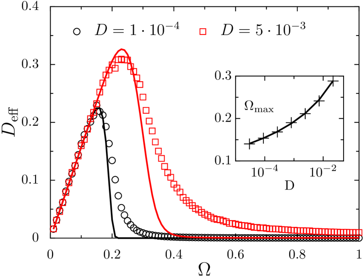
Figure 1: Effective diffusion vs. driving frequency from simulations for $F=0$ and $D=1.0\cdot 10^{-4}$ (circles), $D=5.0\cdot 10^{-3}$ (squares) in comparison with results of of Eq. 5 (solid lines) for $e=0.09$ and $b=150$. The inset shows the prediction on the the position $\Omega_{\textrm{max}}$ of the maximum of $D_{\textrm{eff}}$ vs. $D$ (solid line) compared to numerical results.

The parameters $\epsilon$ and $\sigma^{2}$ remain unknown. As $\epsilon$ represents a minimal length and $\sigma^{2}$ is the variance of the initial Gaussian distribution, we make the following ansatz for their dependence on $D$: $\sigma^{2}=bD$ and $\epsilon=e\sqrt{D}$, where $e$, $b$ are undetermined constants. This result is compared with numerical simulations. Examples are shown in Fig. 2. A reasonable choice of the two undetermined constants is $e=0.09$ and $b=150$. The linear increase of $D_{\textrm{eff}}$ is recovered together with a maximum at $\Omega_{\textrm{max}}$ in agreement with the numerics (circles and squares in Fig. 2). The inset in Fig. 2 shows the dependence of the position $\Omega_{\textrm{max}}$ of the effective diffusion over the noise intensity $D$ over three orders of magnitude. It illustrates that a single choice of $e$ and $b$ allows predictions on the impact of noise on $\Omega_{\textrm{max}}$. Please note that the approximation is not valid at very large frequency values as $\lim_{\Omega\to\infty}D_{\textrm{eff}}(\Omega,D)$ diverges.

The addition of a constant force leads to a temporally constant tilt of the oscillating periodic potential. In this case a critical force can be defined, where for all times no potential barriers obstruct the drift motion of the particle: $F_{\textrm{crit}}=1$. In contrast to a static washboard potential we observe a finite drift for vanishing noise $D\to 0$ also at subcritical forces $F<F_{\textrm{crit}}$ due to the oscillations of the potential.

The drift speed $v_{\textrm{drift}}$ averaged over initial conditions $y_{\textrm{ini}}\in(0,2\pi)$ as a function of the $F$ shows different plateaus at $v_{\textrm{drift}}=\Omega,3\Omega,5\Omega,\dots$, corresponding to 1:1, 1:3 and 1:5 synchronizations (Figs. 2,3). This behavior resembles characteristics of a driven oscillator, where such plateaus correspond to entrainment regimes of the oscillator to the external driving. Furthermore externally driven stochastic oscillators show a strong inhibition of the effective phase diffusion in the synchronized state Anishchenko et al. (2002), which is also observed in our system.

Based on these similarities we attempt to describe the dynamics of our system in vicinity of the synchronization regime by a corresponding ansatz. We change into the co-moving frame $z(t)=y(t)-\Omega t$ and consider the averaged deterministic dynamics over one oscillation period $T=2\pi/\Omega$. Due to the undetermined time-dependence of $z(t)$ we are not able to obtain a general solution of the averaged dynamics. We may write $z$ as a Taylor series $z(t^{\prime})=z(0)+z^{\prime}(0)t^{\prime}+\dots$ with $t^{\prime}=t/T$. Under the assumption $z(t^{\prime})$ changes slowly over one oscillation period we keep only the $0$-th order and set $z(t^{\prime})=z_{T}$. With this approximation we obtain the stochastic Adler equation:

$$\dot{z}_{T}=\Delta-\frac{1}{2}\sin z_{T}+\sqrt{2D}\xi(t)$$ (6)

with $\Delta=|F-\Omega|$.

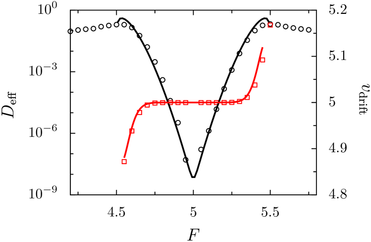
Figure 2: Simulation of Eq. 1 at the 1:1 synchronization ($\Omega=5.0$, $D=0.05$): $D_{\textrm{eff}}$ (circles) and the $v_{\textrm{drift}}$ (squares). The solid lines are the corresponding analytical results for the mean velocity (Stratonovich Stratonovich (1967)) and the effective diffusion from Eq. 7.

Please note that due to the assumptions the equation holds only in the limit of fast oscillations with respect to the intrinsic relaxation time $\Omega\gg\tau_{r}^{-1}$. Thus at 1:1 synchronization ($F=\Omega$, $\Omega\gg 1$) we are in fact in the super-critical force regime. In the co-moving frame even for $F>F_{\textrm{crit}}=1$ the reduced Equation 6 describes a particle moving in a tilted stationary periodic potential.

An analytical solution for $v_{\textrm{drift}}$ close to synchronization can be taken directly from the classical work of Stratonovich on the mean phase of an entrained stochastic oscillator Stratonovich (1967), whereas $D_{\textrm{eff}}$ can be calculated in the case of small noise $D\ll 1/2$, from the Kramers rates $k^{\pm}$ to neighboring minima of the co-moving stationary potential $D_{\textrm{eff}}=\frac{\lambda^{2}}{2}\left(k^{+}+k^{-}\right)$:

$$D_{\textrm{eff}}=\frac{w_{0}}{2\pi}\,\textrm{cosh}\left(\frac{\Delta}{D}\pi\right)e^{-\frac{2}{D}(\Delta\textrm{arcsin}(2\Delta)+w_{0})},$$ (7)

with $w_{0}=\frac{1}{2}\sqrt{1-4\Delta^{2}}$.

The breakdown of effective diffusion in the synchronization regime correspond to giant Péclet numbers, which indicate a quasi-deterministic Brownian transport. For low noise strength ($D<0.01$) and an optimal choice of $F$ the system shows no dispersion even for extremely large times ($t>10^{5}T$, $\sim 10^{4}$ particles).

At low $\Omega$ ($<1$) the first synchronization regimes are located at subcritical forces $F<1$. The dynamics can be described as a slip and stick motion dominated by the oscillating barriers. We assume a $\delta$-peaked probability distribution at the begin of the sliding motion (slip phase) at the position $y_{0}$ corresponding to the fixed point where the particle is located at the begin of the step. As soon as temporal barriers occur, the particle relaxes at $y_{l}=l\lambda/2$ with $l=(2n+1)$ and $n\in\mathbb{N}$ (stick phase). The envelope of the $\delta$-like distributions of the relaxed particles is assumed to be Gaussian with a mean $\mu_{e}$ and width $S$. The probability to find the particle at the unstable fixed points $y_{m}$ with $m=2n$ at the end of the step vanishes.

The total probability to find the particle close to fixed point $y_{l}$ at the end of the step reads

$$w_{l}=\frac{1}{2}\left[\textrm{erf}\left(\frac{y-\mu_{e}}{\sqrt{2S\Delta\tau}}\right)\right]_{(l-1)\lambda/2}^{(l+1)\lambda/2}.$$ (8)

Thus we can formally calculate the mean position and the variance after a single step

$$\langle y_{e}\rangle =\sum_{n=-\infty}^{\infty}y_{2n+1}w_{2n+1},$$ (9)

$$\langle(y-\langle y_{e}\rangle)^{2}\rangle =\sum_{n=-\infty}^{\infty}\left(y_{2n+1}-\langle y_{e}\rangle\right)^{2}w_{2n+1},$$ (10)

with $y_{2n+1}=(n+\frac{1}{2})\lambda$. As the distribution $P_{e}(y)$ has a finite width and most of the probability will be concentrated within few minima of the potential around the mean $\mu_{e}$. It is sufficient to consider only a finite number of points $n\in[n_{min},n_{max}]$ around $\mu_{e}$ and calculate the mean position and the variance by renormalizing the probabilities accordingly $\tilde{w}_{2n+1}=w_{2n+1}/\sum_{n=n_{min}}^{n_{max}}w_{2n+1}$. With results obtained in Eqs. 9 and 10 we can calculate the mean drift and the effective diffusion as

$$v_{\textrm{drift}}=2\langle y_{e}\rangle/T,\,~{}~{}~{}D_{\textrm{eff}}=\langle(y-\langle y_{e}\rangle)^{2}\rangle/T\,.$$ (11)

The mean of the particle probability distribution moves in the direction of the bias with an effective force $G=G(F,\Omega)$ within a time interval $\Delta\tau(F,\Omega)$ caused by the combined effect of the constant bias $F$ and the oscillating potential. The time of vanishing barriers is $\Delta\tau=2\arcsin(F)/\Omega$ and for $G$ we choose a linear dependence on $F$: $G(F)=aF$. Averaging over the potential oscillations leads to $a=1$.

The diffusion coefficient $S$ in Eq. 8 depends on the applied force and shows a large increase close to the critical force $F_{\textrm{crit}}$ likewise reported in Reimann et al. (2001). For simplicity we assume here a linear increase $S=bF$. The simplified theory given in Eqs. 8, 11 is compared with simulations of the full system for $\Omega=0.03,0.05$ in Fig. 3. Symbols represent the numerical results while the black solid line represents the analytical calculation for $a=0.8$ and $b=0.04$. The multiple peaks of the Péclet number with decreasing magnitude are reproduced together with the shift of the peaks towards larger $F$ for increasing $\Omega$ which leads to a decrease in the number of peaks for $F<F_{\textrm{crit}}$. However the most obvious difference is the position and the height of the first peak of the Péclet number.

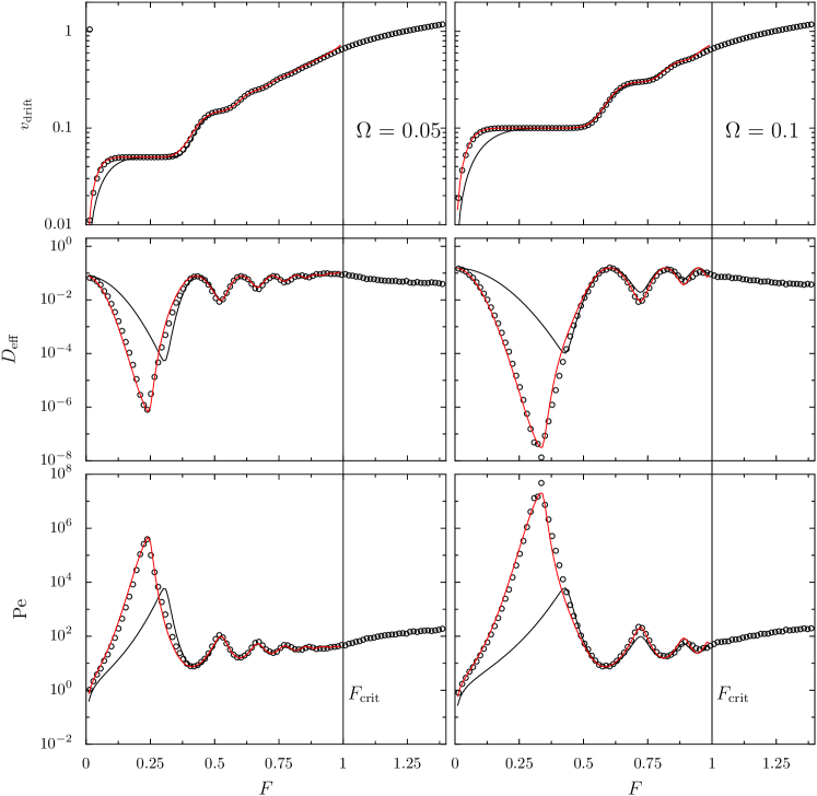
Figure 3: Comparison of simulations (symbols) with the theoretical results at low $\Omega$ (solid lines): mean velocity $v_{\textrm{drift}}$, effective diffusion $D_{\textrm{eff}}$ and Péclet number Pe vs. bias $F$ for $\Omega=0.05$ (left column) and $\Omega=0.1$ (right column). The black lines show the linear ansatz $G=aF$ with $a=0.8$, the red lines show the non-linear ansatz with $G=a(F)F$ with $a_{1}=1.6$, $a_{2}=0.8$, $c=10$ for both frequencies. The only changing parameter is $F_{t}$: for $\Omega=0.05$ $F_{t}=0.28$, for $\Omega=0.1$ $F_{t}=0.4$. For both examples shown $b=0.08$.

A small bias $F$ is potentiated by the slope of the oscillating potential therefore the parameter $a$ should be chosen as $a>1$. We describe this through a step function around $F_{t}$ as :$a(F)=a_{2}+(a_{1}-a_{2})\left[\textrm{tanh}\left(c(F_{t}-F)\right)-1\right]/2$ This phenomenological modification of the model leads to the red (gray) line and shows agreement to the numerical simulations. Please note that $F_{t}$ is the only changing parameter in calculations of the non-linear ansatz for different frequencies. This good agreement of the theoretical results with the numerical simulations shows that the theory accounts for the decisive mechanism responsible for the observed behavior: the combination of transport (slip phase) with repeated confinement (stick phase) at temporal minimum of the potential.

In this work we have analyzed the impact of a spatio-temporal oscillating potential on Brownian transport. We have demonstrated how the oscillating potential may enhance or suppress the effective diffusion. We derived an expression for $D_{\textrm{eff}}(\Omega,D)$ for vanishing bias $F=0$. We have obtained an optimal driving frequency which maximizes the diffusive transport. For finite bias $F>0$ we have shown the occurrence of synchronization regimes, with strongly suppressed effective diffusion and quasi-deterministic transport at finite noise strengths revealed through giant Péclet numbers.

Via a transformation to the co-moving frame at fast oscillations analytical expression based on previous results by Stratonovich and Kramers are found for the effective diffusion and mean velocity. At low frequencies we describe the system dynamics through a simplified ansatz of the transport process, which for reasonable choice of effective parameters are in agreement with the numerical results for $0<F<F_{\textrm{crit}}$. Our results suggest that in the unbiased case the introduction of an spatio-temporal periodic force enhance the diffusive transport, whereas for a finite bias it may significantly improve the quality of directed Brownian transport by suppressing thermal fluctuations.

The authors thank M. Kostur for the introduction to computing with CUDA NVIDIA (2009), which allowed a remarkable simulation speed up Januszewski and Kostur (2010). We acknowledge the financial support by the DFG through Sfb555.

References

- Reimann et al. (2001) P. Reimann et al., Phys. Rev. Lett. 87, 010602 (2001).
- Lindenberg (2007) K. Lindenberg et al., Phys. Rev. Lett. 98, 020602 (2007).
- (3) M. Borromeo and F. Marchesoni, Phys. Rev. E 78, 051125 (2008).
- Reimann (2002) P. Reimann, Physics Reports 361, 57 (2002).
- Anishchenko et al. (2002) V. S. Anishchenko, V. V. Astakhov, T. E. Vadivasova, A. B. Neiman, and L. Schimansky-Geier, Nonlinear Dynamics of Chaotic and Stochastic Systems, Springer Series in Synergetics (Springer, Berlin Heidelberg, 2002).
- Hänggi and Marchesoni (2008) P. Hänggi and F. Marchesoni, Rev. Mod. Phys. 81, 387 (2008).
- Lindner and Schimansky-Geier (2002) B. Lindner and L. Schimansky-Geier, Phys. Rev Lett. 89, 230602 (2002).
- Ajdari and Prost (1991) A. Ajdari and J. Prost, Proc. Natl. Acad. Sci. U.S.A. 88, 4468 (1991).
- Faucheux et al. (1995) L. P. Faucheux et al., Phys. Rev. Lett. 74, 1504 (1995).
- Tatarkova et al. (2003) S. A. Tatarkova, W. Sibbett, and K. Dholakia, Phys. Rev. Lett. 91, 038101 (2003).
- Bleil et al. (2007) S. Bleil, P. Reimann, and C. Bechinger, Phys. Rev. E , 75, 031117 (2007).
- Kautz (1996) R. L. Kautz, Rep. Prog. Phys. 59, 935 (1996).
- Sterck et al. (2009) A. Sterck, D. Koelle, and R. Kleiner, Phys. Rev. Lett. 103 (2009).
- Tierno et al. (2008) P. Tierno et al., J. Phys. Chem. B 112, 3833 (2008).
- Auge et al. (2009) A. Auge et al., Appl. Phys. Lett. 94, 183507 (2009).
- Ermentrout and Kopell (1986) G. B. Ermentrout and N. Kopell, SIAM J. Appl. Math. 46, 233 (1986).
- Neiman and Russell (2005) A. B. Neiman and D. F. Russell, Phys. Rev. E 71, 061915 (2005).
- Freund and Schimansky-Geier (1999) J. A. Freund and L. Schimansky-Geier, Phys. Rev. E 60, 1304 (1999).
- Stratonovich (1967) R. L. Stratonovich, Topics in the theory of random noise (Routledge, 1967).
- NVIDIA (2009) NVIDIA, NVIDIA CUDA Programming Guide 2.3.1 (2009), URL http://developer.nvidia.com/object/cuda_2_3_downloads.html.
- Januszewski and Kostur (2010) M. Januszewski and M. Kostur, Comput. Phys. Commun. 181, 183 (2010).