A Natural Symmetrization for the Plummer Potential

Abstract

We propose a symmetrized form of the softened gravitational potential which is a natural extension of the Plummer potential. The gravitational potential at the position of particle $i$ $(x_{i},y_{i},z_{i})$, induced by particle $j$ at $(x_{j},y_{j},z_{j})$, is given by:

$$\phi_{ij}=-\frac{Gm_{j}}{|{r_{ij}}^{2}+{\epsilon_{i}}^{2}+{\epsilon_{j}}^{2}|^{1/2}},$$

where $G$ is the gravitational constant, $m_{j}$ is the mass of particle $j$, $r_{ij}=|{(x_{i}-x_{j})^{2}+(y_{i}-y_{j})^{2}+(z_{i}-z_{j})^{2}}|^{1/2}$ and $\epsilon_{i}$ and $\epsilon_{j}$ are the gravitational softening lengths of particles $i$ and $j$, respectively. This form is formally an extension of the Newtonian potential to five dimensions. The derivative of this equation in the $x,y$, and $z$ directions correspond to the gravitational accelerations in these directions and these are always symmetric between two particles.

When one applies this potential to a group of particles with different softening lengths, as is the case with a tree code, an averaged gravitational softening length for the group can be used. We find that the most suitable averaged softening length for a group of particles is $\langle{\epsilon_{j}}^{2}\rangle=\sum_{j}^{N}m_{j}{\epsilon_{j}}^{2}/M$, where $M=\sum_{j}^{N}m_{j}$ and $N$ are the mass and number of all particles in the group, respectively. The leading error related to the softening length is $\mathcal{O}\left(\sum_{j}{{\boldsymbol{r}}_{j}d(\epsilon_{j}}^{2})/{{r_{ij}}^{3}}\right)$, where ${\boldsymbol{r}}_{j}$ is the distance between particle $j$ and the center of mass of the group and ${d(\epsilon_{j}}^{2})={\epsilon_{j}}^{2}-\langle{\epsilon_{j}}^{2}\rangle$. Using this averaged gravitational softening length with the tree method, one can use a single tree to evaluate the gravitational forces for a system of particles with a wide variety of gravitational softening lengths. Consequently, this will reduce the calculation cost of the gravitational force for such a system with different softenings without the need for complicated forms of softening. We present the result of simple numerical tests. We found that our modification of the Plummer potential works well.

1 Introduction

Aarseth (1963) introduced a Plummer potential (Plummer, 1911) for gravitational $N$-body simulations in order to eliminate the divergence of the potential that occurs when two particles undergo a close encounter. With a Plummer softening, the modified gravitational potential between two particles $i$ and $j$ is given by

$${\phi}_{ij}=-\frac{Gm_{j}}{|{{\boldsymbol{r}}_{ij}}^{2}+{\epsilon}^{2}|^{1/2}},$$ (1)

where $G$, ${\boldsymbol{r}}_{ij}$, $m_{j}$, and $\epsilon$ are the gravitational constant, the distance between particles $i$ and $j$, the mass of particle $j$ and the gravitational softening length, respectively. The increase in the calculation cost due to this modification of the potential is quite small. Thus, it is widely used in simulations of self-gravitating systems and the GRAPE (GRAvity PipE) series also adopts this form of the gravitational potential (Sugimoto et al., 1990; Ito et al., 1991; Okumura et al., 1993; Makino et al., 1997; Kawai et al., 2000; Makino et al., 2003; Kawai & Fukushige, 2006; Makino, 2005, 2007). Due to the wide adoption of the Plummer potential, there have been several studies on the choice of the optimal gravitational softening length (Merritt, 1996; Athanassoula et al., 2000; Dehnen, 2001).

In simulations of self-gravitating systems, it is necessary to deal with a wide range in both space and time. For example, one needs to cover the range of $\sim 100~{}{\rm Mpc}$ (for the tidal field) to $\sim 10~{}{\rm pc}$ or less (for the structure of the interstellar medium) in galaxy formation simulations . Usually, the outer region of the target galaxy is represented by massive particles in order to reduce the calculation cost (e.g., Navarro & Benz, 1991; Katz & White, 1993). In simulations of the coevolution of the galactic center and star cluster, it is necessary to use different masses for different components, since required accuracies and spatial resolutions are different (Fujii et al., 2007, 2010). Thus we need to use different gravitational softening lengths for different types of particles.

If one uses the direct summation method to calculate the gravitational force, it is possible to use an arbitrary symmetric form for the softening length; for example, $[({\epsilon_{i}}^{2}+{\epsilon_{j}}^{2})/2]^{1/2}$, $(\epsilon_{i}+\epsilon_{j})/2$, or $\max(\epsilon_{i},\epsilon_{j})$. On the other hand, when one uses the tree method (Appel, 1985; Barnes & Hut, 1986), one needs to use separate trees for each of the different groups of particles with the same gravitational softening length (e.g. Springel et al., 2001), since otherwise there will be an error in the force calculation of the order $\epsilon^{2}$. If one were to calculate the force from the center of mass of two particles with widely different gravitational softening values, it is not clear how one would take into account the gravitational softening length. However, if one uses different trees for particles with different gravitational softening lengths, the calculation cost increases by a large factor.

Hernquist & Katz (1989) proposed a different approach for softening. They assumed that each particle has a finite size and mass distribution given by a function with a compact support, e.g. a spline function. The advantage of this gravity kernel is that it becomes a purely Keplarian potential for distances larger than the particle size. Thus, for particles separated by distances larger than their sizes, one can use the center-of-mass approximation or the multipole expansion of a purely Keplarian potential. However, spline functions require a few conditional branches and the evaluation of a polynomial. These operations lead to a non-negligible slowdown in the force and potential calculations on modern CPUs/GPUs which have SIMD execution units. As a result, the calculation cost of a spline function is higher than that of the simple Plummer softening. Moreover, the tree approximation cannot be used for particles within the softening length. Thus, if there are many particles within the softening length, they can cause a large increase in the calculation cost.

In this paper, we propose a symmetrized gravitational potential between two particles with different softenings, which is a natural extension of the Plummer potential. We derive the multipole expansion of a group of such particles with this symmetrized potential. We then show that, in terms of accuracy, it is the best to use the second moment of the softening lengths of the particles in order to obtain the averaged softening length for the group. The multipole moment up to the second order has a simple form, which is easy and inexpensive to calculate.

This paper is structured as follows: in section 2, we present a symmetrized gravitational potential for a pair of particles with different gravitational softening lengths and then introduce an averaged gravitational softening length for a group of such particles. The use of this potential with the tree method is also discussed in the section. Results of numerical tests are given in section 3. A summary and discussion are shown in section 4.

2 Symmetrized Plummer Potential and its Applications to the Tree Code

2.1 Symmetrized Pairwise Potential

We modify the Plummer potential (Eq. 1) so that it is symmetric between two particles even when their gravitational softening lengths are different. Here, we consider the following form:

$${\phi}_{ij}=-\frac{Gm_{j}}{|{{\boldsymbol{r}}_{ij}}^{2}+{\epsilon_{i}}^{2}+{\epsilon_{j}}^{2}|^{1/2}}.$$ (2)

Formally, this form can be regarded as the $1/r$ potential in the five dimensional space ($x,y,z,\epsilon_{i},\epsilon_{j}$). This form has been used before to model the gravitational interaction between galaxy particles with different size and mass (White, 1976; Aarseth & Fall, 1980). When we take the gradients of Eq. 2 in the $x,y$ and $z$ directions, we obtain the gravitational accelerations, i.e.

$$a_{{ij},x} = -\frac{\partial\phi_{ij}}{\partial x},$$ (3)

$$= -\frac{Gm_{j}(x_{i}-x_{j})}{|{{\boldsymbol{r}}_{ij}}^{2}+{\epsilon_{i}}^{2}+{\epsilon_{j}}^{2}|^{3/2}}.$$

This gravitational acceleration satisfies Newton’s third law.

2.2 Multipole Expansion of the Potential of a Group of Particles with the Symmetrized Plummer Potential

In this section, we derive the multipole expansion of the gravitational potential for a group of particles with the symmetrized Plummer potential by introducing an averaged softening for the group of particles. Using Eq. 2, we obtain the most suitable form of the averaged softening which minimizes the potential/force error. This form can easily be used with a tree code (Barnes & Hut, 1986).

We consider the gravitational potential at ${\boldsymbol{r}}_{i}$ due to a group of particles $j=1,\dots,N$ with the total mass $M$. The three-dimensional position of particle $j$ is expressed as ${\boldsymbol{r}}_{j}$. Here we choose the center of mass of particles $j$ as the coordinate center. By taking the summation over $j$, the potential at ${\boldsymbol{r}}_{i}$ is

$${\phi}_{i}=-\sum_{j}^{N}\frac{Gm_{j}}{|{{\boldsymbol{r}}_{ij}}^{2}+{\epsilon_{i}}^{2}+{\epsilon_{j}}^{2}|^{1/2}},$$ (4)

where ${\boldsymbol{r}}_{ij}={\boldsymbol{r}}_{i}-{\boldsymbol{r}}_{j}$.

We consider the following form as the monopole potential of the group:

$${\phi^{\prime}}_{i}=-\frac{GM}{|{{\boldsymbol{r}}_{i}}^{2}+{\epsilon_{i}}^{2}+{\mathcal{E}_{j}}^{2}|^{1/2}},$$ (5)

where ${\mathcal{E}_{j}}^{2}$ is an arbitrary form of the averaged softening length for the group of particles $j$. As shown below, in terms of accuracy, we can obtain the most suitable form of the averaged softening length for the group of particles.

By using ${\mathcal{E}_{j}}^{2}$, we can rewrite Eq. 4 as follows:

$${\phi}_{i}=-\sum_{j}^{N}\frac{Gm_{j}}{|({{\boldsymbol{r}}_{i}-{\boldsymbol{r}}_{j}})^{2}+{\epsilon_{i}}^{2}+{\mathcal{E}_{j}}^{2}+d({\epsilon_{j}}^{2})|^{1/2}},$$ (6)

where $d({\epsilon_{j}}^{2})={\epsilon_{j}}^{2}-{\mathcal{E}_{j}}^{2}$. The Taylor expansion of Eq. 6 up to the second order of ${\boldsymbol{r}}_{j}$ and $d({\epsilon_{j}}^{2})$ is

$${\phi}_{i} = -\sum_{j}^{N}\frac{Gm_{j}}{R}\Biggl{\{}1+\frac{({\boldsymbol{r}}_{i}\cdot{\boldsymbol{r}}_{j})}{{R}^{2}}+\frac{d({\epsilon_{j}}^{2})}{{R}^{2}}$$ (7)

$$+\frac{3({\boldsymbol{r}}_{i}\cdot{\boldsymbol{r}}_{j})^{2}-|{\boldsymbol{r}}_{i}|^{2}|{\boldsymbol{r}}_{j}|^{2}}{{R}^{4}}+\frac{3({\boldsymbol{r}}_{i}\cdot{\boldsymbol{r}}_{j})d({\epsilon_{j}}^{2})}{{R}^{4}}$$

$$+\frac{3\left[d({\epsilon_{j}}^{2})\right]^{2}}{4{R}^{4}}+\mathcal{O}\left(\left[\frac{{\boldsymbol{r}}_{j}}{R}+\frac{d({\epsilon_{j}}^{2})}{R^{2}}\right]^{3}\right)\Biggl{\}}$$

where

$$R=\left({{\boldsymbol{r}}_{i}}^{2}+{\epsilon_{i}}^{2}+{\mathcal{E}_{j}}^{2}\right)^{1/2}.$$ (8)

The zeroth term of the Taylor expansion is ${\phi^{\prime}}_{i}$ itself (Eq. 5). The term of the order of $({\boldsymbol{r}}_{i}\cdot{\boldsymbol{r}}_{j})$ vanishes by definition. Since $d({\epsilon_{j}}^{2})={\epsilon_{j}}^{2}-{\mathcal{E}_{j}}^{2}$, the first order term of $d({\epsilon_{j}}^{2})$ vanishes if we adopt the second moment of $\epsilon_{j}$ as the averaged softening length:

$${\mathcal{E}_{j}}^{2}=\langle\epsilon_{j}^{2}\rangle\equiv\frac{\sum_{j}^{N}m_{j}{\epsilon_{j}}^{2}}{M}.$$ (9)

Hence, choosing the second moment of $\epsilon_{j}$ to be the averaged softening length is the most favourable option; using other forms such as $(\epsilon_{i}+\epsilon_{j})/2$, $\max(\epsilon_{i},\epsilon_{j})$ and $\min(\epsilon_{i},\epsilon_{j})$ result in a second-order error term.

For the convergence of the multipole expansion, it is necessary to take into account not only the ordinary three-dimensional distance but also the distribution of the softenings, $\epsilon_{j}$. We will discuss this point in the next subsection.

2.3 The opening criterion

In the tree method, the force and potential of a group of particles are approximated by that of the corresponding tree node. The opening criterion (Barnes & Hut, 1986),

$$\theta>\frac{w}{d},$$ (10)

is widely used to determine whether the multipole approximation can be used or not. Here, $\theta$ is called the opening angle and controls the force/potential accuracies, $w$ is the size of the tree node and $d$ is the distance between the barycenter of the tree node and the position where we want to calculate the force and potential. Since the multipole expansion of the $1/r$ potential around $r+dr$ is a series of $dr/r$ where $dr\sim w$ and $r\sim d$, Eq. 10 corresponds to the convergence condition for the multipole expansion of the $1/r$ potential. For the Plummer potential, the Plummer distance, $(r^{2}+{\epsilon_{i}}^{2})^{1/2}$, is adopted instead of $r$. Typically, a value of $\theta=0.5\sim 0.75$ is used. Note that, unless $\theta\leq 1/\sqrt{3}$, the Barnes & Hut’s opening criterion causes unbound errors in force calculation, resulting in “detonating galaxies” (Salmon & Warren, 1994). They studied other opening criteria so that one can avoid these large errors. Here, we use Eq. 10 with sufficiently small $\theta$. Hence our results, which will appear in section 3.3, are free from this problem.

As shown in section 2.2, the potential induced by a group of particles with the symmetrized form of the potential is expanded by two parameters, ${\boldsymbol{r}}_{j}$ and ${d\epsilon_{j}}^{2}$. Thus, the following two constraints together should satisfy the conditions for convergence:

$$\eta>\frac{|{\boldsymbol{r}}_{j}|}{R},$$ (11)

and

$$\eta^{\prime}>\frac{d({\epsilon_{j}}^{2})}{R^{2}}.$$ (12)

Here, $\eta$ and $\eta^{\prime}$ are the tolerance parameters for the multipole expansion of the symmetrized Plummer potential. By replacing ${\boldsymbol{r}}_{j}$ with $w$ and ${d\epsilon_{j}}^{2}$ with ${\epsilon_{\rm{max}}}^{2}-{\epsilon_{\rm{min}}}^{2}$, where $\epsilon_{\rm{max}}$ and $\epsilon_{\rm{min}}$ are the maximum and minimum softening lengths in a tree node, respectively, we obtain

$$\eta>\frac{w}{R},$$ (13)

and

$$\eta^{\prime}>\frac{{\epsilon_{\rm{max}}}^{2}-{\epsilon_{\rm{min}}}^{2}}{R^{2}},$$ (14)

for the convergence conditions of the multipole expansion.

Note that ${\epsilon_{\rm max}}^{2}-{\epsilon_{\rm min}}^{2}$ corresponds to the size of the “box” in the fifth dimension. In our current implementation, the tree structure is still an oct-tree in three dimensions. Thus, if a node contains two particles which have widely different gravitational softening lengths, its “size” can be dominated by the softening if its physical size is small. When we calculate the force from this node to a nearby particle with a distance $\leq[({\epsilon_{\rm max}}^{2}-{\epsilon_{\rm min}}^{2})/\eta^{\prime}]^{1/2}$, this node is always opened up even if the physical size of the node in three dimensions is much smaller than the distance. This behavior could cause an unnecessary increase in the calculation cost. In principle, we can easily solve this problem by making a tree structure in four-dimensional space, but so far we have not used such treatment.

In the tree-with-GRAPE method (Makino, 1991), a similar opening criterion, a set of Eqs 13 and 14, can be used with two modifications based on an argument for the convergence condition of the Taylor expansion. The modifications are as follows: First, we employ the minimum node-to-node distance in the ordinary three dimensions as the separation distance, ${\boldsymbol{r}}_{i}$, in Eq. 8. Then, we use the minimum gravitational softening length in the particles which share an interaction list, instead of $\epsilon_{i}$ in Eq. 8. These modifications give a sufficient accuracy when used with the tree-with-GRAPE method.

2.4 Calculation of averaged softening

The averaged gravitational softening length for each tree node can be calculated in the tree building phase with a recursive operation that is the same as that for the multipole expansion. The averaged gravitational softening length for a parent node, $\langle\epsilon_{p}^{2}\rangle$, is

$$\langle{{\epsilon}_{\rm p}}^{2}\rangle=\frac{\sum_{k}^{N_{\rm c}}M_{{\rm c},k}{{\langle{{\epsilon}_{{\rm c},k}}^{2}\rangle}}}{M_{\rm p}},$$ (15)

where $N_{\rm c}$ is the number of child nodes, $M_{\rm c,k}$ and $\langle{{\epsilon}_{{\rm c},k}}^{2}\rangle$ are the mass and the averaged gravitational softening length of the $k$-th child node, respectively, and $M_{\rm p}$ is the mass of the parent node.

2.5 Higher order expansion and application to FMM

In this section, we discuss the application of the symmetric softening to the fast multipole method (FMM) (Greengard & Rokhlin, 1987; Zhao, 1987; Dehnen, 2000). Unlike the tree method, in FMM, multipole expansions are first translated to local expansion, which is then evaluated at the positions of multiple particles. Thus, the calculation order in FMM is proportional to $N$.

The calculation cost in FMM depends on the expansion order of the multipole moments in the local/external particles. In the standard FMM (Greengard & Rokhlin, 1987), spherical harmonics is used to express expansion and thus the calculation cost is $\mathcal{O}(p^{4}N)$, where $p$ is the order of the multipole expansion. Elliott & Board (1996) successfully reduced the calculation cost in FMM from $\mathcal{O}(p^{4}N)$ to $\mathcal{O}(p(\log p)^{1/2}N)$ by using a fast fourier transformation and optimal choice of the tree level. Dehnen (2000) proposed a Cartesian FMM, however, its calculation cost is estimated as $O(p^{6}N)$. Again this cost can be reduced to $\mathcal{O}(p^{3/2}(\log p)^{1/2}N)$ by following Elliott & Board (1996).

With the $1/r$ potential in the five dimensions presented here, one cannot use a spherical harmonic function for the expansion. Thus, it is necessary to use a straightforward expansion such as what is used in the Cartesian FMM (Dehnen, 2000) to implement our symmetrized Plummer potential. In the multipole expansions, because it is necessary to expand the fourth or fifth dimension for the local and external field, the calculation cost is $\mathcal{O}(p^{8}N)$ and the reduced calculation cost is $\mathcal{O}(p^{2}(\log p)^{1/2}~{}N)$. When the multipole expansion is applied, the softening lengths of the particles are usually smaller than the size of the node and therefore one usually needs to take into account only the first cross term in Eq. 7. In this case, the calculation cost is similar to that of the Cartesian FMM. Moreover, gravitational softening is used in simulations where the required force accuracy is not very high. Therefore the multipole expansion can be truncated in relatively low orders. Thus, the increase in the calculation cost is not so large if one incorporates the symmetrized Plummer potential into FMM.

3 Tests

3.1 Error in Acceleration

Here, we present the measured acceleration error of the force calculated using a tree and our symmetrized form of the Plummer potential. We take two groups of $5\times 10^{4}$ particles, each with a different mass and softening length. The particles are randomly distributed within a uniform sphere of radius $L=1$. Table 1 shows the different combinations of masses and gravitational softening lengths used for this test. The accuracy of the accelerations depends strongly on the distribution of particles (Barnes & Hut, 1989). However, for simplicity, we consider only a uniform sphere here. In this test, we adopt the center-of-mass approximation for the force calculation and we use the set of Eqs 13 and 14 for the opening criterion. For this criterion, the tolerance is always kept the same and is represented by $\theta$ instead of $\eta$ and $\eta^{\prime}$ for simplicity.

Table 1: The summary of the masses and gravitational softening lengths of the two types of particles used in our test simulations. $m_{1}$ and $\epsilon_{1}$ refer to the mass and gravitational softening length for the less massive particles, whereas $m_{2}$ and $\epsilon_{2}$ are those of the massive particles. The number of particles in each group is $5\times 10^{4}$.

Mass ratio	$m_{1}$	$\epsilon_{1}$	$m_{2}$	$\epsilon_{2}$
$1:1$	$1.00\times 10^{-5}$	$6.79\times 10^{-3}$	$1.00\times 10^{-5}$	$6.79\times 10^{-3}$
$1:8$	$2.22\times 10^{-6}$	$4.11\times 10^{-3}$	$1.78\times 10^{-5}$	$8.22\times 10^{-3}$
$1:64$	$3.08\times 10^{-7}$	$2.13\times 10^{-3}$	$1.97\times 10^{-5}$	$8.51\times 10^{-3}$

We measure the mean acceleration error as a function of the opening angle for the three different mass ratios: 1:1, 1:8 and 1:64 (see Table 1). The mean acceleration error for each case is given by the following equation:

$$\langle\Delta a(\theta)\rangle=\frac{1}{N}\sum^{N}_{i}\frac{\left|{\boldsymbol{a}}_{i}(\theta)-{\boldsymbol{a}}_{i,0}\right|}{\left|{\boldsymbol{a}}_{i,0}\right|},$$ (16)

where ${\boldsymbol{a}}_{i}(\theta)$ is the acceleration vector of particle $i$ estimated with tolerance $\theta$ and ${\boldsymbol{a}}_{i,0}$ is that evaluated for $\theta=0$. We also measure the mean acceleration error which excludes the error due to $d(\epsilon^{2})$. To do this, we build two trees, where each tree consists of particles with the same mass and softening. We then calculate the accelerations of the particles by adding the forces from the two trees so that we obtain the mean acceleration error without the contribution of $d(\epsilon^{2})$.

The mean acceleration error as a function of $\theta$, for each of these methods, is shown in Figure 1. We found that there is no clear difference in the mean acceleration errors between different methods. We also found that the mean acceleration error is approximately proportional to $\theta^{3}$. This is in good agreement with previous results obtained by the tree code with the usual Plummer potential (Hernquist, 1987; Barnes & Hut, 1989; Makino, 1990). This means that our adopted opening criteria work correctly.

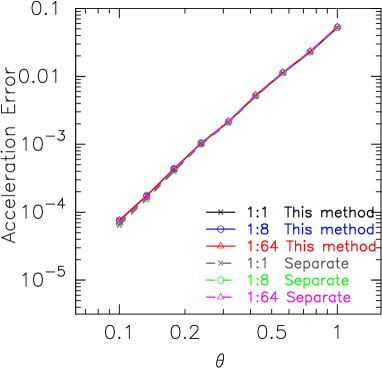
Figure 1: Mean acceleration error as a function of the tolerance parameter $\theta$. Curves with crosses, circles and triangles are the results for $m_{2}/m_{1}=1,8$ and $64$, respectively. The solid and dashed curves are the results obtained by the tree which uses our averaged softening length (“This method”), whilst the dashed curves are those obtained from using two separate trees, where each tree consists of each particle group (“Separate”).

3.2 Calculation Cost

To evaluate the calculation cost, we measured the average number of particle-particle interactions and the average number of total interactions. Figure 2 shows the these numbers as a function of $\theta$. We used the same distribution of particles as we used in section 3.1. The dotted curves are the calculation cost for the case of two separate trees for particles with different softenings. The calculation cost of our method is about one half of that of the calculation with two separate trees. The average number of the interactions is roughly proportional to $\theta^{-3}$ for both methods. This dependence is again close to those in previous works (Makino, 1990).

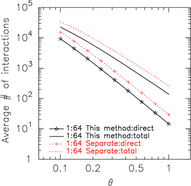
Figure 2: Number of the average interactions as a function of $\theta$ with $L=1$ and $m_{2}/m_{1}=64$. Curves with symbols are the number of the mean particle-particle interactions, whereas curves without symbols are the sum of the number of the mean particle-particle and mean particle-node interactions.

3.3 Energy Error in Time Integration

Here, we present the result of test calculations of a cold collapse. We create a uniform sphere with the radius $L$ and mass $M$ using a random distribution of $1024$ particles, where the system of units we use is $L=M=G=1$. The sphere consists of two groups of $512$ particles. The mass and softening length of particles in these two groups are varied and the values used are given in Table 2. The initial virial ratio of the system was set to $0.1$ and the initial particle velocities were drawn from a Gaussian distribution.

Table 2: The same as table 1 but for the test calculations of cold collapse.

Mass ratio	$m_{1}$	$\epsilon_{1}$	$m_{2}$	$\epsilon_{2}$
$1:1$	$9.77\times 10^{-4}$	$3.13\times 10^{-2}$	$9.77\times 10^{-4}$	$3.13\times 10^{-2}$
$1:8$	$2.17\times 10^{-4}$	$1.89\times 10^{-2}$	$1.74\times 10^{-3}$	$3.79\times 10^{-2}$
$1:64$	$3.00\times 10^{-5}$	$9.79\times 10^{-3}$	$1.92\times 10^{-3}$	$3.92\times 10^{-2}$

The numerical simulations were performed using ASURA (Saitoh, in preparation). ASURA adopts the tree-with-GRAPE method to calculate the gravitational force and potential (Makino, 1991). For this test, ASURA only uses the center-of-mass of the tree nodes to calculate the force, with their averaged gravitational softening lengths determined according to Eq. 9 and the tolerance is set to $0.5$. The maximum number of particles which shares the same interaction list (Barnes, 1990; Makino, 1991) was set to $n_{\rm g}=8$ and $n_{\rm g}=128$. Time-integration scheme used is an ordinary leap-frog method.

Figure 3 shows the relative error in the total energy of the system, $\Delta E$, at time $t=1$ (which is approximately the time of maximum collapse) as a function of the size of the time-step. Here $\Delta E$ is defined as

$$\Delta E=\left|\frac{E(t=0)-E(t=1)}{E(t=0)}\right|,$$ (17)

where $E(t)$ is the total energy of the system at $t$.

From figure 3, we can see that the mass ratio between groups of particles does not affect the relative error. For small time-steps ($\leq 2^{-6}$), the relative error of the tree method is larger than that of the direct method. This is because the error in the calculated force from using a tree dominates the integration error. The contribution of the tree approximation to the relative error is smaller for large $n_{\rm g}$, since a larger number of nearby particles is included in the direct calculation (Barnes, 1990).

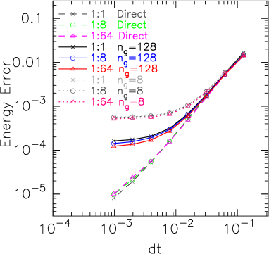
Figure 3: Dependence of the relative energy error (at time $t=1$) on time-step size. Crosses, circles and triangles are the results for $m_{2}/m_{1}=1,8$ and $64$, respectively. Solid, dotted, and dashed curves are the results for $n_{\rm g}=128$, $n_{\rm g}=8$, and direct calculation, respectively.

4 Summary and Discussion

In this paper, we introduced a natural symmetrization of the Plummer potential. This symmetrization is quite simple and hence, easy for anyone to implement into their own code, providing their code adopts the traditional Plummer potential for gravity.

By applying this potential to a group of particles, we derived an averaged gravitational softening length for the group. Consequently, we can use this potential in the tree method. The multipole expansion of the symmetrized Plummer potential allows us to use a single tree to calculate forces and potentials for a system of particles that have different softening lengths. Thus the calculation cost of our method is less than that of previous implementations.

Since the modification is quite simple, the modified Plummer potential can be easily implemented in modern GRAPEs (i.e., GRAPE-7 and GRAPE-DR ) as they can modify the force law via software libraries. However, for older GRAPEs, the gravity pipelines are implemented on the hardware layer and so it is impossible to use this modified potential. The latest version of the GRAPE-DR library supports this new symmetrized Plummer potential.

Pure software libraries, i.e. those that run on typical CPUs without special hardware, can easily include our calculation model. Phantom-GRAPE (Nitadori et al, in preparation) is an optimized library that utilizes the SIMD instructions of X86 CPUs and has application interfaces comparable with GRAPE-5 (Kawai et al., 2000). For this software, we can easily modify the gravity kernel in the library. We used this modified Phantom-GRAPE for the tests described in Section 3.

The implementation of our modified Plummer potential on GPGPUs (Nakasato, 2009; Hamada et al., 2009) is also straightforward.

References

- Aarseth (1963) Aarseth, S. J. 1963, MNRAS, 126, 223
- Aarseth & Fall (1980) Aarseth, S. J., & Fall, S. M. 1980, ApJ, 236, 43
- Appel (1985) Appel, A. W. 1985, SIAM Journal on Scientific and Statistical Computing, 6, 85
- Athanassoula et al. (2000) Athanassoula, E., Fady, E., Lambert, J. C., & Bosma, A. 2000, MNRAS, 314, 475
- Barnes & Hut (1986) Barnes, J., & Hut, P. 1986, Nature, 324, 446
- Barnes (1990) Barnes, J. E. 1990, J. Comput. Phys., 87, 161
- Barnes & Hut (1989) Barnes, J. E., & Hut, P. 1989, ApJS, 70, 389
- Dehnen (2000) Dehnen, W. 2000, ApJL, 536, L39
- Dehnen (2001) —. 2001, MNRAS, 324, 273
- Elliott & Board (1996) Elliott, W. D., & Board, Jr., J. A. 1996, SIAM J. Sci. Comput., 17, 398
- Fujii et al. (2007) Fujii, M., Iwasawa, M., Funato, Y., & Makino, J. 2007, PASJ, 59, 1095
- Fujii et al. (2010) —. 2010, ApJL, 716, L80
- Greengard & Rokhlin (1987) Greengard, L., & Rokhlin, V. 1987, Journal of Computational Physics, 73, 325
- Hamada et al. (2009) Hamada, T., Narumi, T., Yokota, R., Yasuoka, K., Nitadori, K., & Taiji, M. 2009, in SC ’09: Proceedings of the Conference on High Performance Computing Networking, Storage and Analysis (New York, NY, USA: ACM), 1–12
- Hernquist (1987) Hernquist, L. 1987, ApJS, 64, 715
- Hernquist & Katz (1989) Hernquist, L., & Katz, N. 1989, ApJS, 70, 419
- Ito et al. (1991) Ito, T., Ebisuzaki, T., Makino, J., & Sugimoto, D. 1991, PASJ, 43, 547
- Katz & White (1993) Katz, N., & White, S. D. M. 1993, ApJ, 412, 455
- Kawai & Fukushige (2006) Kawai, A., & Fukushige, T. 2006, in SC ’06: Proceedings of the 2006 ACM/IEEE conference on Supercomputing (New York, NY, USA: ACM), 48
- Kawai et al. (2000) Kawai, A., Fukushige, T., Makino, J., & Taiji, M. 2000, PASJ, 52, 659
- Makino (1990) Makino, J. 1990, J. Comput. Phys., 88, 393
- Makino (1991) Makino, J. 1991, PASJ, 43, 621
- Makino (2005) —. 2005, ArXiv Astrophysics e-prints:0509278
- Makino (2007) —. 2007, Highlights of Astronomy, 14, 424
- Makino et al. (2003) Makino, J., Fukushige, T., Koga, M., & Namura, K. 2003, PASJ, 55, 1163
- Makino et al. (2007) Makino, J., Hiraki, K., & Inaba, M. 2007, in SC ’07: Proceedings of the 2007 ACM/IEEE conference on Supercomputing (New York, NY, USA: ACM), 1–11
- Makino et al. (1997) Makino, J., Taiji, M., Ebisuzaki, T., & Sugimoto, D. 1997, ApJ, 480, 432
- Merritt (1996) Merritt, D. 1996, AJ, 111, 2462
- Nakasato (2009) Nakasato, N. 2009, ArXiv Astrophysics e-prints:0909.0541
- Navarro & Benz (1991) Navarro, J. F., & Benz, W. 1991, ApJ, 380, 320
- Okumura et al. (1993) Okumura, S. K. et al. 1993, PASJ, 45, 329
- Plummer (1911) Plummer, H. C. 1911, MNRAS, 71, 460
- Salmon & Warren (1994) Salmon, J. K., & Warren, M. S. 1994, J. Comp. Phys, 111, 136
- Springel et al. (2001) Springel, V., Yoshida, N., & White, S. D. M. 2001, New Astronomy, 6, 79
- Sugimoto et al. (1990) Sugimoto, D., Chikada, Y., Makino, J., Ito, T., Ebisuzaki, T., & Umemura, M. 1990, Nature, 345, 33
- White (1976) White, S. D. M. 1976, MNRAS, 177, 717
- Zhao (1987) Zhao, F. 1987, An Algorithm for Three-Dimensional -body Simulations, Tech. rep., Cambridge, MA, USA