Interplay between spin density wave and $\pi$ phase shifted superconductivity in the Fe pnictide superconductors

Abstract

We explore if the phase separation or coexistence of the spin density wave (SDW) and superconductivity (SC) states has any relation to the incommensurability of the SDW in the Fe pnictide superconductors. A systematic method of determining the phase separation or coexistence was employed by computing the anisotropy coefficient $\beta$ from the the 4th order terms of the Ginzburg–Landau (GL) expansion of the free energy close to the tricritical/tetracritical point. It was complemented by the self-consistent numerical iterations of the gap equations to map out the boundaries between the phase separation and coexistence of the SDW and SC phases, and between commensurate (C) and incommensurate (IC) SDW in the temperature–doping plane. Our principal results for the sign reversed $s$-wave pairing SC, in terms of the multicritical temperature, $T_{c}$, the phase separation/coexistence boundary between the SDW and SC, $T^{*}$, and the boundary between C/IC SDW, $T_{M}^{*}$, are: (a) IC-SDW and SC coexist for $T_{c}<T^{*}$ and phase separate otherwise, (b) SDW takes the C form for $T_{c}>T_{M}^{*}$ and IC form for $T_{c}<T_{M}^{*}$, and (c) the thermodynamic first order phase transition intervenes in between the C-SDW and IC-SDW boundary for large $T_{M}^{0}$, where $T_{M}^{0}$ is the SDW transition temperature at zero doping, $T^{*}=0.35~{}T_{M}^{0}$ and $T_{M}^{*}=0.56\ T_{M}^{0}$. The intervention makes the phase diagram more complicated than previously reported. By contrast no coexistence was found for the equal sign pairing SC. These results will be compared with the experimental reports in the Fe pnictide superconductors.

I Introduction

The alluring prospect of opening a key window to understanding the mechanism of high temperature superconductivity has attracted enormous research activities in the iron based pnictides.Kamihara et al. (2008); Chen et al. (2008a, b) A widespread school of thought regarding the pairing interaction maintains that magnetic fluctuations are intimately involved for the superconductivity. This view seems natural from the overall phase diagram of the pnictides in the temperature and doping plane. The superconductivity (SC) emerges out of the parent antiferromagnetic (AF) state as the static AF order is suppressed and charge carriers are introduced through the electron or hole doping in common with the cuprate high temperature superconductors.Fang et al. (2009) This view is further supported by the neutron scattering investigations showing a resonance at the wave vector related to the AF order coincident with the onset of superconductivity.Christianson et al. (2008)

The intimacy of SC and AF or spin density wave (SDW) states is a common feature among the unconventional superconductors like the cuprates, pnictides, and heavy fermion superconductors.Uemura (2009) It will, therefore, be important to understand the interplay between the SC and SDW orders. For the cuprates, it is perhaps one of the best established observations that the SC emerges out of AF parent state as the doping is introduced.Sanna et al. (2004) For the heavy fermion Ce115 compounds, the interplay between them has been studied actively for CeRhIn₅ and CeCoIn₅. For CeRhIn₅, for instance, the AF and SC phases coexist under pressure at zero magnetic field.Knebel et al. (2009); Park et al. (2006) Within the coexisting dome, the AF changes from incommensurate (IC) to commensurate (C) SDW as the pressure is increased.Yashima et al. (2009)

Experimental investigations on the interplay between the SC and SDW for the pnictides report diverse results with regard to the pnictide families and the dopants. For the 1111 family, Luetkens $et~{}al.$Luetkens et al. (2009) reported from the muon spin relaxation ($\mu$SR) and Mössbauer spectroscopy on the LaFeAsF_xO_1-x (La1111) compounds that the magnetic state disappears and superconductivity emerges abruptly as the doping $x$ is increased. For Sm1111 system, Drew $et~{}al.$ found that the AF and SC regions coexist which could be due to phase separation.Drew et al. (2009) The neutron scattering measurements for the Ce1111 compounds reported a magnetic phase diagram similar to La1111.Zhao et al. (2008) For the 122 family, Laplace $et~{}al.$Laplace et al. (2009) reported that the IC-SDW coexists with the SC on the atomic scale in Ba(Fe_1-xCo_x)₂As₂ compounds by measuring ⁷⁵As nuclear magnetic resonance (NMR) and susceptibility. Julien $et~{}al.$Julien et al. (2009) contrasted K and Co doped 122 compounds by also measuring ⁷⁵As NMR and found that the SC and SDW phase separate for Ba_0.6K_0.4Fe₂As₂ but microscopically coexist for Ba(Fe_1-xCo_x)₂As₂ in accord with Laplace $et~{}al.$ Parker $et~{}al.$Parker et al. (2010) reported from the neutron and muon experiments on NaFe_1-xM_xAs (M=Co, Ni) that the SC and SDW coexist on atomic level.

Theoretically the interplay between SC and SDW for the Fe pnictide superconductors was studied in a simple two band model by many groups.Vorontsov et al. (2009, 2010); Cvetkovic and Tesanovic (2009); Parker et al. (2009); Fernandes et al. (2010) They reported that the coexistence of SC and SDW is possible when SDW is IC for the $\pi$ phase shifted pairing. In this paper we also take the two band model to study the interplay between the SC and SDW. We make the Ginzburg-Landau (GL) expansion of the free energy close to the multicritical point for IC as well as C-SDW states. The nature of transitions was then determined from the 4th order terms, that is, whether they are continuous or discontinuous and whether the two orders coexist or phase separate. The phase separation or coexistence was determined by computing the anisotropy coefficient $\beta$ from the 4th order terms of the GL expansion for general IC SDW states. The superconducting state was modeled in terms of the sign reversed two band SC theory.Mazin et al. (2008); Kuroki et al. (2008); Bang and Choi (2008) The $0<\beta<1$ or not means phase coexistence or separation. See Eqs. (35) and (36) below. The multicritical temperature $T_{c}$ which equals to the superconducting critical temperature in the simple model we took is set by the interaction $\lambda_{S}$. The SDW transition temperature at zero doping $T_{M}^{0}\equiv T_{M}(\delta=0)$ is set by $\lambda_{M}$. $\delta$ is the deviation from the perfect nesting and may be tuned by doping or pressure.

When $\lambda_{M}$ is only slightly larger than $\lambda_{S}$, then $T_{M}^{0}/T_{c}\gtrsim 1$, and the multicritical point occurs at a small doping. The deviation from the perfect nesting is then small and the SDW takes the commensurate form. The computation of $\beta$ yields $\beta\geq 1$ which means that the C-SDW and SC phase separate. As the ratio of $T_{M}^{0}/T_{c}$ increases, $T_{M}(\delta)$ equals to $T_{c}$ at a larger $\delta$, and the SDW becomes IC for $T_{c}<T_{M}^{*}$. We use the notations that $T_{M}^{*}$ represents the boundary between C-SDW and IC-SDW determined by Eq. (22) and $T^{*}$ represents the phase separation/coexistence boundary between SDW and SC determined by Eq. (36) below. $T_{M}^{*}>T^{*}$ in our model. The IC-SDW and SC phases remain separated for $T_{c}>T^{*}$. For $T_{c}<T^{*}$, the $\beta$ becomes $0<\beta<1$ and the IC-SDW and SC phases coexist. We obtain $T_{M}^{*}=0.56\ T_{M}^{0}$ in agreement with Ref. Vorontsov et al. (2009), and $T^{*}=0.35\ T_{M}^{0}$. See Eqs. (40) and (42) below.

The SDW transition as $T$ is reduced is continuous for almost all of the parameter space. But, as the doping at the multicritical point is increased, the 4th order term of the SDW order $\beta_{M}$ of Eqs. (23) and (48) becomes negative and the first order transition intervenes in between the C-SDW and IC-SDW boundary. The intervention of the discontinuous transition makes the phase boundary more complicated. See the Fig. 1 and discussions below for details. Note that this 1st order transition is as the temperature is lowered as presented in Fig. 3. On the other hand, the 1st order transition between SDW and SC as $\delta$ is varied below $T_{c}$ corresponds to the phase separation as shown in Fig. 2.

The GL expansion was combined with the self-consistent numerical iterations of the gap equations to map out the boundary between the phase separation and coexistence of SDW and SC in the plane of $T$ and $\delta$ for the pnictide superconductors. See the the figures 2–4.

This paper is organized as follows: In the following section we will present the functional integral formulation of the Ginzburg–Landau free energy and the self-consistent gap equations from a simple two band model.Lee and Choi (2009) Then we introduce the anisotropy coefficient $\beta$ from the 4th order terms of the GL free energy which determines the phase separation or coexistence between the SDW and SC. In section III, we present the detailed calculations of the multicritical point, the coefficient $\beta$, and SDW and SC order parameters. We first show the multicritical point in the $T-\delta$ plane in Fig. 1 from which one can read off the nature of phase transitions. Then we present three typical cases: phase separated C-SDW and SC in Fig. 2, discontinuous SDW and SC phases in Fig. 3, and coexisting IC-SDW and SC phases in Fig. 4. These results will be commented in comparison with the experimental situations. Section IV is for summary and concluding remarks.

II Formalism

We take the following hamiltonian as with Ref. Vorontsov et al. (2009) to describe the interplay between superconductivity and antiferromagnetism.

$$H=\sum_{i,k,\sigma}\xi_{ik}c_{ik\sigma}^{\dagger}c_{ik\sigma}+H_{S}+H_{M},$$ (1)

$$H_{S}=\sum_{k,k^{\prime}}V_{S}\left[\ c_{1,k,\uparrow}^{\dagger}c_{1,-k,\downarrow}^{\dagger}c_{2,-k^{\prime},\downarrow}c_{2,k^{\prime},\uparrow}+h.c.\right],$$ (2)

$$H_{M}=-V_{M}\sum_{k,\sigma}\sigma c_{1,k,\sigma}^{\dagger}c_{2,k+q,\sigma}\sum_{k^{\prime},\sigma^{\prime}}\sigma^{\prime}c_{2,k^{\prime}+q,\sigma^{\prime}}^{\dagger}c_{1,k^{\prime},\sigma^{\prime}},$$ (3)

where the $V_{M}$ and $V_{S}$ are the magnetic and superconducting interaction strengths, respectively, and $q$ is the incommensurability of SDW. $q=0$ and $\neq 0$ represent the C and IC-SDW which is determined by maximizing the magnetic susceptibility $\chi(q)$. See Eq. (20) below.

The partition function of the Hamiltonian of Eq. (1) in the form of functional integral is given byNegele and Orland (1988) ($\tau$ is an imaginary time, and $\beta=1/k_{B}T$)

$$Z=$$

$$\int D[c_{1}^{\dagger},c_{2}^{\dagger},c_{1},c_{2}]\,e^{-\int_{0}^{\beta}\,d\tau\left[\sum_{k}(c_{1}^{\dagger}\partial_{\tau}c_{1}+c_{2}^{\dagger}\partial_{\tau}c_{2})+H(\tau)\right]}.$$

The next step is to employ the Hubbard-Stratonovich transformations to decouple the electron-electron interactions of $H_{S}$ and $H_{M}$. It is straightforward to obtainLee and Choi (2009)

$$e^{-\int_{0}^{\beta}d\tau H_{S}(\tau)}=\int D[\Delta_{1}^{*},\Delta_{2}^{*},\Delta_{1},\Delta_{2}]e^{-S_{S}},$$

$$e^{-\int_{0}^{\beta}d\tau H_{M}(\tau)}=\int D[m^{*},m]e^{-S_{M}},$$ (5)

where

$$S_{S} = \int d\tau\sum_{k}\,\left[-\frac{\Delta_{1}^{*}(\tau)\Delta_{2}(\tau)}{V_{S}}-\left\{c^{\dagger}_{1,k,\uparrow}(\tau)c^{\dagger}_{1,-k,\downarrow}(\tau)\Delta_{2}(\tau)\right.\right.$$ (6)

$$+ \left.\left.c^{\dagger}_{2,k,\uparrow}(\tau)c^{\dagger}_{2,-k\downarrow}(\tau)\Delta_{1}(\tau)+h.c.\right\}\right],$$

$$S_{M} = \int d\tau\sum_{k}\,\left[\frac{m^{*}(\tau)m(\tau)}{V_{M}}\right.$$ (7)

$$- \left.\left\{m(\tau)\sum_{\sigma}\sigma c_{1,k,\sigma}^{\dagger}(\tau)c_{2,k+q,\sigma}(\tau)+h.c.\right\}\right].$$

$\Delta_{1/2}(\tau)$ are nothing but the (fluctuating) superconducting order parameters. $\Delta_{1}$ and $\Delta_{2}$ are taken as the opposite sign in accord with the $s_{\pm}$ pairing.Mazin et al. (2008); Kuroki et al. (2008) It is more convenient to introduce

$$\Delta=\sqrt{-\Delta_{1}\Delta_{2}}$$ (8)

as with Ref. Lee and Choi (2009). Integrate out the fermions to get

$$Z[\Delta,m]=\int D[\Delta,m]\,e^{-F},$$

$$F = \int_{0}^{\beta}d\tau\Big{[}\int d\xi\,\frac{1}{V_{S}}\Delta^{*}(\tau)\Delta(\tau)$$

$$+\frac{1}{V_{M}}m^{*}(\tau)m(\tau)-\ln\det(\widehat{M}_{S}+\widehat{M}_{M})\Big{]}.$$

We then make the saddle point approximation which is determined by the condition that the first order functional derivative of the action $F$ with respect to $\Delta$ and $m$ vanish.

$$\left.\frac{\delta F}{\delta\Delta}\right|_{\Delta_{0},m_{0}}=\left.\frac{\delta F}{\delta m}\right|_{\Delta_{0},m_{0}}=0,$$ (10)

where $\Delta_{0},m_{0}$ denote the saddle point values. These functional derivatives can be computed using the following matrix identity

$$\delta\ln\det M=\delta\mathrm{Tr}\ln M=\mathrm{Tr}(M^{-1}\delta M).$$ (11)

They are, of course, the usual gap equations:Lee and Choi (2009)

$$\Delta=\sum_{\sigma=\pm}\frac{1}{2}\int_{-\omega_{c}}^{\omega_{c}}d\xi\lambda_{S}\frac{\Delta}{2E_{\sigma}}\tanh\left(\frac{E_{\sigma}}{2T}\right),$$ (12)

$$m=$$

$$\sum_{\sigma=\pm}\frac{1}{2}\int_{-\omega_{c}}^{\omega_{c}}d\xi\lambda_{M}\frac{m}{2E_{\sigma}}\left(1+\frac{\sigma\delta}{\sqrt{\xi^{2}+m^{2}}}\right)\tanh\left(\frac{E_{\sigma}}{2T}\right),$$

where the subscript $0$ was dropped,

$$\lambda_{S}=N_{F}V_{S},~{}~{}\lambda_{M}=N_{F}V_{M},$$ (14)

where $N_{F}$ is the density of states at the Fermi level, and the energies are given by

$$E_{\pm}=\sqrt{\left(\sqrt{m^{2}+\xi^{2}}\pm\delta\right)^{2}+\Delta^{2}}.$$ (15)

We took $\xi_{1k}=-\xi+\delta$ and $\xi_{2k}=\xi+\delta$ for the hole and electron Fermi surfaces, respectively.Vorontsov et al. (2009) The free energy is given as follows:

$$F=$$

$$\frac{1}{\lambda_{S}}\Delta^{*}\Delta+\frac{1}{\lambda_{M}}m^{*}m-2T\sum_{\nu=\pm}\sum_{k}\ln\cosh\left(\frac{1}{2}\beta E_{\nu,k}\right).$$

We take $\omega_{c}$ as the unit of energy ($\omega_{c}=1$).

The second order terms are

$$F^{(2)}=\left(\lambda_{M}^{-1}-\chi_{M}\right)m^{*}m+\left(\lambda_{S}^{-1}-\chi_{S}\right)\Delta^{*}\Delta,$$ (17)

where the pairing and magnetic susceptibilities are given by

$$\chi_{S}(T)=\frac{1}{2}\int_{-\omega_{c}}^{\omega_{c}}d\xi\frac{1}{\xi}\tanh\left(\frac{\xi}{2T}\right),$$ (18)

$$\chi_{M}(\delta,T)=\frac{1}{2}\int_{-\omega_{c}}^{\omega_{c}}d\xi\frac{1}{\xi}\tanh\left(\frac{\xi+\delta}{2T}\right).$$ (19)

When the doping is increased the magnetic transition may be incommensurate, that is, $\chi_{M}$ can be maximum for IC wave vector. For IC-SDW ($q\neq 0$), the magnetic susceptibility is given by

$$\chi_{M}(\delta,T,q)=\frac{1}{2}\left<\int_{-\omega_{c}}^{\omega_{c}}d\xi\frac{1}{\xi-q\cos\theta}\tanh\left(\frac{\xi+\delta}{2T}\right)\right>_{\theta},$$ (20)

where $\left<~{}~{}~{}\right>_{\theta}$ implies the angular average. Other technical details for IC case are collected in the appendix. The $\chi_{M}(\delta,T,q)$ needs to be maximized with respect to the $q$ for given $\delta$ and $T$. The magnetic transition temperature $T_{M}$ and superconducting transition temperature $T_{c}$ are determined by vanishing second order coefficients.

For comparison we also considered the equal sign $s$-wave pairing to check how the interplay differs from the sign reversed $s$-wave pairing. It is simple to see that the formula remain the same except the energies $E_{\pm}$ of Eq. (15). For equal sign pairing, the energies are given by

$$E_{\pm}=\sqrt{m^{2}+\xi^{2}+\Delta^{2}+\delta^{2}\pm 2\sqrt{(m^{2}+\xi^{2})\delta^{2}+m^{2}\Delta^{2}}}.$$ (21)

The expressions for the $\chi_{S}$, $\chi_{M}$, and the 4th order coefficients remain the same, except the $\beta^{\prime}$ of cross term of Eqs. (23) and (49). It will alter the anisotropy coefficient $\beta$ of Eqs. (35) and (36) and the SC and SDW phases always separate for the equal sign pairing.

Fig. 1 shows the magnetic transition temperature $T_{M}$ as a function of $\delta$ determined by

$$\chi_{M}(\delta,T_{M},q)=\frac{1}{\lambda_{M}}$$ (22)

for $\lambda_{M}=0.28,~{}0.4,~{}0.52,~{}0.68,$ and 0.8. Also shown in the figure are $T_{M}^{*}$ and $T^{*}$ which are the boundaries between C and IC-SDW, and between phase separation and coexistence. $T^{*}$ can be determined from the anisotropy coefficient $\beta$. It would have been extremely difficult to map out the complete C/IC SDW phase separation/coexistence with the SC phase without the systematic approach using the coefficient $\beta$. It was computed for general $q\neq 0$ IC-SDW as follows.

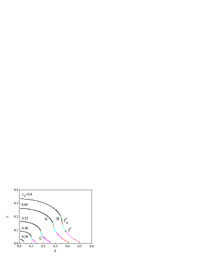
Figure 1: The plot of $T_{M}(\delta)$ for $\lambda_{M}=$ 0.28, 0.4, 0.52, 0.68, and 0.80, and $T_{M}^{*}$ and $T^{*}$. The unit of energy is $\omega_{c}$. ($\omega_{c}=1$). $T_{M}^{*}$ is the boundary between $q=0$ (C) and $q\neq 0$ (IC) SDW from solving Eq. (22). $T^{*}$ is the boundary between the phase separation and coexistence between SDW and SC determined by Eq. (36). For a given $\lambda_{M}$, in terms of the multicritical temperature $T_{c}$, the region of $T_{M}^{0}>T_{c}>T_{M}^{*}$ (black) corresponds to the phase separation between C-SDW and SC, $T_{M}^{*}>T_{c}>T^{*}$ (cyan) to the phase separation between IC-SDW and SC, and $T_{c}<T^{*}$ (pink) corresponds to the coexistence between IC-SDW and SC. As $\lambda_{M}$ is increased the region of the discontinuous thermodynamic transitions intervenes around $T_{M}^{*}$ and in the low temperature region as indicated by the green and red lines. The points marked by A, B, and C correspond to the representative cases of the phase separated C-SDW and SC, phase separated discontinuous C-SDW and SC, and coexisting IC-SDW and SC phases, respetively. The A, B, C cases are presented in more detail in Figs. 2, 3, and 4, respectively.

The nature of the transitions, that is, whether the magnetic and superconducting transitions are continuous or discontinuous, and whether $\Delta$ and $m$ coexist or not is determined by the 4th order terms. Expansion of the GL free energy of Eq. (II) up to the 4th order yields

$$F^{(4)}=\beta_{M}|m|^{4}+\beta_{\Delta}|\Delta|^{4}+\beta^{\prime}|m|^{2}|\Delta|^{2}.$$ (23)

All other combination terms vanish. The expressions of the coefficients are collected in the appendix. If all coefficients $\beta_{M}$, $\beta_{\Delta}$, $\beta^{\prime}$ are positive, then the magnetic and superconducting transitions as $T$ is reduced are continuous. Depending on the relations among the coefficients as will be discussed below, $m$ and $\Delta$ may coexist or repel each other as the doping is varied below $T_{c}$. The negative $\beta_{M}$, on the other hand, means discontinuous magnetic transition as $T$ is reduced. This occurs in the vicinity of the C-IC transition in the present model when $\lambda_{M}$ is large, as will be discussed below.

In order to determine the phase coexistence/separation we follow the standard statistical mechanics procedure and focus around the multicritical point where $T_{M}(\delta)=T_{c}$.Choi et al. (1989); Choi and Mele (1989) We write

$$\chi_{S}(T)-\lambda_{S}^{-1}=\frac{T-T_{c}}{T_{c}},$$ (24)

$$\chi_{M}(T)-\lambda_{M}^{-1}=A_{M}\frac{T-T_{c}}{T_{c}},$$ (25)

where $0<A_{M}<1$ is given by

$$A_{M}=T_{c}\ \frac{\partial\chi_{M}(\delta_{c},T_{c},q_{c})}{\partial T}$$

$$=\frac{1}{2}\left<\int_{-\omega_{c}}^{\omega_{c}}d\xi\frac{1}{\xi-q\cos\theta}\frac{\xi+\delta}{2T_{c}}{\rm sech}^{2}\left(\frac{\xi+\delta}{2T_{c}}\right)\right>_{\theta}.$$

We now introduce the field $\eta$ to make the 2nd order terms isotropic in the order parameter space.

$$\eta=\sqrt{A_{M}}\ m$$ (27)

and write

$$F^{(2)}=\frac{T-T_{c}}{T_{c}}\left(|\eta|^{2}+|\Delta|^{2}\right).$$ (28)

Collecting the 2nd and 4th order terms we have

$$F=\frac{T-T_{c}}{T_{c}}\left(|\eta|^{2}+|\Delta|^{2}\right)+a|\eta|^{4}+b|\Delta|^{4}+c|\eta|^{2}|\Delta|^{2},$$

where the coefficients are given by

$$a=\frac{\beta_{M}}{A_{M}^{2}},~{}~{}b=\beta_{\Delta},~{}~{}c=\frac{\beta^{\prime}}{A_{M}}.$$ (30)

The isotropic 2nd order terms suggest writing

$$|\eta|=r\cos\theta,~{}~{}|\Delta|=r\sin\theta.$$ (31)

The free energy can now be written as

$$F=$$

$$\frac{T-T_{c}}{T_{c}}\ r^{2}+r^{4}\left[a\cos^{4}\theta+b\sin^{4}\theta+c\cos^{2}\theta\sin^{2}\theta\right].$$

For

$$a+b-c>0,$$ (33)

the free energy takes the minimum with respect to $\theta$ when

$$\cos^{2}\theta=\beta,$$ (34)

where $\beta$ is given by

$$\beta=\frac{b-c/2}{a+b-c}.$$ (35)

We then have

$$m\neq 0,~{}\Delta=0,~{}~{}{\rm for} \beta\geq 1,$$

$$m=0,~{}\Delta\neq 0,~{}~{}{\rm for} \beta\leq 0,$$

$$m\neq 0,~{}\Delta\neq 0,~{}~{}{\rm for} 0<\beta<1.$$ (36)

Eq. (36), of course, represents the coexisting region. It may be rewritten in terms of $a,~{}b,~{}c$ as

$$a>c/2~{}{~{}\rm and~{}}~{}b>c/2.$$ (37)

Otherwise, the two orders phase separate and the first order phase transition shows up as $\delta$ changes below $T_{c}$. The coefficients $a,~{}b$, and $c$ can be calculated from Eqs. (23) and (30). Notice that the coexistence condition of Eq. (37) is more restrictive than the condition

$$ab>c^{2}/4$$ (38)

given by Vorontsov $et~{}al.$Vorontsov et al. (2010) The value of $\beta$ determines the ratio of the two condensates by Eq. (31) to give

$$\Delta^{2}=\frac{T_{c}-T}{2T_{c}}\frac{a-c/2}{ab-c^{2}/4},$$

$$m^{2}=\frac{1}{A_{M}^{2}}\frac{T_{c}-T}{2T_{c}}\frac{b-c/2}{ab-c^{2}/4}.$$ (39)

The GL expansion is only valid close to the multicritical point. As $T$ is lowered further below $T_{c}$, the order parameters become larger and we need next-order terms in the GL expansion to describe the critical phenomena with the same accuracy. This is very tedious and inefficient. We therefore obtain the order parameters $m$ and $\Delta$ self-consistently with numerical iterations as explained before. In the following section we will present the results.

III Results

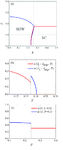
Figure 2: (a) The phase diagram of the SDW and SC for $\lambda_{M}=0.68$ and $\lambda_{S}=0.55$ where the tricritical point is at the point A on the second line from the top in the Fig. 1. It shows the phase separation between C-SDW and SC. (b) The SC order parameter $\Delta$ and SDW order parameter $m$ as a function of temperature at $\delta=\delta_{c}-\delta_{step}$ as indicated by the vertical dashed line in (a). (c) The order parameter $\Delta$ and $m$ as a function of $\delta$ at $T=0.1$ as indicated by the horizontal dashed line in (a).

To map out the phase boundary between the SDW and SC phases we first calculate $T_{M}(\delta)$ which is determined by $\lambda_{M}$ via Eq. (22). We considered the cases $\lambda_{M}=$ 0.28, 0.4, 0.52, 0.68, and 0.80 for representative values and corresponding $T_{M}(\delta)$ are shown in Fig. 1. The incommensurability $q$ was computed by maximizing $\chi_{M}$ of Eq (22) with respect to $q$ for given $T$ and $\delta$. $q=0$ and $\neq 0$ mean, respectively, the C-SDW and IC-SDW. The boundary between $q=0$ and $q\neq 0$ are marked on the $T_{M}(\delta)$ curves by $T_{M}^{*}$. We found

$$T_{M}^{*}=0.56\ T_{M}^{0}$$ (40)

in agreement with Ref. Vorontsov et al. (2009). This corresponds to

$$\frac{\delta}{2T_{M}^{*}}=0.958$$ (41)

which can be calculated from $\chi_{M}$ of Eq. (20) for $q=0$.

We also computed the anisotropy coefficient $\beta$ along $T_{M}(\delta)$ as the multicritical point is lowered along the curve. For a given $\lambda_{M}$, a smaller $\lambda_{S}$ means that the multicritical point where $T_{M}(\delta_{c})=T_{c}$ is at larger $\delta_{c}$ and smaller $T_{c}$. The computation of $\beta$ yields that there exists the critical $T^{*}$ such that $m$ and $\Delta$ phase separate for $T_{c}>T^{*}$ and coexist for $T_{c}<T^{*}$. We found

$$T^{*}=0.35\ T_{M}^{0}.$$ (42)

In Fig. 1, the black color of each $T_{M}(\delta)$ curve represents the phase separated C-SDW and SC where $T_{M}^{0}>T_{c}>T_{M}^{*}$, the cyan the phase separated IC-SDW and SC where $T_{M}^{*}>T_{c}>T^{*}$, and the pink represents the coexisting IC-SDW and SC phases where $T^{*}>T_{c}$. The coexisting SDW and SC are possible only for IC cases for the sign changed pairing in agreement with Ref. Vorontsov et al. (2009).

An interesting observation is made for large $\lambda_{M}$ such as $\lambda=0.8$ of Fig. 1. The coefficient $\beta_{M}$ of Eq. (48) of the 4th order SDW term becomes negative in the vicinity of the boundary between the C and IC-SDW. It means that the SDW transition as $T$ is reduced is discontinuous. See the discontinuous changes of the order parameters as the temperature is reduced as shown in Fig. 3(b). Incidentally, the thermodynamic first order SDW transition was not reported in the weak coupling calculation of Vorontsov $et~{}al$. Vorontsov et al. (2009) To check the discontinuous C-SDW transition as the mark B of Fig. 1 stands for, put $q=0$ in $\beta_{M}$ given by Eq. (48). Take the limit $\omega_{c}\rightarrow\infty$ and put $x=\xi/2T$ and $y=\delta/2T$.

$$\beta_{M}=\frac{1}{(2T)^{2}}\int_{-\infty}^{\infty}\frac{dx}{x^{3}}\left[\tanh\left(x+y\right)-x\ {\rm sech^{2}}\left(x+y\right)\right].$$ (43)

The integral changes sign at $y=0.955$ which means that for $\delta/2T_{M}>0.955$ the first order SDW transition occurs. Comparing this with the $\delta/2T_{M}^{*}=0.958$ of Eq. (41) means that the first order SDW transition intervenes near the C-SDW and IC-SDW boundary. The self-consistent numerical calculations indeed confirm this result as presented in Fig. 3. In our calculation it does not show up when $\lambda_{M}$ is small but begins to emerge when $\lambda_{M}\gtrsim 0.5$ probably because the discontinuity for small $\lambda_{M}$ is too small. As $\delta$ increases further, however, the nonzero $q$ increases the $\chi_{M}$, and IC second order transition preempts the first order transition as shown in Fig. 1.

Then we consider three cases where the points marked by A, B, and C on Fig. 1 are the multicritical point and calculated the phase diagram in the $T-\delta$ plane. The SDW and SC order parameters $m$ and $\Delta$ as a function of $T$ and $\delta$ are calculated by solving the gap equations via numerical iterations. The results like the phase separation/coexistence are fully consistent with the GL expansion. Let us first consider the point A. The computation of $\beta$ at the A point yields $\beta>1$ corresponding to the phase separation between C-SDW and SC. The phase transition line below $T_{c}$ was calculated with the numerical iterations of the gap equations of Eqs. (12) and (II). The results are shown in the Fig. 2. Fig. 2(b) and (c) present, respectively, the order parameters $\Delta$ and $m$ as functions of $T$ at $\delta=\delta_{0}-\delta_{step}$ and as functions of $\delta$ at $T=0.01$ as indicated by the dashed lines. $m$ shows the second order phase transition as a function of $T$, and the $\Delta$ and $m$ show the first order phase transition as functions of $\delta$ below $T_{c}$. This indicates that the SDW and SC orders phase separate as the doping is varied as was mentioned in the Introduction for the 1111 compounds. La1111,Luetkens et al. (2009) Sm1111,Drew et al. (2009) and Ce1111 compoundsZhao et al. (2008) all showed the phase separation as the doping was changed.

Now, let us turn to the case where the multicritical point is at the point B corresponding to $\lambda_{M}=0.80$ and $\lambda_{S}=0.55$. As alluded previously, the 4th order term of the GL expansion $\beta_{M}$ at the point B becomes negative in this case and the SDW transition as $T$ is reduced is discontinuous. The phase diagram in the $T-\delta$ plane obtained by the self-consistent numerical calculations of the gap equation is shown in Fig. 3(a). The temperature dependence of the order parameters $m$ and $\Delta$ is shown in (b). The $m$ exhibits the abrupt onset at $T=T_{M}$. The experiments were reported to be the continuous transitions for $m$ as a function of $T$.Luetkens et al. (2009) The transitions, however, could be equally well described as a weakly first order as shown in the present calculations. On the other hand, the abrupt change of $T_{M}$ and $T_{c}$ as a function of doping was not seen in the present model calculation. The experiments reported that the SDW (SC) showed up in the orthorhombic (tetragonal) phase which indicates the potential importance of the spin-lattice coupling. The discrepancy between the experiments and the present calculation could be due to the neglect of the spin-lattice coupling.

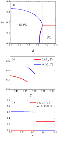
Figure 3: (a) The phase diagram of the SDW and SC for $\lambda_{M}=0.8$ and $\lambda_{S}=0.55$ corresponding to the point B in the Fig. 1. It exhibits the discontinuous change of transition temperatures between C-SDW and SC at the critical $\delta_{c}$. (b) The $\Delta$ and $m$ as a function of temperature at $\delta=\delta_{c}$ as indicated by the vertical dotted line in (a). (c) The order parameter $\Delta$ and $m$ as a function of $\delta$ at $T=0.1$ as indicated by the horizontal dotted line in (a).

Fig. 4 shows the case where the tetracritical point is at the point C corresponding to $\lambda_{M}=0.52$ and $\lambda_{S}=0.30$. $0<\beta<1$ is this case which means the IC-SDW and SC phases coexist microscopically, that is, both $m$ and $\Delta$ order parameters are nonzero at the same point in the real space. The phase diagram of Fig. 4(a) was obtained with the numerical iterations of the gap equations of (44), (45), and (46). The order parameters change continuously and the all the lines represent the second order transition. The green shaded region of Fig. 4 represents the parameter space where SDW and SC coexist microscopically. Figure (b) plots $m$ and $\Delta$ as functions of $T$ at $\delta=0.18$ indicated by the dotted vertical line in figure (a). Note that $m$ decreases as $T$ is lowered below the coexisting region because SC begins to partially gap out the Fermi surface. Figure (c) shows $m$ and $\Delta$ as functions of $\delta$ at $T=0.019$ indicated by the dotted horizontal line in the plot (a). The SDW and SC order coexist in the region of $0.16\lesssim\delta\lesssim 0.21$ in the low temperature limit. This result nicely corresponds to the Co doped 122 compounds. As was mentioned in the Introduction, Laplace $et~{}al.$Laplace et al. (2009) reported that the IC-SDW coexists with the SC on the atomic scale in Ba(Fe_1-xCo_x)₂As₂. This result was later confirmed by Julien $et~{}al$ on Ba(Fe_1-xCo_x)₂As₂Julien et al. (2009) and by Parker $et~{}al.$ on NaFe_1-xM_xAs (M=Co, Ni).Parker et al. (2010)

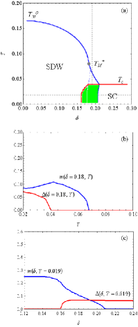
Figure 4: (a) The phase diagram obtained from the self-consistent numerical iterations of the gap equations for $\lambda_{M}=0.52,~{}\lambda_{S}=0.30.$ The tetracritical point corresponds to the point C in the Fig. 1. The green shade in fig(a) represents the coexisting region of IC-SDW and SC. The dashed line branching off from the $T_{M}^{*}$ represents the boundary between C and IC-SDW. In figures (b) and (c), the order parameters along the dotted lines of figure (a) are plotted. The red line is $\Delta$ and the blue line is $m$ as a function of temperature at $\delta=0.18$ and as a function of doping $T=0.019$, respectively. All transitions below $T_{c}$ are continuous. Note in figure (b) that $m$ decreases as $T$ is lowered below the coexisting region because SC begins to gap out the Fermi surface partially.

IV Conclusions

In this paper, we examined the interplay between the spin density wave and $\pi$ phase shifted superconductivity in the Fe pnictide superconductors. We have obtained the phase diagram in the plane of the temperature $T$ and chemical potential $\delta$ with the combination of the Ginzburg-Landau expansion of the free energy near the multicritical point and the self-consistent numerical iterations of the gap equations. By calculating the multicritical temperature $T_{c}$ as a function of the chemical potential $\delta$ as shown in Fig. 1, we presented possible cases of phase separation/coexistence among the commensurate SDW, incommensurate SDW, and superconducting phases.

Then three typical cases were considered in more detail. The phase separation of C-SDW and SC for $T_{c}>T_{M}^{*}$ was shown in Fig. 2. The phase diagram in the $T-\delta$ plane, the $T$ and $\delta$ dependences of the SDW and SC order parameters were shown. In Fig. 3, the discontinuous SDW–SC transition case was presented. And in Fig. 4, the coexisting IC-SDW and SC for $T_{c}<T^{*}$ case was presented.

In doing so, we employed a systematic way of determining the phase separation or coexistence between SDW and SC orders from the 4th order terms of the Ginzburg-Landau free energy expansion. We found that if $T_{c}$ is larger than $T^{*}$ then the two orders phase separate, but coexist for $T_{c}<T^{*}$ unless the first order transition intervenes. Although the SDW transitions as temperature is lowered are continuous for most of the parameter space, they can become first order if the doping at the multicritical point becomes large. Then the first order transition intervenes in between the C-SDW and IC-SDW boundary. This makes the phase boundaries more complicated than previously reported as presented in Fig. 1.

Finally, we remark that the shapes of the electron Fermi surfaces take quite different forms for different class of the pnictides. The effect of the FS shapes on the phase coexistence was studied in Ref. Vorontsov et al. (2010). Also, the effect of pairing symmetry on the phase separation/coexistence will be interesting. We are currently applying the present method to understand how the phase coexistence/separation phenomenon depends on the pairing symmetry.

Appendix A Incommensurate SDW

In the appendix, we collect the technical details of the Ginzburg-Landau expansion of the free energy for the incommensurate SDW cases. The energy of Eq. (15) above is generalized for the non-zero incommensurability ($q\neq 0$) to

$$E_{\pm}=\left\{\left[\sqrt{m^{2}+\left(\xi-q\cos\theta\right)^{2}}\pm\left(\delta+q\cos\theta\right)\right]^{2}+\Delta^{2}\right\}^{1/2},$$ (44)

and the SDW order parameter $m$ and superconducting order parameter $\Delta$ to

$$\Delta = \lambda_{S}\sum_{\sigma=\pm}\frac{1}{2}\left<\int_{-\omega_{c}}^{\omega_{c}}d\xi\frac{\Delta}{2E_{\sigma}}\tanh\left(\frac{E_{\sigma}}{2T}\right)\right>_{\theta},$$ (45)

$$m = \lambda_{M}\sum_{\sigma=\pm}\frac{1}{2}\left<\int_{-\omega_{c}}^{\omega_{c}}d\xi\frac{m}{2E_{\sigma}}\left(1+\frac{\sigma\left(\delta+q\cos\theta\right)}{\sqrt{\left(\xi-q\cos\theta\right)^{2}+m^{2}}}\right)\tanh\left(\frac{E_{\sigma}}{2T}\right)\right>_{\theta}.$$ (46)

The 4th order coefficients, $\beta_{\Delta}$, $\beta_{M}$, and $\beta^{\prime}$, of the Ginzburg–Landau expansion of the free energy around the multicritical point of Eq. (23) may be obtained by the derivative of the free energy of Eq. (II) with respect to the order parameters. They are given by

$$\beta_{\Delta}=\frac{1}{4}\int_{-\omega_{c}}^{\omega_{c}}d\xi\frac{1}{(\xi+\delta)^{3}}\left[\tanh\left(\frac{\xi+\delta}{2T}\right)-\frac{\xi+\delta}{2T}{\rm sech^{2}}\left(\frac{\xi+\delta}{2T}\right)\right],$$ (47)

$$\beta_{M}=\int_{-\omega_{c}}^{\omega_{c}}d\xi\left<\frac{1}{(\xi-q\cos\theta)^{3}}\left[\tanh\left(\frac{\xi+\delta}{2T}\right)-\frac{\xi-q\cos\theta}{2T}{\rm sech^{2}}\left(\frac{\xi+\delta}{2T}\right)\right]\right>_{\theta},$$ (48)

$$\beta^{\prime}=\frac{1}{4}\int_{-\omega_{c}}^{\omega_{c}}d\xi\left<\frac{1}{(\xi-q\cos\theta)(\xi+\delta)^{2}}\right>_{\theta}\left[\tanh\left(\frac{\xi+\delta}{2T}\right)-\frac{\xi+\delta}{2T}{\rm sech^{2}}\left(\frac{\xi+\delta}{2T}\right)\right].$$ (49)

The 4th order coefficients are then used to compute the anisotropy coefficient $\beta$ using the equations (II), (30), and (35). The $\beta$ determines the phase coexistence or separation by the condition of Eq. (36).

References

- Kamihara et al. (2008) Y. Kamihara, T. Watanabe, M. Hirano, and H. Hosono, J. Am. Chem. Soc. 130, 3296 (2008).
- Chen et al. (2008a) G. F. Chen, Z. Li, D. Wu, G. Li, W. Z. Hu, J. Dong, P. Zheng, J. L. Luo, and N. L. Wang, Phys. Rev. Lett. 100, 247002 (2008a).
- Chen et al. (2008b) X. H. Chen, T. Wu, G. Wu, R. H. Liu, H. Chen, and D. F. Fang, Nature 453, 761 (2008b).
- Fang et al. (2009) L. Fang, H. Luo, P. Cheng, Z. Wang, Y. Jia, G. Mu, B. Shen, I. I. Mazin, L. Shan, C. Ren, et al., arXiv:0903.2418 (2009).
- Christianson et al. (2008) A. D. Christianson, E. A. Goremychkin, R. Osborn, S.Rosenkranz, M. D. Lumsden, C. D. Malliakas, l. S. Todorov, H.Claus, D. Y. Chung, M. G. Kanatzidis, et al., Nature 456, 930 (2008).
- Uemura (2009) Y. J. Uemura, Nature Mat. 8, 253 (2009).
- Sanna et al. (2004) S. Sanna, G. Allodi, G. Concas, A. D. Hillier, and R. D. Renzi, Phys. Rev. Lett. 93, 207001 (2004).
- Knebel et al. (2009) G. Knebel, D. Aoki, J.-P. Brison, L. Howald, G. Lapertot, J. Panarin, S. Raymond, and J. Flouquet, Phys. Stat. Sol. (B) 247, 557 (2009).
- Park et al. (2006) T. Park, F. Ronning, H. Yuan, M. Salamon, R. Movshovich, J. Sarrao, and J. Thompson, Nature 440, 65 (2006).
- Yashima et al. (2009) M. Yashima, H. Mukuda, Y. Kitaoka, H. Shishido, R. Settai, and Y. Ōnuki, Phys. Rev. B 79, 214528 (2009).
- Luetkens et al. (2009) H. Luetkens, H. H. Klauss, M. Kraken, F. J. Litterst, T. Dellmann, R. Klingeler, C. Hess, R. Khasanov, A. Amato, C. Baines, et al., Nature Mat. 8, 305 (2009).
- Drew et al. (2009) A. J. Drew, C. Niedermayer, P. J. Baker, F. L. Pratt, S. J. Blundell, T. Lancaster, R. H. Liu, G. Wu, X. H. Chen, I. Watanabe, et al., Nature Mat. 8, 310 (2009).
- Zhao et al. (2008) J. Zhao, Q. Huang, C. de la Cruz, S. Li, J. W. Lynn, Y. Chen, M. A. Green, G. F. Chen, G. Li, Z. Li, et al., Nature Mat. 7, 953 (2008).
- Laplace et al. (2009) Y. Laplace, J. Bobroff, F. Rullier-Albenque, D. Colson, and A. Forget, Phys. Rev. B 80, 140501 (2009).
- Julien et al. (2009) M.-H. Julien, H. Mayaffre, M. Horvatic, C. Berthier, X. D. Zhang, W. Wu, G. F. Chen, N. L. Wang, and J. L. Luo, Europhys. Lett. 87, 37001 (2009).
- Parker et al. (2010) D. R. Parker, M. J. P. Smith, T. Lancaster, A. J. Steele, I. Franke, P. J. Baker, F. L. Pratt, M. J. Pitcher, S. J. Blundell, and S. J. Clarke, Phys. Rev. Lett. 104, 057007 (2010).
- Vorontsov et al. (2009) A. B. Vorontsov, M. G. Vavilov, and A. V. Chubukov, Phys. Rev. B 79, 060508 (2009).
- Vorontsov et al. (2010) A. B. Vorontsov, M. G. Vavilov, and A. V. Chubukov, Phys. Rev. B 81, 174538 (2010).
- Cvetkovic and Tesanovic (2009) V. Cvetkovic and Z. Tesanovic, Europhys. Lett. 85, 37002 (2009).
- Parker et al. (2009) D. Parker, M. G. Vavilov, A. V. Chubukov, and I. I. Mazin, Phys. Rev. B 80, 100508 (2009).
- Fernandes et al. (2010) R. M. Fernandes, D. K. Pratt, W. Tian, J. Zarestky, A. Kreyssig, S. Nandi, M. G. Kim, A. Thaler, N. Ni, P. C. Canfield, et al., Phys. Rev. B 81, 140501 (2010).
- Mazin et al. (2008) I. I. Mazin, D. J. Singh, M. D. Johannes, and M. H. Du, Phys. Rev. Lett. 101, 057003 (2008).
- Kuroki et al. (2008) K. Kuroki, S. Onari, H. Arita, Y. Tanaka, H. Kontani, and H. Aoki, Phys. Rev. Lett. 101, 087004 (2008).
- Bang and Choi (2008) Y. Bang and H.-Y. Choi, Phys. Rev. B 78, 134523 (2008).
- Lee and Choi (2009) H. C. Lee and H. Y. Choi, Journal of Physics: Condensed Matter 21, 445701 (2009).
- Negele and Orland (1988) J. W. Negele and H. Orland, Quantum Many-Particle Systems (Addison-Wesley, New York, 1988).
- Choi et al. (1989) H.-Y. Choi, A. B. Harris, and E. J. Mele, Phys. Rev. B 40, 3766 (1989).
- Choi and Mele (1989) H.-Y. Choi and E. J. Mele, Phys. Rev. B 40, 3439 (1989).