Heuristics in Conflict Resolution

Abstract

Modern solvers for Boolean Satisfiability (SAT) and Answer Set Programming (ASP) are based on sophisticated Boolean constraint solving techniques. In both areas, conflict-driven learning and related techniques constitute key features whose application is enabled by conflict analysis. Although various conflict analysis schemes have been proposed, implemented, and studied both theoretically and practically in the SAT area, the heuristic aspects involved in conflict analysis have not yet received much attention. Assuming a fixed conflict analysis scheme, we address the open question of how to identify “good” reasons for conflicts, and we investigate several heuristics for conflict analysis in ASP solving. To our knowledge, a systematic study like ours has not yet been performed in the SAT area, thus, it might be beneficial for both the field of ASP as well as the one of SAT solving.

Introduction

The popularity of Answer Set Programming (ASP; (?)) as a paradigm for knowledge representation and reasoning is mainly due to two factors: first, its rich modeling language and, second, the availability of high-performance ASP systems. In fact, modern ASP solvers, such as clasp (?), cmodels (?), and smodels${}_{\text{{cc}}}$ (?), have meanwhile closed the gap to Boolean Satisfiability (SAT; (?)) solvers. In both fields, conflict-driven learning and related techniques have led to significant performance boosts (?; ?; ?; ?). The basic prerequisite for the application of such techniques is conflict analysis, that is, the extraction of non-trivial reasons for dead ends encountered during search. Even though ASP and SAT solvers exploit different inference patterns, their underlying search techniques are closely related to each other. For instance, the basic search strategy of SAT solver chaff (?), nowadays a quasi standard in SAT solving, is also exploited by ASP solver clasp, in particular, the principles of conflict analysis are similar. Vice versa, the solution enumeration approach implemented in clasp (?) could also be applied by SAT solvers. Given these similarities, general search or, more specifically, conflict analysis techniques developed in one community can (almost) immediately be exploited in the other field too.

In this paper, we address the problem of identifying “good” reasons for conflicts to be recorded within an ASP solver. In fact, conflict-driven learning exhibits several degrees of freedom. For instance, several constraints may become violated simultaneously, in which case one can choose the conflict(s) to be analyzed. Furthermore, distinct schemes may be used for conflict analysis, such as the resolution-based First-UIP and Last-UIP scheme (?). Finally, if conflict analysis is based on resolution, several constraints may be suitable resolvents, likewise permitting to eliminate some literal in a resolution step.

For the feasibility of our study, it was necessary to prune dimensions of freedom in favor of predominant options. In the SAT area, the First-UIP scheme (?) has empirically been shown to yield better performance than other known conflict resolution strategies (?). We thus fix the conflict analysis strategy to conflict resolution according to the First-UIP scheme. Furthermore, it seems reasonable to analyze the first conflict detected by a solver (although conflicts encountered later on may actually yield “better” reasons). This leaves to us the choice of the resolvents to be used for conflict resolution, and we investigate this issue with respect to different goals: reducing the size of reasons to be recorded, skipping greater portions of the search space by backjumping (explained below), reducing the number of conflict resolution steps, and reducing the overall number of encountered conflicts (roughly corresponding to runtime). To this end, we modified the conflict analysis procedure of our ASP solver clasp for accommodating a variety of heuristics for choosing resolvents. The developed heuristics and comprehensive empirical results for them are presented in this paper.

Logical Background

We assume basic familiarity with answer set semantics (see, for instance, (?)). This section briefly introduces notations and recalls a constraint-based characterization of answer set semantics according to (?). We consider propositional (normal) logic programs over an alphabet $\mathcal{P}$. A logic program is a finite set of rules

$$p_{0}\leftarrow p_{1},\dots,p_{m},{\sim}{p_{m+1}},\dots,{\sim}{p_{n}}$$ (1)

where $0\leq m\leq n$ and $p_{i}\in\mathcal{P}$ is an atom for $0\leq i\leq n$. For a rule $r$ as in (1), let $head(r)=p_{0}$ be the head of $r$ and $body(r)=\{p_{1},\dots,p_{m},{\sim}{p_{m+1}},\dots,{\sim}{p_{n}}\}$ be the body of $r$. The set of atoms occurring in a logic program $\Pi$ is denoted by $atom(\Pi)$, and the set of bodies in $\Pi$ is $body(\Pi)=\{body(r)\mid r\in\Pi\}$. For regrouping bodies sharing the same head $p$, define $body(p)=\{body(r)\mid r\in\Pi,head(r)=p\}$.

For characterizing the answer sets of a program $\Pi$, we consider Boolean assignments $A$ over domain $\mathit{dom}(A)=atom(\Pi)\cup body(\Pi)$. Formally, an assignment $A$ is a sequence $(\sigma_{1},\ldots,\sigma_{n})$ of (signed) literals $\sigma_{i}$ of the form $\mathbf{T}v$ or $\mathbf{F}v$ for $v\in\mathit{dom}(A)$ and $1\leq i\leq n$. Intuitively, $\mathbf{T}v$ expresses that $v$ is true and $\mathbf{F}v$ that it is false in $A$. We denote the complement of a literal $\sigma$ by $\overline{\sigma}$, that is, $\overline{\mathbf{T}v}=\mathbf{F}v$ and $\overline{\mathbf{F}v}=\mathbf{T}v$. Furthermore, we let $A\circ B$ denote the sequence obtained by concatenating two assignments $A$ and $B$. We sometimes abuse notation and identify an assignment with the set of its contained literals. Given this, we access the true and false propositions in $A$ via $A^{\mathbf{T}}=\{p\in\mathit{dom}(A)\mid\mathbf{T}p\in A\}$ and $A^{\mathbf{F}}=\{p\in\mathit{dom}(A)\mid\mathbf{F}p\in A\}$. Finally, we denote the prefix of $A$ up to a literal $\sigma$ by

$$A[\sigma]=\left\{\begin{array}[]{@{}ll}(\sigma_{1},\dots,\sigma_{m})&\text{if }A=(\sigma_{1},\dots,\sigma_{m},\sigma,\dots,\sigma_{n})\\ A&\text{if }\sigma\notin A\ \text{.}\end{array}\right.$$

In our context, a nogood (?) is a set $\{\sigma_{1},\ldots,\sigma_{m}\}$ of literals, expressing a constraint violated by any assignment containing $\sigma_{1},\ldots,\sigma_{m}$. An assignment $A$ such that $A^{\mathbf{T}}\cup A^{\mathbf{F}}=\mathit{dom}(A)$ and $A^{\mathbf{T}}\cap A^{\mathbf{F}}=\emptyset$ is a solution for a set $\Delta$ of nogoods if $\delta\not\subseteq A$ for all $\delta\in\Delta$. Given a logic program $\Pi$, we below specify nogoods such that their solutions correspond to the answer sets of $\Pi$.

We start by describing nogoods capturing the models of the Clark’s completion (?) of a program $\Pi$. For $(\beta=\{p_{1},\dots,p_{m},{\sim}{p_{m+1}},\dots,{\sim}{p_{n}}\})\in\mathit{body}(\Pi)$, let

$$\Delta_{\beta}=\left\{\begin{array}[]{@{}l@{}}\\[-8.53581pt] \{\mathbf{T}p_{1},\dots,\mathbf{T}p_{m},\mathbf{F}p_{m+1},\dots,\mathbf{F}p_{n},\mathbf{F}\beta\},{}\\ \{\mathbf{F}p_{1},\mathbf{T}\beta\},\dots,\{\mathbf{F}p_{m},\mathbf{T}\beta\},{}\\ \{\mathbf{T}p_{m+1},\mathbf{T}\beta\},\dots,\{\mathbf{T}p_{n},\mathbf{T}\beta\}\\[1.42262pt] \end{array}\right\}\text{.}$$

Observe that every solution for $\Delta_{\beta}$ must assign body $\beta$ equivalent to the conjunction of its elements. Similarly, for an atom $p\in\mathit{atom}(\Pi)$, the following nogoods stipulate $p$ to be equivalent to the disjunction of $\mathit{body}(p)=\{\beta_{1},\dots,\beta_{k}\}$:

$$\Delta_{p}=\left\{\begin{array}[]{@{}l@{}}\\[-8.53581pt] \{\mathbf{F}\beta_{1},\dots,\mathbf{F}\beta_{k},\mathbf{T}p\},{}\\ \{\mathbf{T}\beta_{1},\mathbf{F}p\},\dots,\{\mathbf{T}\beta_{k},\mathbf{F}p\}\\[1.42262pt] \end{array}\right\}\text{.}$$

Combining the above nogoods for $\Pi$, we get

$$\Delta_{\Pi}=\mbox{$\bigcup$}_{\beta\in\mathit{body}(\Pi)}\Delta_{\beta}\cup\mbox{$\bigcup$}_{p\in\mathit{atom}(\Pi)}\Delta_{p}\text{ .}$$

The solutions for $\Delta_{\Pi}$ correspond one-to-one to the models of the completion of $\Pi$. If $\Pi$ is tight (?; ?), these models are guaranteed to match the answer sets of $\Pi$. This can be formally stated as follows.

Theorem 1 ((?))

Let $\Pi$ be a tight logic program. Then, $X\subseteq\mathit{atom}(\Pi)$ is an answer set of $\Pi$ iff $X=A^{\mathbf{T}}\cap\mathit{atom}(\Pi)$ for a (unique) solution $A$ for $\Delta_{\Pi}$.

We proceed by considering non-tight programs $\Pi$. As shown in (?), loop formulas can be added to the completion of $\Pi$ to establish full correspondence to the answer sets of $\Pi$. For $U\subseteq\mathit{atom}(\Pi)$, let $\mathit{EB}_{\Pi}(U)$ be

$$\{\mathit{body}(r)\mid r\in\Pi,\mathit{head}(r)\in U,\mathit{body}(r)\cap U=\emptyset\}\ \text{.}$$

Observe that $\mathit{EB}_{\Pi}(U)$ contains the bodies of all rules in $\Pi$ that can externally support (?) an atom in $U$. Given $U=\{p_{1},\dots,p_{j}\}$ and $\mathit{EB}_{\Pi}(U)=\{\beta_{1},\dots,\beta_{k}\}$, the following nogoods capture the loop formula of $U$:

$$\Lambda_{U}=\left\{\begin{array}[]{@{}l@{}}\\[-8.53581pt] \{\mathbf{F}\beta_{1},\dots,\mathbf{F}\beta_{k},\mathbf{T}p_{1}\},\dots,{}\\ \{\mathbf{F}\beta_{1},\dots,\mathbf{F}\beta_{k},\mathbf{T}p_{j}\}\\[1.42262pt] \end{array}\right\}\text{.}$$

Furthermore, we define

$$\Lambda_{\Pi}=\mbox{$\bigcup$}_{U\subseteq\mathit{atom}(\Pi)}\Lambda_{U}\text{ .}$$

By augmenting $\Delta_{\Pi}$ with $\Lambda_{\Pi}$, Theorem 1 can be extended to non-tight programs.

Theorem 2 ((?))

Let $\Pi$ be a logic program. Then, $X\subseteq\mathit{atom}(\Pi)$ is an answer set of $\Pi$ iff $X=A^{\mathbf{T}}\cap\mathit{atom}(\Pi)$ for a (unique) solution $A$ for $\Delta_{\Pi}\cup\Lambda_{\Pi}$.

By virtue of Theorem 2, the nogoods in $\Delta_{\Pi}\cup\Lambda_{\Pi}$ provide us with a constraint-based characterization of the answer sets of $\Pi$. However, it is important to note that the size of $\Delta_{\Pi}$ is linear in $\mathit{atom}(\Pi){\times}\mathit{body}(\Pi)$, while $\Lambda_{\Pi}$ contains exponentially many nogoods. As shown in (?), under current assumptions in complexity theory, the exponential number of elements in $\Lambda_{\Pi}$ is inherent, that is, it cannot be reduced significantly in the worst case. Hence, ASP solvers do not determine the nogoods in $\Lambda_{\Pi}$ a priori, but include mechanisms to determine them on demand. This is illustrated further in the next section.

Algorithmic Background

This section recalls the basic decision procedure of clasp (?), abstracting Conflict-Driven Clause Learning (CDCL; (?)) for SAT solving from clauses, that is, Conflict-Driven Nogood Learning (CDNL).

Conflict-Driven Nogood Learning

Algorithm 1 shows our main procedure for deciding whether a program $\Pi$ has some answer set. The algorithm starts with an empty assignment $A$ and an empty set $\nabla$ of recorded nogoods (Lines 1–2). Note that dynamic nogoods added to $\nabla$ in Line 5 are elements of $\Lambda_{\Pi}$, while those added in Line 9 result from conflict analysis (Line 8). In addition to conflict-driven learning, the procedure performs backjumping (Lines 10–11), guided by a decision level $k$ determined by conflict analysis. Via decision level $\mathit{dl}$, we count decision literals, that is, literals in $A$ that have been heuristically selected in Line 15. The initial value of $\mathit{dl}$ is $0$ (Line 3), and it is incremented in Line 16 before a decision literal is added to $A$ (Line 17). All literals in $A$ that are not decision literals have been derived by propagation in Line 5, and we call them implied literals. For any literal $\sigma$ in $A$, we write $\mathit{dl}(\sigma)$ to refer to the decision level of $\sigma$, that is, the value $\mathit{dl}$ had when $\sigma$ was added to $A$. After propagation, the main loop (Lines 4–17) distinguishes three cases: a conflict detected via a violated nogood (Lines 6–11), a solution (Lines 12–13), or a heuristic selection with respect to a partial assignment (Lines 14–17). Finally, note that a conflict at decision level $0$ signals that $\Pi$ has no answer set (Line 7).

Input : A program $\Pi$.

Output : An answer set of $\Pi$.

$A\leftarrow\emptyset$ // assignment over $\mathit{atom}(\Pi)\cup\mathit{body}(\Pi)$

$\nabla\leftarrow\emptyset$ // set of (dynamic) nogoods

$\mathit{dl}\leftarrow 0$ // decision level

loop   $(A,\nabla)\leftarrow\textnormal{{Propagation(}}\textnormal{\emph{$\Pi,\nabla,A$}}\textnormal{{)}}$

if $\varepsilon\subseteq A\textnormal{ for some }\varepsilon\in\Delta_{\Pi}\cup\nabla$ then  if $\mathit{dl}=0$ then return no answer set

$(\delta,k)\leftarrow\textnormal{{ConflictAnalysis(}}\textnormal{\emph{$\varepsilon,\Pi,\nabla,A$}}\textnormal{{)}}$

$\nabla\leftarrow\nabla\cup\{\delta\}$

$A\leftarrow A\setminus\{\sigma\in A\mid k<\mathit{dl}(\sigma)\}$

$\mathit{dl}\leftarrow k$ else if $A^{\mathbf{T}}\cup A^{\mathbf{F}}=\mathit{atom}(\Pi)\cup\mathit{body}(\Pi)$ then  return $A^{\mathbf{T}}\cap\mathit{atom}(\Pi)$ else  $\sigma_{d}\leftarrow\textnormal{{Select(}}\textnormal{\emph{$\Pi,\nabla,A$}}\textnormal{{)}}$

$\mathit{dl}\leftarrow\mathit{dl}+1$

$A\leftarrow A\circ(\sigma_{d})$    

Algorithm 1 CDNL

11

11

11

11

11

11

11

11

11

11

11

Propagation

Our propagation procedure, shown in Algorithm 2, derives implied literals and adds them to $A$. Lines 3–9 describe unit propagation (cf. (?)) on $\Delta_{\Pi}\cup\nabla$. If a conflict is detected in Line 4, unit propagation terminates immediately (Line 5). Otherwise, in Line 6, we determine all nogoods $\delta$ that are unit-resulting wrt $A$, that is, the complement $\overline{\sigma}$ of some literal $\sigma\in\delta$ must be added to $A$ because all other literals of $\delta$ are already true in $A$. If there is some unit-resulting nogood $\delta$ (Line 7), $A$ is augmented with $\overline{\sigma}$ in Line 8. Observe that $\delta$ is chosen non-deterministically, and several distinct nogoods may imply $\overline{\sigma}$ wrt $A$. This non-determinism gives rise to our study of heuristics for conflict resolution, selecting a resolvent among the nogoods $\delta$ that imply $\overline{\sigma}$.

The second part of Algorithm 2 (Lines 10–14) checks for unit-resulting or violated nogoods in $\Lambda_{\Pi}$. If $\Pi$ is tight (Line 10), sophisticated checks are unnecessary (cf. Theorem 1). Otherwise, we consider sets $U\subseteq\mathit{atom}(\Pi)$ such that $\mathit{EB}_{\Pi}(U)\subseteq A^{\mathbf{F}}$, called unfounded sets (?). An unfounded set $U$ is determined in Line 12 by a dedicated algorithm, where $U\cap A^{\mathbf{F}}=\emptyset$. If such a nonempty unfounded set $U$ exists, each nogood $\delta\in\Lambda_{U}$ is either unit-resulting or violated wrt $A$, and an arbitrary $\delta\in\Lambda_{U}$ is recorded in Line 14 for triggering unit propagation. Note that all atoms in $U$ must be falsified before another unfounded set is determined (cf. Lines 11–12). Eventually, propagation terminates in Line 13 if no nonempty unfounded set has been detected in Line 12.

Input : A program $\Pi$, a set $\nabla$ of nogoods, and an assignment $A$.

Output : An extended assignment and set of nogoods.

$U\leftarrow\emptyset$ // unfounded set

loop   repeat  if $\delta\subseteq A\textnormal{ for some }\delta\in\Delta_{\Pi}\cup\nabla$ then  return $(A,\nabla)$

  $\Sigma\leftarrow\{\delta\in\Delta_{\Pi}\cup\nabla\mid\delta\setminus A=\{\sigma\},\overline{\sigma}\notin A\}$

if $\Sigma\neq\emptyset$ then let $\sigma\in\delta\setminus A\textnormal{ for some }\delta\in\Sigma$ in  $A\leftarrow A\circ(\overline{\sigma})$   until $\Sigma=\emptyset$

if $\textsc{Tight}(\Pi)$ then return $(A,\nabla)$

$U\leftarrow U\setminus A^{\mathbf{F}}$

if $U=\emptyset$ then $U\leftarrow\textnormal{{UnfoundedSet(}}\textnormal{\emph{$\Pi,A$}}\textnormal{{)}}$

if $U=\emptyset$ then return $(A,\nabla)$

let $\delta\in\Lambda_{U}$ in $\nabla\leftarrow\nabla\cup\{\delta\}$

 

Algorithm 2 Propagation

10

10

10

10

10

10

10

10

10

10

Input : A violated nogood $\delta$, a program $\Pi$, a set $\nabla$ of nogoods, and an assignment $A$.

Output : A derived nogood and a decision level.

loop   let $\sigma\in\delta$ such that $\delta\setminus A[\sigma]=\{\sigma\}$

$k\leftarrow\mathit{max}(\{\mathit{dl}(\rho)\mid\rho\in\delta\setminus\{\sigma\}\}\cup\{0\})$

if $k=\mathit{dl}(\sigma)$ then  $\Sigma\leftarrow\{\varepsilon\in\Delta_{\Pi}\cup\nabla\mid\varepsilon\setminus A[\sigma]=\{\overline{\sigma}\}\}$

$\varepsilon\leftarrow\textnormal{{SelectAntecedent(}}\textnormal{\emph{$\Sigma$}}\textnormal{{)}}$

$\delta\leftarrow(\delta\setminus\{\sigma\})\cup(\varepsilon\setminus\{\overline{\sigma}\})$ else return $(\delta,k)$  

Algorithm 3 ConflictAnalysis

4

4

4

4

Conflict Analysis

Algorithm 3 shows our conflict analysis procedure, which is based on resolution. Given a nogood $\delta$ that is violated wrt $A$, we determine in Line 2 the literal $\sigma\in\delta$ added last to $A$. If $\sigma$ is the single literal of its decision level $\mathit{dl}(\sigma)$ in $\delta$ (cf. Line 3), it is called a unique implication point (UIP; (?)). Among a number of conflict resolution schemes, the First-UIP scheme, stopping conflict resolution as soon as the first UIP is reached, has turned out to be the most efficient and most robust strategy (?). Our conflict analysis procedure follows the First-UIP scheme by performing conflict resolution only if $\sigma$ is not a UIP (tested in Line 4) and, otherwise, returning $\delta$ along with the smallest decision level $k$ at which $\overline{\sigma}$ is implied by $\delta$ after backjumping (Line 8).

Let us take a closer look at conflict resolution steps in Lines 5–7. It is important to note that, if $\sigma$ is not a UIP, it cannot be the decision literal of $\mathit{dl}(\sigma)$. Rather, it must have been implied by some nogood $\varepsilon\in\Delta_{\Pi}\cup\nabla$. As a consequence, the set $\Sigma$ determined in Line 5 cannot be empty, and we call its elements antecedents of $\sigma$. Note that each antecedent $\varepsilon$ contains $\overline{\sigma}$ and had been unit-resulting immediately before $\sigma$ was added to $A$; we thus call $\varepsilon\setminus\{\overline{\sigma}\}$ a reason for $\sigma$. Knowing that $\sigma$ may have more than one antecedent, a non-deterministic choice among them is made in Line 6. Exactly this choice is subject to the heuristics studied below. Furthermore, as $\sigma$ is the literal of $\delta$ added last to $A$, $\delta\setminus\{\sigma\}$ is also a reason for $\overline{\sigma}$. Since they imply complementary literals, no solution can jointly contain both reasons, viz., $\delta\setminus\{\sigma\}$ and $\varepsilon\setminus\{\overline{\sigma}\}$. Hence, combining them in Line 7 gives again a nogood violated wrt $A$. Finally, note that conflict resolution is guaranteed to terminate at some UIP, but different heuristic choices in Line 6 may result in different UIPs.

Implication Graphs and Conflict Graphs

To portray the matter of choosing among several distinct antecedents, we modify the notion of an implication graph (?). At a given state of CDNL, the implication graph contains a node for each literal $\sigma$ in assignment $A$ and, for a violated nogood $\delta\subseteq A$, a node $\overline{\sigma}$ is included, where $\sigma$ is the literal of $\delta$ added last to $A$, that is, $\delta\setminus A[\sigma]=\{\sigma\}$. Furthermore, for each antecedent $\delta$ of an implied literal $\sigma$, the implication graph contains directed edges labeled with $\delta$ from all literals in the reason $\delta\setminus\{\overline{\sigma}\}$ to $\sigma$. Different from (?), where implication graphs reflect exactly one reason per implied literal, our implication graph thus includes all of them. If the implication graph contains both $\sigma$ and $\overline{\sigma}$, we call them conflicting literals. Note that an implication graph contains at most one such pair $\{\sigma,\overline{\sigma}\}$, called conflicting assignment, because our propagation procedure in Algorithm 2 stops as soon as a nogood becomes violated (cf. Lines 4–5).

An exemplary implication graph is shown in Figure 1. Each of its nodes (except for one among the two conflicting literals) corresponds to a literal that is true in assignment

$$A=\big{(}\mathbf{F}a,\mathbf{F}b,\underline{\mathbf{F}p},\underline{\mathbf{T}q},\underline{\mathbf{T}r},\mathbf{T}s,\mathbf{F}v,\mathbf{T}t,\mathbf{F}u,\mathbf{F}w,\mathbf{T}x\big{)}\ \text{.}$$

The three decision literals in $A$ are underlined, and all other literals are implied. For each literal $\sigma$, its decision level $\mathit{dl}(\sigma)$ is also provided in Figure 1 in parentheses. Every edge is labeled with at least one antecedent of its target, that is, the edges represent the following nogoods:

$$n_{0} =\{\mathbf{F}a,\mathbf{T}b\} n_{1} =\{\mathbf{T}r,\mathbf{F}s\}$$

$$n_{2} =\{\mathbf{T}s,\mathbf{F}t\} n_{3} =\{\mathbf{T}s,\mathbf{T}u\}$$

$$n_{4} =\{\mathbf{T}s,\mathbf{T}w\} n_{5} =\{\mathbf{T}r,\mathbf{T}v\}$$

$$n_{6} =\{\mathbf{T}q,\mathbf{F}v,\mathbf{T}w\} n_{7} =\{\mathbf{T}t,\mathbf{F}u,\mathbf{F}x\}$$

$$n_{8} =\{\mathbf{F}p,\mathbf{T}t,\mathbf{F}x\} n_{9} =\{\mathbf{F}w,\mathbf{T}x\}\ \text{.}$$

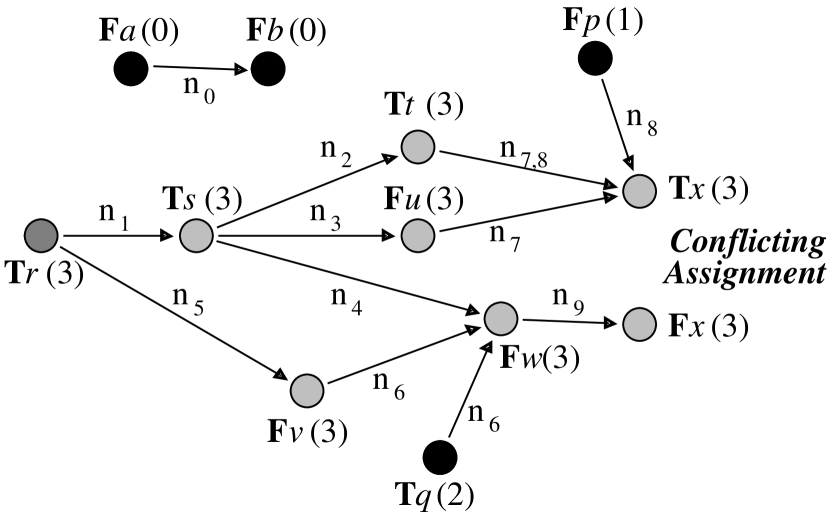
Figure 1: An exemplary implication graph containing a conflicting assignment.

Furthermore, nogood $\{\mathbf{T}a\}$ is unit-resulting wrt the empty assignment, thus, implied literal $\mathbf{F}a$ (whose decision level is $0$) does not have any incoming edge. Observe that the implication graph contains conflicting assignment $\{\mathbf{T}x,\mathbf{F}x\}$, where $\mathbf{T}x$ has been implied by nogood $n_{7}$ and likewise by $n_{8}$. It is also the last literal in $A$ belonging to violated nogood $n_{9}$, so that its complement $\mathbf{F}x$ is the second conflicting literal in the implication graph. Besides $\mathbf{T}x$, literal $\mathbf{F}w$ has multiple antecedents, namely, $n_{4}$ and $n_{6}$, which can be read off the labels of the incoming edges of $\mathbf{F}w$.

The conflict resolution done in Algorithm 3, in particular, the heuristic choice of antecedents in Line 6, can now be viewed as an iterative projection of the implication graph. In fact, if an implied literal has incoming edges with distinct labels, all edges with a particular label are taken into account, while the edges with different labels only are dropped. This observation motivates the following definition: a subgraph of an implication graph is a conflict graph if it contains a conflicting assignment and, for each implied literal $\sigma$ in the subgraph, the set of predecessors of $\sigma$ is a reason for $\sigma$. Note that this definition allows us to drop all literals that do not have a path to any conflicting literal, such as $\mathbf{F}a$ and $\mathbf{F}b$ in Figure 1. Furthermore, the requirement that the predecessors of an implied literal form a reason corresponds to the selection of an antecedent, where only the incoming edges with a particular label are traced via conflict resolution.

The next definition accounts for a particularity of ASP solving related to unfounded set handling: a conflict graph is level-aware if each conflicting literal $\sigma$ has some predecessor $\rho$ such that $\mathit{dl}(\rho)=\mathit{dl}(\sigma)$. In fact, propagation in Algorithm 2 is limited to falsifying unfounded atoms, thus, unit propagation on nogoods in $\Lambda_{\Pi}$ is performed only partially and may miss implied literals corresponding to external bodies (cf. (?)). If a conflict graph is not level-aware, the violated nogood $\delta$ provided as input to Algorithm 3 already contains a UIP, thus, $\delta$ itself is returned without performing any conflict resolution in-between. Given that we are interested in conflict resolution, we below consider level-aware conflict graphs only.

Finally, we characterize nogoods derived by Algorithm 3 by cuts in conflict graphs (cf. (?; ?)). A conflict cut in a conflict graph is a bipartition of the nodes such that all decision literals belong to one side, called reason side, and the conflicting assignment is contained in the other side, called conflict side. The set of nodes on the reason side that have some edge into the conflict side form the conflict nogood associated with a particular conflict cut. For illustration, a First-New-Cut (?) is shown in Figure 2. For the underlying conflict graph, we can choose among the incoming edges of $\mathbf{T}x$ whether to include the edges labeled with $n_{7}$ or the ones labeled with $n_{8}$. With $n_{7}$, we get conflict nogood $\{\mathbf{T}t,\mathbf{F}u,\mathbf{F}w\}$, while $n_{8}$ yields $\{\mathbf{F}p,\mathbf{T}t,\mathbf{F}w\}$.

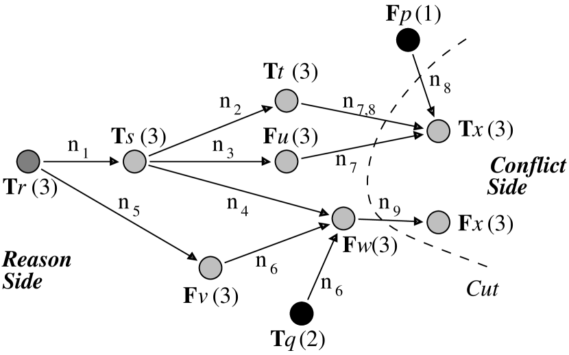
Figure 2: The implication graph with a First-New-Cut.

Different conflict cuts correspond to different resolution schemes, where we are particularly interested in the First-UIP scheme. Given a conflict graph and conflicting assignment $\{\sigma,\overline{\sigma}\}$, a UIP $\sigma_{\mathit{UIP}}$ can be identified as a node such that all paths from $\sigma_{d}$, the decision literal of decision level $\mathit{dl}(\sigma)=\mathit{dl}(\overline{\sigma})$, to either $\sigma$ or $\overline{\sigma}$ go through $\sigma_{\mathit{UIP}}$ (cf. (?)). In view of this alternative definition of a UIP, it becomes even more obvious than before that $\sigma_{d}$ is indeed a UIP, also called the Last-UIP. In contrast, a literal $\sigma_{\mathit{UIP}}$ is the First-UIP if it is the UIP “closest” to the conflicting literals, that is, if no other UIP is reachable from $\sigma_{\mathit{UIP}}$. The First-UIP-Cut is then given by the conflict cut that has all literals lying on some path from the First-UIP to a conflicting literal, except for the First-UIP itself, on the conflict side and all other literals (including the First-UIP) on the reason side. The First-UIP-Nogood, that is, the conflict nogood associated with the First-UIP-Cut, is exactly the nogood derived by conflict resolution in Algorithm 3 when antecedents that contribute edges to the conflict graph are selected for conflict resolution. Also note that the First-UIP-Cut for a conflict graph is unique, thus, by projecting an implication graph to a conflict graph, we implicitly fix the First-UIP-Nogood. With this is mind, the next section deals with heuristics for extracting conflict graphs from implication graphs.

Heuristics

In this section, we propose several heuristics for conflict resolution striving for different goals.

Recording Short Nogoods

Under the assumption that short nogoods prune larger portions of the search space than longer ones, a First-UIP-Nogood looks the more attractive the less literals it contains. In addition, unit propagation on shorter nogoods is usually faster and might even be enabled to use particularly optimized data structures, for instance, specialized to binary or ternary nogoods (?). As noticed in (?), a conflict nogood stays short when the resolvents are short, when the number of resolvents is small, or when the resolvents have many literals in common. In the SAT area, it has been observed that preferring short nogoods in conflict resolution may lead to resolution sequences involving mostly binary and ternary nogoods, so that derived conflict nogoods are not much longer than the originally violated nogoods (?). Our first heuristics, $H_{\mathit{short}}$, thus selects an antecedent containing the smallest number of literals among the available antecedents of a literal. Given the same implication graph as in Figure 1 and 2, $H_{\mathit{short}}$ may yield the conflict graph shown in Figure 3 by preferring antecedent $n_{7}$ of $\mathbf{T}x$ over $n_{8}$ and antecedent $n_{4}$ of $\mathbf{F}w$ over $n_{6}$ during conflict resolution. The corresponding First-UIP-Nogood, $\{\mathbf{T}s\}$, is indeed short and enables CDNL to after backjumping derive $\mathbf{F}s$ by unit propagation at decision level $0$. However, the antecedents $n_{7}$ and $n_{8}$ of $\mathbf{T}x$ are of the same size, thus, $H_{\mathit{short}}$ may likewise pick $n_{8}$, in which case the First-UIP-Cut in Figure 4 is obtained. The corresponding First-UIP-Nogood, $\{\mathbf{F}p,\mathbf{T}s\}$, is longer. Nonetheless, our experiments below empirically confirm that $H_{\mathit{short}}$ tends to reduce the size of First-UIP-Nogoods. But before, we describe further heuristics focusing also on other aspects.

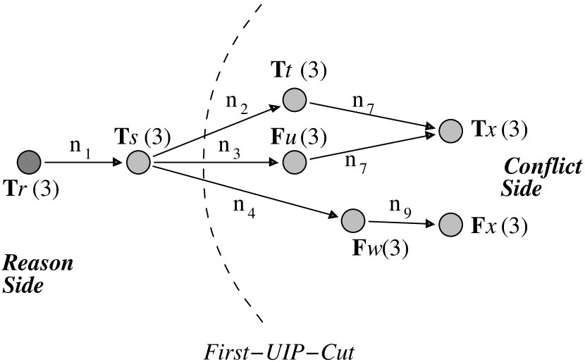
Figure 3: A First-UIP-Cut obtained with $H_{\mathit{short}}$.

Performing Long Backjumps

By backjumping, CDNL may skip the exhaustive exploration of regions of the search space, possibly escaping spare regions not containing any solution. Thus, it seems reasonable to aim at First-UIP-Nogoods such that their literals belong to small decision levels, as they are the determining factor for the lengths of backjumps. Our second heuristics, $H_{\mathit{lex}}$, thus uses a lexicographic order to rank antecedents according to the decision levels of their literals. Given an antecedent $\delta$ of a literal $\sigma$, we arrange the literals in the reason $\delta\setminus\{\overline{\sigma}\}$ for $\sigma$ in descending order of their decision levels. The so obtained sequence $(\sigma_{1},\dots,\sigma_{m})$, where $\delta\setminus\{\overline{\sigma}\}=\{\sigma_{1},\dots,\sigma_{m}\}$, induces a descending list $\mathit{levels}(\delta)=(\mathit{dl}(\sigma_{1}),\dots,\mathit{dl}(\sigma_{m}))$ of decision levels. An antecedent $\delta$ is then considered to be smaller than another antecedent $\varepsilon$, viz., $\delta<\varepsilon$, if the first element that differs in $\mathit{levels}(\delta)$ and $\mathit{levels}(\varepsilon)$ is smaller in $\mathit{levels}(\delta)$ or if $\mathit{levels}(\delta)$ is a prefix of $\mathit{levels}(\varepsilon)$ and shorter than $\mathit{levels}(\varepsilon)$. Due to the last condition, $H_{\mathit{lex}}$ also prefers an antecedent $\delta$ that is shorter than $\varepsilon$, provided that literals of the same decision levels as in $\delta$ are also found in $\varepsilon$. Reconsidering the implication graph in Figure 1 and 2, we obtain $\mathit{levels}(n_{8})=(3,1)<(3,3)=\mathit{levels}(n_{7})$ for antecedents $n_{7}$ and $n_{8}$ of $\mathbf{T}x$, and we have $\mathit{levels}(n_{4})=(3)<(3,2)=\mathit{levels}(n_{6})$ for antecedents $n_{4}$ and $n_{6}$ of $\mathbf{F}w$. By selecting antecedents that are lexicographically smallest, $H_{\mathit{lex}}$ leads us to the conflict graph shown in Figure 4. In this example, the corresponding First-UIP-Nogood, $\{\mathbf{F}p,\mathbf{T}s\}$, is weaker than $\{\mathbf{T}s\}$, which may be obtained with $H_{\mathit{short}}$ (cf. Figure 3).

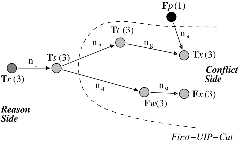
Figure 4: A First-UIP-Cut obtained with $H_{\mathit{lex}}$.

Given that lexicographic comparisons are computationally expensive, we also consider a lightweight variant of ranking antecedents according to decision levels. Our third heuristics, $H_{\mathit{avg}}$, prefers an antecedent $\delta$ over $\varepsilon$ if the average of $\mathit{levels}(\delta)$ is smaller than the average of $\mathit{levels}(\varepsilon)$. In our example, we get $\mathit{avg}[\mathit{levels}(n_{8})]=\mathit{avg}(3,1)=2<3=\mathit{avg}(3,3)=\mathit{avg}[\mathit{levels}(n_{7})]$ and $\mathit{avg}[\mathit{levels}(n_{6})]=\mathit{avg}(3,2)=2.5<3=\mathit{avg}(3)=\mathit{avg}[\mathit{levels}(n_{4})]$, yielding the conflict graph shown in Figure 5. Unfortunately, the corresponding First-UIP-Nogood, $\{\mathbf{F}p,\mathbf{T}q,\mathbf{T}r\}$, does not match the goal of $H_{\mathit{avg}}$ as backjumping only returns to decision level $2$, where $\mathbf{T}r$ is then flipped to $\mathbf{F}r$. Note that this behavior is similar to chronological backtracking, which can be regarded as the most trivial form of backjumping.

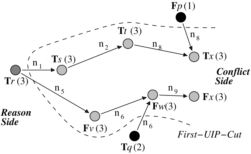
Figure 5: A First-UIP-Cut obtained with $H_{\mathit{avg}}$.

Shortening Conflict Resolution

Our fourth heuristics, $H_{\mathit{res}}$, aims at speeding up conflict resolution itself by shortening resolution sequences. In order to earlier encounter a UIP, $H_{\mathit{res}}$ prefers antecedents such that the number of literals at the current decision level $\mathit{dl}$ is smallest. In our running example, $H_{\mathit{res}}$ prefers $n_{8}$ over $n_{7}$ as it contains fewer literals whose decision level is $3$. However, antecedents $n_{4}$ and $n_{6}$ of $\mathbf{F}w$ are indifferent, thus, $H_{\mathit{res}}$ may yield either one of the conflict graphs in Figure 4 and 5.

Search Space Pruning

The heuristics presented above rank antecedents merely by structural properties, thus disregarding their contribution in the past to solving the actual problem. The latter is estimated by nogood deletion heuristics of SAT solvers (?; ?), and clasp also maintains activity scores for nogoods (?). Our fifth heuristics, $H_{\mathit{active}}$, makes use of them and ranks antecedents according to their activities.

Finally, we investigate a heuristics, $H_{\mathit{prop}}$, that stores (and prefers) the smallest decision level at which a nogood has ever been unit-resulting. The intuition underlying $H_{\mathit{prop}}$ is that the number of implied literals at small decision levels can be viewed as a measure for the progress of CDNL, in particular, as attesting unsatisfiability requires a conflict at decision level $0$. Thus, it might be a good idea to prefer nogoods that gave rise to implications at small decision levels.

Experiments

For their empirical assessment, we have implemented the heuristics proposed above in a prototypical extension of our ASP solver clasp version 1.0.2. (Even though there are newer versions of clasp, a common testbed, omitting some optimizations, is sufficient for a representative comparison.) Note that clasp (?) incorporates various advanced Boolean constraint solving techniques, e.g.:

• lookback-based decision heuristics (?),

• restart and nogood deletion policies (?),

• watched literals for unit propagation on “long” nogoods (?),

• dedicated treatment of binary and ternary nogoods (?), and

• early conflict detection (?).

Due to this variety, the solving process of clasp is a complex interplay of different features. Thus, it is almost impossible to observe the impact of a certain feature, such as our conflict resolution heuristics, in isolation. However, we below use a considerable number of benchmark classes with different characteristics and shuffled instances, so that noise effects should be compensated at large.

For accommodating conflict resolution heuristics considering several antecedents per literal, the low-level implementation of clasp had to be modified. These modifications are less optimized than the original implementation, so that our prototype incurs some disadvantages in raw speed that can potentially be reduced by optimizing the implementation. However, for comparison, we include unmodified clasp version 1.0.2, not applying any particular heuristics in conflict resolution. Given that unit propagation in clasp privileges binary and ternary nogoods, they are more likely to be used as antecedents than longer nogoods, as original clasp simply stores the first antecedent it encounters and ignores others. In view of this, unit propagation of original clasp leads conflict resolution into the same direction as $H_{\mathit{short}}$, though in a less exact way. The next table summarizes all clasp variants and conflict resolution heuristics under consideration, denoting the unmodified version simply by clasp:

Label	Heuristics	Goal
clasp	—	speeding up unit propagation
claspshort	$H_{\mathit{short}}$	recording short nogoods
clasplex	$H_{\mathit{lex}}$	performing long backjumps
claspavg	$H_{\mathit{avg}}$	performing long backjumps
claspres	$H_{\mathit{res}}$	shortening conflict resolution
claspactive	$H_{\mathit{active}}$	search space pruning
claspprop	$H_{\mathit{prop}}$	search space pruning

Note that all clasp variants perform early conflict detection, that is, they encounter a unique conflicting assignment before beginning with conflict resolution. Furthermore, all of them perform conflict resolution according to the First-UIP scheme. Thus, we do not explore the first two among the three degrees of freedom mentioned in the introductory section and concentrate fully on the choice of resolvents.

We conducted experiments on the benchmarks used in categories SCore and SLparse of the first ASP system competition (?). Tables 1–Experiments group benchmark instances by their classes, viz., Classes 1–11. Via superscripts ^s and ^r in the first column, we indicate whether the $n$ instances belonging to a class are structured (e.g., 15-Puzzle) or randomly generated (e.g., BlockedN-Queens). We omit classifying Factoring, which is a worst-case problem where an efficient algorithm would yield a cryptographic attack. Furthermore, Tables 1–Experiments show results for computing one answer set or deciding that an instance has no answer set. For each benchmark instance, we performed five runs on different shuffles, resulting in $5n$ runs per benchmark class. All experiments were run on a 3.4GHz PC under Linux; each run was limited to 600s time and 1GB RAM. Note that, in Tables 1–3, we consider only the instances on which runs were completed by all considered clasp variants.

Table 1 shows the average lengths of First-UIP-Nogoods for the heuristics aiming at short nogoods, implemented by clasp_short and clasp_lex, among which the latter uses the lengths of antecedents as a tie breaker. For comparison, we also include original clasp. On most benchmark classes, we observe that clasp_short as well as clasp_lex tend to reduce the lengths of First-UIP-Nogoods, up to $14$ percent shorter than the ones of clasp on BlockedN-Queens. But there remains only a slight reduction of about $6$ percent shorter First-UIP-Nogoods of clasp_lex in the summary of all benchmark classes (weighted equally). We also observe that clasp_short, more straightly preferring short antecedents than clasp_lex, does not reduce First-UIP-Nogood lengths any further. Interestingly, there is no clear distinction between structured and randomly generated instances, neither regarding magnitudes nor reduction rates of First-UIP-Nogood lengths.

No.	Class	$n$	claspshort	clasplex	clasp
$1^{s}$	15-Puzzle	$10$	22.33	22.35	23.03
$2^{r}$	BlockedN-Queens	$7$	27.32	28.23	31.85
$3^{s}$	EqTest	$5$	172.12	178.27	189.12
$4$	Factoring	$5$	134.95	130.67	141.34
$5^{s}$	HamiltonianPath	$14$	12.96	11.73	12.04
$6^{r}$	RandomNonTight	$14$	31.82	32.07	32.74
$7^{r}$	BoundedSpanningTree	$5$	35.06	36.68	33.95
$8^{s}$	Solitaire	$4$	24.55	22.02	25.03
$9^{s}$	Su-Doku	$3$	16.22	15.09	13.99
$10^{s}$	TowersOfHanoi	$5$	52.89	52.31	58.29
$11^{r}$	TravelingSalesperson	$5$	101.37	90.35	99.26
Average First-UIP-Nogood Length			45.15	44.46	47.21

Table 1: Average lengths of First-UIP-Nogoods per conflict.

Table 2 shows the average backjump lengths in terms of decision levels for the clasp variants aiming at long backjumps, viz., clasp_avg and clasp_lex. We note that average backjump lengths of more than $2$ decision levels indicate structured instances, except for BoundedSpanningTree. Regarding the increase of backjump lengths, clasp_avg does not exhibit significant improvements, and the polarity of differences to original clasp varies. Only the more sophisticated heuristics of clasp_lex almost consistently leads to increased backjump lengths (except for HamiltonianPath), but the amounts of improvements are rather small.

No.	Class	$n$	claspavg	clasplex	clasp
$1^{s}$	15-Puzzle	$10$	2.12	2.14	2.10
$2^{r}$	BlockedN-Queens	$7$	1.07	1.08	1.07
$3^{s}$	EqTest	$5$	1.03	1.04	1.03
$4$	Factoring	$5$	1.20	1.21	1.20
$5^{s}$	HamiltonianPath	$14$	2.53	2.58	2.62
$6^{r}$	RandomNonTight	$14$	1.15	1.16	1.15
$7^{r}$	BoundedSpanningTree	$5$	3.12	3.47	3.06
$8^{s}$	Solitaire	$4$	3.34	3.28	2.92
$9^{s}$	Su-Doku	$3$	2.55	3.01	2.76
$10^{s}$	TowersOfHanoi	$5$	1.46	1.46	1.40
$11^{r}$	TravelingSalesperson	$5$	1.27	1.51	1.43
Average Backjump Length			1.89	1.99	1.89

Table 2: Average backjump lengths per conflict.

Table 3 shows the average numbers of conflict resolution steps for clasp_res and clasp_lex, among which the former particularly aims at their reduction. Somewhat surprisingly, clasp_res in all performs more conflict resolution steps even than original clasp, while clasp_lex almost consistently exhibits a reduction of conflict resolution steps (except for Su-Doku). This negative result for clasp_res suggests that trimming conflict resolution regardless of its outcome is not advisable. The quality of recorded nogoods certainly is a key factor for the performance of conflict-driven learning solvers for ASP and SAT, thus, shallow savings in their retrieval are not worth it and might even be counterproductive globally.

No.	Class	$n$	claspres	clasplex	clasp
$1^{s}$	15-Puzzle	$10$	102.95	103.45	103.77
$2^{r}$	BlockedN-Queens	$7$	18.17	17.61	17.74
$3^{s}$	EqTest	$5$	86.94	84.78	85.76
$4$	Factoring	$5$	325.54	290.36	296.07
$5^{s}$	HamiltonianPath	$14$	11.87	12.03	12.14
$6^{r}$	RandomNonTight	$14$	16.41	16.47	32.74
$7^{r}$	BoundedSpanningTree	$5$	20.11	20.27	20.66
$8^{s}$	Solitaire	$4$	79.05	67.70	79.89
$9^{s}$	Su-Doku	$3$	21.48	20.86	19.73
$10^{s}$	TowersOfHanoi	$5$	41.60	40.36	42.69
$11^{r}$	TravelingSalesperson	$5$	141.68	96.06	122.98
Average Number of Resolution Steps			78.71	70.00	75.83

Table 3: Average numbers of resolution steps per conflict.

Finally, Table Experiments provides average numbers of conflicts and average runtimes in seconds for all clasp variants. For each benchmark class, the first line provides the average numbers of conflicts encountered on instances where runs were completed by all clasp variants, while the second line gives the average times of completed runs and numbers of timeouts in parentheses. (Recall that all clasp variants were run on $5n$ shuffles of the $n$ instances per class, leading to more than $n$ timeouts on BlockedN-Queens and, with some clasp variants, also on Solitaire.) At the bottom of Table Experiments, we summarize average numbers of conflicts and average runtimes over all benchmark classes (weighted equally). Note that the last but one line provides the sums of timeouts in parentheses, while the last line penalizes timeouts with maximum time, viz., 600 seconds. As mentioned above, original clasp is highly optimized and does not suffer from the overhead incurred by the extended infrastructure for applying heuristics in conflict resolution. As a consequence, we observe that original clasp outperforms its variants on most benchmark classes as regards runtime. Among the variants of clasp, clasp_avg in all exhibits the best average number of conflicts and runtime. However, it also times out most often and behaves unstable, as the poor performance on Classes 2 and 11 shows. In contrast, clasp_short and clasp_lex lead to fewest timeouts (in fact, as many timeouts as clasp), and clasp_lex encounters fewer conflicts than clasp_short. Variant clasp_active, preferring “critical” antecedents, exhibits a comparable performance, while clasp_res and clasp_prop yield more timeouts and also encounter relatively many conflicts. Overall, we notice that some clasp variants perform reasonably well, but without significantly decreasing the number of conflicts in comparison to original clasp. As there is no clear winner among our clasp variants, unfortunately, they do not suggest any “universal” conflict resolution heuristics.

No.	Class	$n$	claspshort	clasplex	claspavg	claspres	claspactive	claspprop	clasp
$1^{s}$	15-Puzzle	$10$	195.00	203.96	203.54	248.00	261.44	226.96	241.18
			0.13	0.14	0.14	0.15	0.16	0.15	0.14
$2^{r}$	BlockedN-Queens	$7$	27289.06	26989.57	28176.00	27553.63	30240.71	29119.60	28588.34
			116.87 (24)	122.04 (21)	39.70 (27)	86.24 (24)	138.01 (22)	68.10 (25)	24.52 (22)
$3^{s}$	EqTest	$5$	62430.92	62648.96	59330.52	62705.00	62374.84	63303.44	62290.76
			19.47	21.66	19.41	19.98	20.03	21.30	15.66
$4$	Factoring	$5$	15468.44	14838.64	14985.72	16016.56	16365.52	15404.64	16920.68
			6.30	5.85	6.27	6.55	6.36	6.36	5.11
$5^{s}$	HamiltonianPath	$14$	703.70	683.29	653.19	564.83	764.16	694.33	650.70
			0.05	0.05	0.05	0.04	0.06	0.05	0.05
$6^{r}$	RandomNonTight	$14$	427031.71	411024.73	402846.21	429955.23	423332.74	405476.81	406007.41
			53.85	55.17	51.53	54.92	53.33	52.78	41.79
$7^{r}$	BoundedSpanningTree	$5$	879.92	640.88	801.76	634.96	662.22	940.92	949.84
			4.51	4.37	4.38	4.36	4.27	4.98	4.42
$8^{s}$	Solitaire	$4$	193.85	145.85	103.40	134.75	103.40	95.90	134.00
			66.14 (2)	0.22 (5)	30.81 (4)	0.22 (5)	0.21 (5)	0.21 (5)	0.23 (4)
$9^{s}$	Su-Doku	$3$	123.40	127.80	164.60	111.93	108.67	119.87	123.93
		.	18.89	19.85	19.75	19.10	19.39	19.77	19.96
$10^{s}$	TowersOfHanoi	$5$	145064.20	124222.96	71220.52	140386.64	97411.80	134192.96	133760.48
			62.43	46.69	21.86	52.19	32.76	47.63	37.60
$11^{r}$	TravelingSalesperson	$5$	2512.20	1018.80	3243.16	2535.40	1334.32	2500.16	947.56
			34.06	21.63	42.22	36.77	25.70	34.42	20.89
Average Number of Conflicts			56824.37	53545.45	48477.39	56737.24	52748.20	54339.63	54217.91
Average Time (Sum Timeouts)			31.89 (26)	24.81 (26)	19.68 (31)	23.38 (29)	25.02 (27)	21.31 (30)	14.20 (26)
Average Penalized Time			49.25	46.75	45.28	48.05	47.12	47.14	37.27

Table 4: Average numbers of conflicts and runtimes.

Discussion

We have proposed a number of heuristics for conflict resolution and conducted a systematic empirical study in the context of our ASP solver clasp. However, it is too early to conclude any dominant approach or to make general recommendations. As has also been noted in (?), conflict resolution strategies are almost certainly important but have received little attention in the literature so far. In fact, dedicated approaches in the SAT area (?; ?) merely aim at reducing the size of recorded nogoods. Though this might work reasonably well in practice, it is unsatisfactory when compared to sophisticated decision heuristics (?; ?; ?; ?) resulting from more profound considerations. We thus believe that heuristics in conflict resolution deserve further attention. Future lines of research may include developing more sophisticated scoring mechanisms than the ones proposed here, combining several scoring criterions, or even determining and possibly recording multiple reasons for a conflict (corresponding to different conflict graphs). Any future improvements in these directions may significantly boost the state-of-the-art in both ASP and SAT solving.

References

- [Baral, Brewka, & Schlipf 2007] Baral, C.; Brewka, G.; and Schlipf, J., eds. 2007. Proceedings of the Ninth International Conference on Logic Programming and Nonmonotonic Reasoning (LPNMR’07). Springer-Verlag.
- [Baral 2003] Baral, C. 2003. Knowledge Representation, Reasoning and Declarative Problem Solving. Cambridge University Press.
- [Bayardo & Schrag 1997] Bayardo, R., and Schrag, R. 1997. Using CSP look-back techniques to solve real-world SAT instances. In Proceedings of the Fourteenth National Conference on Artificial Intelligence (AAAI’97), 203–208. AAAI Press/MIT Press.
- [Beame, Kautz, & Sabharwal 2004] Beame, P.; Kautz, H.; and Sabharwal, A. 2004. Towards understanding and harnessing the potential of clause learning. Journal of Artificial Intelligence Research 22:319–351.
- [Clark 1978] Clark, K. 1978. Negation as failure. In Gallaire, H., and Minker, J., eds., Logic and Data Bases, 293–322. Plenum Press.
- [Dechter 2003] Dechter, R. 2003. Constraint Processing. Morgan Kaufmann Publishers.
- [Dershowitz, Hanna, & Nadel 2005] Dershowitz, N.; Hanna, Z.; and Nadel, A. 2005. A clause-based heuristic for SAT solvers. In Bacchus, F., and Walsh, T., eds., Proceedings of the Eigth International Conference on Theory and Applications of Satisfiability Testing (SAT’05), 46–60. Springer-Verlag.
- [Eén & Sörensson 2003] Eén, N., and Sörensson, N. 2003. An extensible SAT-solver. In Proceedings of the Sixth International Conference on Theory and Applications of Satisfiability Testing (SAT’03), 502–518.
- [Erdem & Lifschitz 2003] Erdem, E., and Lifschitz, V. 2003. Tight logic programs. Theory and Practice of Logic Programming 3(4-5):499–518.
- [Fages 1994] Fages, F. 1994. Consistency of Clark’s completion and the existence of stable models. Journal of Methods of Logic in Computer Science 1:51–60.
- [Gebser et al. 2007a] Gebser, M.; Kaufmann, B.; Neumann, A.; and Schaub, T. 2007a. clasp: A conflict-driven answer set solver. In Baral et al. (?), 260–265.
- [2007b] Gebser, M.; Kaufmann, B.; Neumann, A.; and Schaub, T. 2007b. Conflict-driven answer set enumeration. In Baral et al. (?), 136–148.
- [2007c] Gebser, M.; Kaufmann, B.; Neumann, A.; and Schaub, T. 2007c. Conflict-driven answer set solving. In Veloso, M., ed., Proceedings of the Twentieth International Joint Conference on Artificial Intelligence (IJCAI’07), 386–392. AAAI Press/MIT Press.
- [2007d] Gebser, M.; Liu, L.; Namasivayam, G.; Neumann, A.; Schaub, T.; and Truszczyński, M. 2007d. The first answer set programming system competition. In Baral et al. (?), 3–17.
- [2006] Giunchiglia, E.; Lierler, Y.; and Maratea, M. 2006. Answer set programming based on propositional satisfiability. Journal of Automated Reasoning 36(4):345–377.
- [2002] Goldberg, E., and Novikov, Y. 2002. BerkMin: A fast and robust SAT solver. In Proceedings of the Fifth Conference on Design, Automation and Test in Europe (DATE’02), 142–149. IEEE Press.
- [2005] Lee, J. 2005. A model-theoretic counterpart of loop formulas. In Kaelbling, L., and Saffiotti, A., eds., Proceedings of the Nineteenth International Joint Conference on Artificial Intelligence (IJCAI’05), 503–508. Professional Book Center.
- [2006] Lifschitz, V., and Razborov, A. 2006. Why are there so many loop formulas? ACM Transactions on Computational Logic 7(2):261–268.
- [2004] Lin, F., and Zhao, Y. 2004. ASSAT: computing answer sets of a logic program by SAT solvers. Artificial Intelligence 157(1-2):115–137.
- [2005] Mahajan, Y.; Fu, Z.; and Malik, S. 2005. Zchaff2004: An efficient SAT solver. In Hoos, H., and Mitchell, D., eds., Proceedings of the Seventh International Conference on Theory and Applications of Satisfiability Testing (SAT’04), 360–375. Springer-Verlag.
- [1999] Marques-Silva, J., and Sakallah, K. 1999. GRASP: A search algorithm for propositional satisfiability. IEEE Transactions on Computers 48(5):506–521.
- [2005] Mitchell, D. 2005. A SAT solver primer. Bulletin of the European Association for Theoretical Computer Science 85:112–133.
- [2001] Moskewicz, M.; Madigan, C.; Zhao, Y.; Zhang, L.; and Malik, S. 2001. Chaff: Engineering an efficient SAT solver. In Proceedings of the Thirty-eighth Conference on Design Automation (DAC’01), 530–535. ACM Press.
- [2004] Ryan, L. 2004. Efficient algorithms for clause-learning SAT solvers. Master’s thesis, Simon Fraser University.
- [1991] Van Gelder, A.; Ross, K.; and Schlipf, J. 1991. The well-founded semantics for general logic programs. Journal of the ACM 38(3):620–650.
- [2004] Ward, J., and Schlipf, J. 2004. Answer set programming with clause learning. In Lifschitz, V., and Niemelä, I., eds., Proceedings of the Seventh International Conference on Logic Programming and Nonmonotonic Reasoning (LPNMR’04), 302–313. Springer-Verlag.
- [2001] Zhang, L.; Madigan, C.; Moskewicz, M.; and Malik, S. 2001. Efficient conflict driven learning in a Boolean satisfiability solver. In Proceedings of the International Conference on Computer-Aided Design (ICCAD’01), 279–285.