The COMPLETE Survey of Outflows in Perseus

Abstract

We present a study on the impact of molecular outflows in the Perseus molecular cloud complex using the COMPLETE survey large-scale ¹²CO(1-0) and ¹³CO(1-0) maps. We used three-dimensional isosurface models generated in RA-DEC-Velocity space to visualize the maps. This rendering of the molecular line data allowed for a rapid and efficient way to search for molecular outflows over a large ($\sim 16$ deg²) area. Our outflow-searching technique detected previously known molecular outflows as well as new candidate outflows. Most of these new outflow-related high-velocity features lie in regions that have been poorly studied before. These new outflow candidates more than double the amount of outflow mass, momentum, and kinetic energy in the Perseus cloud complex. Our results indicate that outflows have significant impact on the environment immediately surrounding localized regions of active star formation, but lack the energy needed to feed the observed turbulence in the entire Perseus complex. This implies that other energy sources, in addition to protostellar outflows, are responsible for turbulence on a global cloud scale in Perseus. We studied the impact of outflows in six regions with active star formation within Perseus of sizes in the range of 1 to 4 pc. We find that outflows have enough power to maintain the turbulence in these regions and enough momentum to disperse and unbind some mass from them. We found no correlation between outflow strength and star formation efficiency for the six different regions we studied, contrary to results of recent numerical simulations. The low fraction of gas that potentially could be ejected due to outflows suggests that additional mechanisms other than cloud dispersal by outflows are needed to explain low star formation efficiencies in clusters.

1. Introduction

Outflows are an intrinsic part of the star formation process, as all stars, both low and high mass, go through a mass-loss phase during their protostellar stages (e.g., Arce et al. 2007). The outflowing supersonic wind from a protostar can accelerate the surrounding molecular gas to velocities significantly greater than those of the quiescent cloud gas thereby producing a molecular outflow. Early on in the study of outflows from young stars it was realized that they have the potential to have a major effect on the dynamics and structure of their parent cloud (Norman & Silk, 1980). More recently, it has been suggested that in regions of low-mass star formation, outflows could be the leading disruptive agent that limits the lifetime of their parent molecular cloud (Hartmann et al., 2001). Analytical and numerical studies indicate that outflows can couple strongly to the cloud and are highly efficient at driving turbulent motions (Matzner 2007; Nakamura & Li 2007; Cunningham et al. 2009; Carroll et al. 2009) and can also regulate the cloud’s star formation efficiency (e.g., Matzner & McKee 2000; Nakamura & Li 2007). Yet, other numerical studies suggest that protostellar outflows do a poor job at driving cloud turbulence, but can disrupt dense clumps and affect the cloud structure (Banerjee et al. 2007). These studies show the increased attention that research on the impact of outflows has obtained, as well as the need for targeted observations required to constrain the models and to reconcile their discrepancies.

The underlying physics in studies of outflow-environment interactions is mostly understood (even if difficult to model), however observations are crucial for constraining the various assumptions made in these models (e.g., outflow power, degree of collimation, mass outflow rate, outflow lifetime, etc.). Significant constraints on the values of outflow characteristics require systematic observations of large outflow samples. Different physical processes triggered by protostellar outflows may be traced at different wavelengths (see, e.g., Hartigan et al. 2000). Shock-excited infrared lines of H₂ and optical Herbig-Haro (HH) objects trace the recently shocked gas that cools within a few years. On the other hand, the high velocity CO trace the surrounding molecular gas entrained by the protostellar wind and remains visible by collisional excitation for much more time than the shocked gas. This is why CO has mostly been used for studying the impact of outflows on the surrounding molecular cloud. However, the CO fails as an outflow tracer in regions where there is little molecular gas (i.e., in the outskirts of the cloud), and so molecular outflows give a lower limit on the outflow momentum and energy injection into their (low-density) surroundings. In these low-density regions other tracers like the HI (21 cm) and CII (157 $\micron$) lines should be useful for tracing the outflow.

Observational studies have shown that outflows, even from low-mass stars, can have an impact on their cloud at different distances from the source ranging from a few thousand AU to several parsecs. Survey studies of the circumstellar gas within $10^{4}$ AU of low-mass protostars indicate outflows contribute significantly to the mass-loss of the surrounding dense gas (Fuller & Ladd, 2002; Arce & Sargent, 2006). An outflow’s impact on its parent core, at distances of about 0.1 to 0.3 pc from the forming star, is evidenced through the detection of outflow-blown cavities and fast-moving (outflowing) dense gas (e.g., Tafalla & Myers, 1997). Giant outflows from young stars with sizes exceding 1 pc in length are common (Reipurth et al., 1997; Stanke et al., 2000). These outflows can interact with the surrounding medium and induce changes in the velocity and density distribution of the parent cloud’s gas at large distances from the source (Arce & Goodman, 2001b, 2002a). Millimeter studies show that many molecular outflows produced by a group or cluster of young stars interact with a substantial volume of the cluster’s environment, may sweep up the gas and dust into “shells” and can have the energy required for driving the turbulence in the cluster gas (e.g., Knee & Sandell, 2000; Williams et al., 2003; Stanke & Williams, 2007). All these observational studies suggest that individual, groups, and clusters of outflows have a significant impact on their surroundings within a few parsecs from their sources. The collective impact of all the outflows on an entire molecular cloud or on a molecular cloud complex (with size $\sim$10 pc) in which they reside is, however, still unclear.

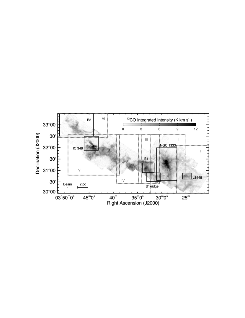
Figure 1.— ¹³CO(1-0) integrated intensity map of the Perseus molecular cloud complex from the COMPLETE survey (Ridge et al. 2006a). The six areas visualized in 3D Slicer are labeled I through VI. The black (solid line) boxes show the approximate boundaries of the star-forming regions used in our analysis in section 5 (see also Tables 4 and 5). Note that the ¹³CO map is not corrected for the FCRAO beam efficiency.

Large-scale (unbiased) molecular outflow surveys in the 1980’s were crucial in estimating the molecular outflow energy in whole clouds, and acknowledging that outflows can have a significant impact on their host cloud. These surveys were conducted toward clouds with high-mass star formation —i.e., Mon OB1 (Margulis & Lada, 1986) and the Orion southern cloud (Fukui et al., 1986)— using small (4 to 5 m) millimeter telescopes resulting in large beams (2.3′ to 2.7′). Only regions with detectable high-velocity gas ($v>10$ km s^-1) were then mapped at higher (sub-arcminute) resolution. Beam dilution should have hampered the ability to detect small ( $<0.4$ pc) and slow ($v<10$ km s^-1) outflows in these surveys and many such outflows were probably missed. Comparing recent higher angular resolution observations of small regions included within the large-scale surveys conducted about two decades ago, it is clear that these surveys detected only the most powerful outflows and that individual outflows were not resolved in high-density regions; compare, for example, the results of Yu et al. (2000) and Fukui et al. (1986).

Most of the recent outflow studies are restricted to small fields, focusing on individual objects or small dense regions of known star formation activity, thereby providing a limited view of the outflows’ impact on the environment at large (cloud) scales. These biases inhibit a full census of the outflows in a cloud, prevent the identification of multi-parsec outflows, and limit the study of the outflows’ impact on the entire molecular cloud complex. For example, the studies of Hatchell et al. (2007) and Hatchell & Dunham (2009) present a search for outflows towards known cores in the Perseus molecular cloud complex, and the study succeeds in deriving outflow properties of outflows in the Perseus cloud in a consistent way and finding a few new (previously undetected) outflows. However, they fail to provide an unbiased survey of outflows across the entire Perseus cloud complex as most observations are concentrated within $\sim 0.15$ pc from known cores and regions of active star formation. In contrast, the outflow survey presented here covers the full extent of the Perseus molecular cloud complex, and has the advantage of being able to provide information on how individual and groups of outflows effect the dynamics of the gas in the entire cloud complex and how they interact with their surroundings at different distances from the driving source (from about 0.06 pc to a few parsecs).

The Perseus molecular cloud complex is a chain of clouds with a total mass of a few thousand solar masses, and encompasses a total area of about 70 pc² (Evans et al., 2009). There is a span of distance estimates to Perseus that range from 230 pc (Cernis, 1990) to 350 pc (Herbig & Jones, 1983), most probably because different regions of the cloud complex are at different distances along the line of sight, and thus using a single distance for the entire cloud may be inappropriate. However, accurate distance estimates require maser parallaxes with high accuracy (e.g., Hirota et al. 2008), which do not yet exist for the entire cloud. To simplify our calculations, we adopt a single fiducial distance of 250$\pm$50 pc, similar to other recent cloud-wide studies of Persues (Enoch et al., 2006; Jørgensen et al., 2006; Ridge et al., 2006a; Rebull et al., 2007; Evans et al., 2009), and caution that there may be significant differences in the distance to different parts of the cloud. Perseus contains two rich protostellar clusters, IC 348 and NGC 1333, and a number of other regions of active star formation including B5, B1, L1448, and L1455 (see Figure 1). Surveys in the infrared, sub-millimeter, and millimeter reveal a large population of low-mass pre-main sequence stars, embedded protostars, and starless cores in Perseus (Ladd et al., 1993; Aspin et al., 1994; Lada & Lada, 1995; Hatchell et al., 2005; Enoch et al., 2006; Kirk et al., 2006; Muench et al., 2007; Gutermuth et al., 2008; Evans et al., 2009). Only one B5 star in IC 348 (HD 281159) is confirmed to reside in the Perseus cloud, but there might be a few other high-mass stars that interact with the cloud (through their winds and/or UV radiation) even though they were not necessarily formed in the cloud complex (see, e.g., Walawender et al. 2004; Ridge et al. 2006b; Kirk et al. 2006; Rebull et al. 2007). There is also a large number of nebulous objects associated with outflow shocks (i.e., HH objects and H₂ knots ) that have been identified in the cloud complex (Bally et al., 1996a, 1997; Yan et al., 1998; Walawender et al., 2005a; Davis et al., 2008).

The whole Perseus region was first surveyed in ¹²CO by Sargent (1979), and since then has been mapped in CO at different angular resolutions (all with beams $>1\arcmin$) by a number of other authors (e.g., Bachiller & Cernicharo, 1986; Ungerechts & Thaddeus, 1987; Padoan et al., 1999; Sun et al., 2006). These maps show a clear velocity gradient in the Perseus molecular cloud complex where the central cloud (LSR) velocity increases from about 4.5 km s^-1 at the western edge of the cloud to about 10 km s^-1 at the eastern end. The large velocity gradient in the gas across the entire complex and the fact that different parts of the Perseus cloud appear to have different distances (see above) could possibly indicate that the complex is made up of a superposition of different entities. Recently, the Perseus molecular cloud complex was also observed (and studied) in its entirety in the mid- and far-infrared as part of the “From Molecular Cores to Planet-forming Disks” (ak.a., c2d) Spitzer Legacy Project (Jørgensen et al., 2006; Rebull et al., 2007; Evans et al., 2009).

2. Data

In this paper, we use the ¹²CO(1-0) and ¹³CO(1-0) data collected for Perseus as part of the COMPLETE (COordinated Molecular Probe Line Extinction Thermal Emission) Survey of Star Forming Regions, described in detail by Ridge et al. (2006a). The ¹²CO and ¹³CO molecular line maps were observed between 2002 and 2005 using the 14-meter Five College Radio Astronomy Observatory (FCRAO) telescope with the SEQUOIA 32-element focal plane array. The receiver was used with a digital correlator providing a total bandwidth of 25 MHz over 1024 channels. The ¹²CO J=1-0 (115.271 GHz) and the ¹³CO J=1-0 (110.201 GHz) transitions were observed simultaneously using an on-the-fly (OTF) mapping technique. The beam telescope at these frequencies is about $46\arcsec$. Both maps of ¹²CO and ¹³CO are essential for a thorough study of the outflow and cloud properties. The ¹²CO(1-0) is a good tracer of the cool and massive molecular outflows and provides the information needed to study the impact of these energetic phenomena on the cloud. The ¹³CO(1-0) provides an estimate of the optical depth of the ¹²CO(1-0) line and can be used to probe the cloud structure and kinematics.

Observations were made in $10\arcmin\times 10\arcmin$ maps with an effective velocity resolution of 0.07 km s^-1. These small maps were then patched together to form the final large map of Perseus, which is about $6.25\arcdeg\times 3\arcdeg$. Calibration was done via the chopper-wheel technique (Kutner & Ulich 1981), yielding spectra with units of $T_{A}^{*}$. We removed noisy pixels that were more than 3 times the average rms noise of the data cube, the entire map was then resampled to a $46\arcsec$ grid, and the spectral axis was Hanning smoothed (necessary to keep the cubes to a size manageable by the 3D visualization code, see below). During the observations of the Perseus cloud, different OFF positions were used depending on the location that was being mapped. Some of these OFF positions had faint, though significant, emission which resulted in an artificial absorption feature in the final spectra. Gaussians were fitted to the negative feature in regions with no gas emission, and the fits were then used to correct for the contaminating spectral component. The resulting mean $3-\sigma$ rms per channel in the ¹²CO and ¹³CO maps are 0.25 and 0.20 K, respectively, in the $T_{A}^{*}$ scale. Spectra were corrected for the main beam efficiencies of the telescope (0.49 and 0.45 at 110 and 115 GHz, respectively), obtained from measurements of Jupiter.

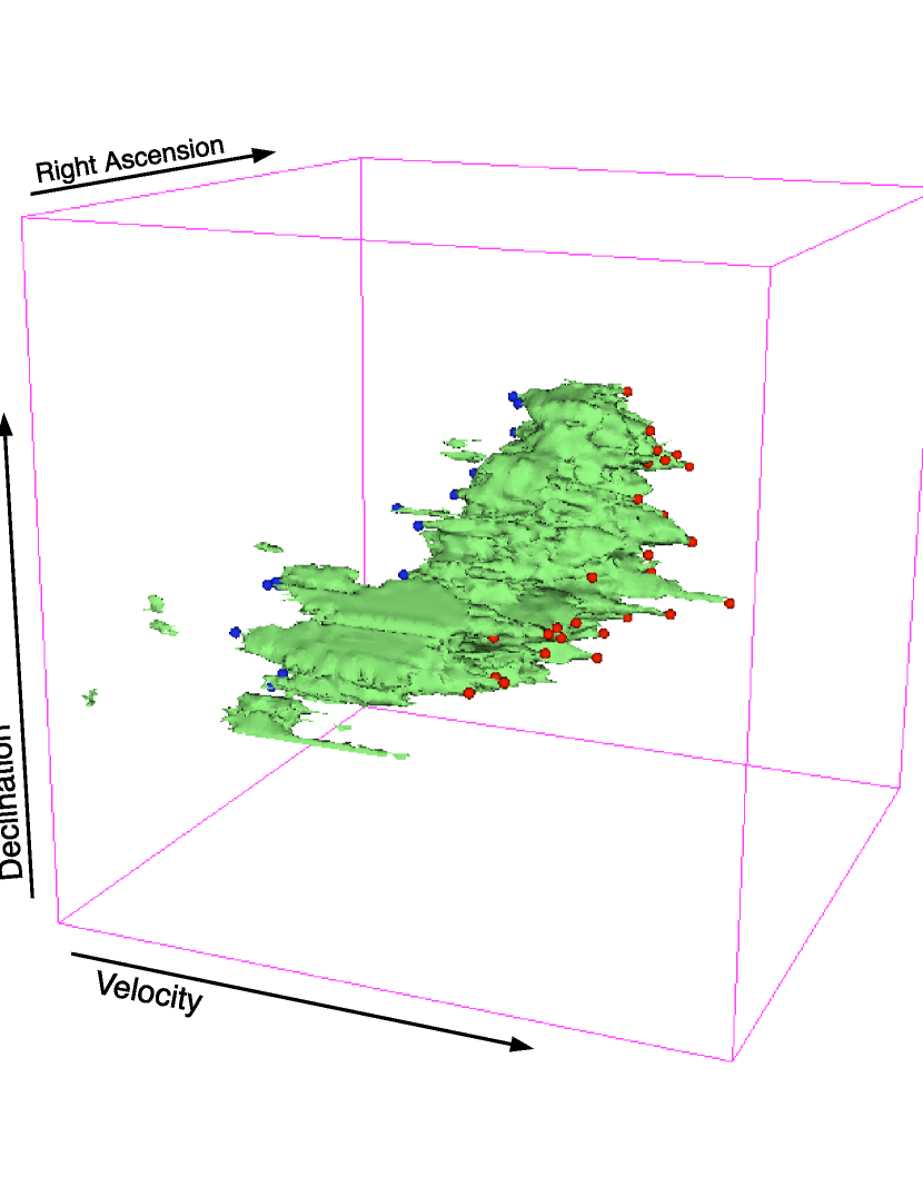
Figure 2.— Three-dimensional rendering of the molecular gas in B5 (i.e., Area VI in Figure 1), using 3D Slicer. The green isosurface model shows the ¹²CO emission in position-position-velocity space. The small circles show the locations of identified high-velocity points.

3. Computational Motivation and 3D Visualization

This study allows for a test of the effectiveness of 3D visualization of molecular line data of molecular clouds in RA-DEC-Velocity (p-p-v) space as a way to identify velocity features, such as outflows, in large maps. The primary program used for 3D visualization is 3D Slicer which was developed originally at the MIT Artificial Intelligence Laboratory and the Surgical Planning Lab at Brigham and Women s Hospital. It was designed to help surgeons in image-guided surgery, to assist in pre-surgical preparation, to be used as a diagnostic tool, and to help in the field of brain research and visualization (Gering, 1999). 3D Slicer was first used with astronomical data by Borkin et al. (2005) to study the hierarchical structure of star forming cores and velocity structure of IC 348 with ¹³CO(1-0) and C¹⁸O(1-0) data.

We divided the Perseus cloud into six areas (with similar cloud central LSR velocities) for easier visualization and outflow search in 3D Slicer (see below). The borders of these areas are similar to those named by Pineda et al. (2008), who also based their division mainly on the cloud’s central LSR velocity. The regions, whose outlines are shown in Figure 1, overlap between 1-3 arcminutes to guarantee complete analysis. This overlap was checked to be sufficient based on the fact that new and known outflows which crossed regions were successfully double-identified.

For each area, an isosurface (constant intensity level) model was generated in 3D Slicer, using the ¹²CO(1-0) map. The threshold emission intensity level chosen for each isosurface model was the lowest level of emission above the rms noise level for that particular region. This creates a 3D model representing all of the detected emission. The high velocity gas in this 3D space can be identified in the form of spikes, as shown for the B5 region in Figure 2, which visually stick out from the general distribution of the gas. These sharp protrusions occur since one is looking at the radial velocity component of the gas along the line of sight, thus causing spikes wherever there is gas at distinct velocities far away from the main cloud velocity. Instead of having to go through each region and carefully examine each channel map, or randomly scroll through the spectra by hand, this visualization allows one to instantly see where the high velocity points are located (see also Borkin et al., 2007, 2008).

Figure 3.— Spitzer IRAC color image of the c2d coverage of the Perseus cloud (Evans et al. 2009). The color code is blue (3.6µm), green (4.5µm), and red (8.0 µm). Ellipses and squares with rounded corners show the approximate regions where previously known outflows in Perseus lie. The grey contours show the 4 K km s^-1 level of the ¹³CO(1-0) integrated intensity map (not corrected for the FCRAO beam efficiency).

4. Outflow Identification

A total of 218 high velocity points were visually identified in 3D Slicer for all of Perseus in ¹²CO. We checked the position of each high-velocity point against the locations of known outflows (based on an extensive literature search) to determine if the point is associated with any known molecular outflow. From the 218 high-velocity points found, a total of 36 points were identified as associated with known molecular outflows. Figure 3 show the approximate regions where previously known ¹²CO(1-0) outflows lie. The number of high velocity points associated with a single outflow varies depending on its size and intensity. For example, the parsec-scale B5 IRS1 outflow is a conglomerate of 6 high velocity points whereas the HH 211 outflow, which is only $\sim 0.1$ pc long, is identified by only one point. We inspected each of the remaining 182 high-velocity points to verify whether they are outflow-related or caused by other velocity features in the cloud. To determine if a high-velocity point is outflow-related, we checked the spectrum by eye to look for outflow traits (e.g., high velocity low-intensity wings) and verified its proximity to known outflows and outflow sources (Wu et al., 2004), HH objects (Walawender et al., 2005a), H₂ knots (Davis et al., 2008), candidate young stellar objects (YSOs) form the c2d Spitzer survey (Evans et al., 2009) and other known outflow sources and YSOs. We also checked the velocity distribution and morphology of the gas associated with each high-velocity point to verify whether the velocity and structure of the gas were significantly different from that of the cloud in that region. From the remaining 182 high-velocity points found, a total of 60 points were classified as being outflow candidates based on the criteria mentioned above. For 97% of these outflow candidates, the maximum velocity away from the cloud velocity is equal to or greater than the escape velocity in that region of the cloud. We note that we purposely chose not to be too restrictive in the definition of outflow candidate (e.g., we identified outflow candidates even without a solid outflow source identification, see below). Using our broad, yet realistic, definition we can calculate the maximum possible impact from all plausible molecular outflows to the cloud. Out of the remaining 122 points, 17 points were discarded due to too much noise or being pixels cut-off by the map’s edge and the other 105 points are thought to be caused by a number of other kinematic phenomena, including clouds at other velocities in the same line of sight unrelated to the Perseus cloud and spherical winds from young stars that produce expanding shell-like structures in the molecular gas (as opposed to the discrete blob morphology observed in the 60 outflow candidates). The distribution and impact of these expanding shells on the cloud will be discussed further in a subsequent paper (Arce et al., in preparation)

Table 1Candidate New and Extended Outflow Locations

Name	RA	DEC	Area	Mass	Momentum	Kinetic Energy	Driving Source
	(J2000)		(arcmin)	(M☉)	(M☉ km s-1)	(1042 ergs)	Candidate(s)
CPOC 1	03:23:21	30:52:10	$19\times 12$	0.05	0.19	6.93	L1448-IRS1
CPOC 2	03:23:54	30:48:10	$16\times 7$	0.36	0.88	21.68	L1448-IRS1
CPOC 3	03:24:30	30:50:00	$10\times 5$	0.02	0.08	2.93	L1448-IRS3
CPOC 4	03:24:54	30:43:10	$4\times 4$	0.01	0.04	2.10	multiple in L1448
CPOC 5	03:25:39	30:28:20	$7\times 5$	0.02	0.05	1.32	SSTc2dJ032519.52+303424.2
CPOC 6	03:27:55	31:19:50	$4\times 3$	0.02	0.03	0.36	multiple NGC1333, near HH338
CPOC 7	03:28:00	31:03:40	$15\times 12$	0.29	1.79	112.00	SSTc2dJ032834.49+310051.1
CPOC 8	03:28:32	30:28:20	$8\times 11$	0.11	0.28	7.17	near HH750 and HH743, SSTc2dJ032835.03+302009.9 or SSTc2dJ032906.05+303039.2
CPOC 9	03:28:28	31:13:20	$8\times 8$	0.26	0.56	12.63	SSTc2dJ032832.56+311105.1 or SSTc2dJ032837.09+311330.8
CPOC 10	03:28:27	31:23:20	$8\times 8$	0.24	0.42	7.50	SSTc2dJ032844.09+312052.7
CPOC 11	03:28:40	31:07:10	$8\times 6$	0.11	0.27	7.01	STTc2dJ032834.53+310705.5
CPOC 12	03:28:43	31:07:30	$8\times 7$	0.19	0.97	52.02	SSTc2dJ032843.24+311042.7
CPOC 13	03:28:50	31:27:10	$6\times 8$	0.31	0.80	21.00	multiple in NGC1333
CPOC 14	03:28:57	30:50:20	$6\times 5$	0.03	0.05	0.73	SSTc2dJ032850.62+304244.7 or SSTc2dJ032852.17+304505.5
CPOC 15	03:29:07	30:45:50	$7\times 5$	0.19	0.80	32.82	SSTc2dJ032850.62+304244.7 or SSTc2dJ032852.17+304505.5
CPOC 16	03:29:30	31:07:10	$6\times 6$	0.04	0.10	2.40	HH18A, multiple in NGC1333
CPOC 17	03:29:41	31:17:30	$9\times 13$	3.20	8.49	235.28	near HH497, HH336, multiple in NGC1333
CPOC 18	03:29:41	31:27:10	$5\times 6$	0.08	0.21	6.35	HH764, multiple in NGC1333
CPOC 19	03:29:27	31:34:00	$9\times 7$	0.19	0.59	19.31	IRAS03262+3123
CPOC 20	03:30:06	31:27:10	$5\times 4$	0.04	0.08	1.73	multiple NGC1333
CPOC 21	03:30:11	31:14:00	$8\times 5$	0.05	0.13	3.45	HH767, SSTc2dJ033024.08+311404.4
CPOC 22	03:30:40	30:37:00	$6\times 11$	0.30	1.07	39.24	multiple in Per6 aggregate
CPOC 23	03:30:56	31:21:10	$6\times 6$	0.01	0.05	3.56	multiple in NGC1333 or B1
CPOC 24	03:31:23	31:01:30	$27\times 18$	0.46	2.99	193.71	multiple in B1 or B1-Ridge
CPOC 25	03:31:23	31:20:40	$4\times 7$	0.02	0.14	9.73	multiple in NGC1333 or B1
CPOC 26	03:31:40	30:54:40	$6\times 4$	0.09	0.27	8.26	IRAS03292+3039 or others in B1 and B1-Ridge
CPOC 27	03:31:54	31:14:10	$8\times 5$	0.07	0.40	21.85	multiple in NGC133 or B1
CPOC 28	03:32:04	30:40:20	$4\times 5$	0.58	1.35	31.94	multiple in B1-Ridge
CPOC 29	03:32:25	31:18:10	$5\times 7$	0.06	0.17	4.89	multiple in B1
CPOC 30	03:32:37	31:02:50	$3\times 6$	0.04	0.13	3.57	multiple in B1
CPOC 31	03:32:58	31:22:20	$4\times 8$	0.15	0.37	9.32	SSTc2dJ033312.84+312124.2 or SSTc2dJ033313.80+312005.3
CPOC 32	03:33:14	30:59:00	$4\times 6$	0.07	0.17	4.25	SSTc2dJ033346.92+305350.1 or multiple in B1 core
CPOC 33	03:33:40	31:28:50	$5\times 6$	0.21	0.50	11.77	multiple in B1
CPOC 34	03:33:58	31:16:10	$6\times 4$	0.14	0.25	4.58	SSTc2dJ033401.66+311439.8
CPOC 35	03:34:43	31:22:00	$5\times 8$	0.10	0.24	5.43	SSTc2dJ033430.78+311324.4 or SSTc2dJ033449.84+311550.3
CPOC 36	03:35:10	31:18:00	$4\times 5$	0.11	0.30	8.02	SSTc2dJ033430.78+311324.4 or SSTc2dJ033449.84+311550.3
CPOC 37	03:38:58	32:05:50	$5\times 3$	0.16	0.19	2.34	unknown between IC348 and B1
CPOC 38	03:39:05	32:08:40	$5\times 4$	0.04	0.06	0.90	unknown between IC348 and B1
CPOC 39	03:39:11	31:19:00	$8\times 8$	0.10	0.19	3.83	SSTc2dJ033915.81+312430.7 or SSTc2dJ034001.49+311017.3
CPOC 40	03:39:16	32:18:10	$6\times 4$	0.09	0.24	11.17	IRAS03363+3207
CPOC 41	03:39:18	31:58:10	$7\times 6$	0.14	0.21	3.22	IRAS03367+3147
CPOC 42	03:39:20	32:17:40	$5\times 5$	0.20	0.19	1.92	IRAS03363+3207
CPOC 43	03:40:24	32:04:00	$7\times 8$	2.04	3.89	76.37	IRAS03367+3147 or multiple west of IC348
CPOC 44	03:42:12	31:51:50	$5\times 5$	0.09	0.18	3.44	multiple east of IC348
CPOC 45	03:44:34	31:58:20	$4\times 6$	0.54	0.73	10.04	multiple in south edge of IC348
CPOC 46	03:44:53	32:14:40	$11\times 6$	0.33	0.66	13.19	multiple in north edge of IC348
CPOC 47	03:44:58	32:32:00	$11\times 9$	0.20	0.41	8.69	multiple in north edge of IC348
CPOC 48	03:45:01	31:57:50	$4\times 4$	0.16	0.25	3.94	multiple in south edge of IC348
CPOC 49	03:45:04	32:00:30	$5\times 5$	0.03	0.09	3.40	multiple in south edge of IC348
CPOC 50	03:45:26	31:58:00	$6\times 6$	0.25	0.36	5.29	multiple in south edge of IC348
CPOC 51	03:45:53	32:34:00	$7\times 7$	0.27	0.32	4.09	B5-IRS1
CPOC 52	03:45:59	32:42:50	$7\times 7$	0.13	0.29	6.55	unknown in B5
CPOC 53	03:46:54	32:36:20	$6\times 5$	0.07	0.10	1.24	B5-IRS3
CPOC 54	03:47:16	32:39:50	$5\times 4$	0.06	0.09	1.48	B5-IRS3
CPOC 55	03:47:17	33:01:40	$15\times 15$	3.97	7.55	147.19	B5-IRS4?
CPOC 56	03:47:60	32:38:40	$20\times 13$	3.76	6.73	124.04	multiple in B5
CPOC 57	03:48:01	33:14:40	$6\times 6$	0.09	0.11	1.45	B5-IRS4?
CPOC 58	03:49:14	32:57:40	$7\times 6$	0.28	0.27	2.83	unknown in B5
CPOC 59	03:49:18	33:04:40	$5\times 7$	0.20	0.25	3.37	B5-IRS1
CPOC 60	03:49:41	33:12:20	$8\times 7$	0.58	0.64	7.08	unknown in B5

We visually inspected the velocity maps in the area surrounding each of the 60 high-velocity points identified as outflow in origin (but unrelated to known outflows) and chose an area (in RA-Dec space) and velocity range that included all or most of the emission associated with the kinetic feature. The integration area and velocity ranges were conservatively chosen to include only the emission visibly associated with the outflowing material, thus avoiding cloud emission. The high-velocity gas associated with these 60 points show discrete morphologies in area and velocity. Hereafter each of these high-velocity features is referred as a “COMPLETE Perseus Outflow Candidate” (CPOC) and we list their positions and other properties in Table 1. In Figure 4 we show the velocity ranges of all CPOCs, in comparison with their local cloud (LSR) velocity.

Our outflow-detection technique proved to be reliable, as we detect high-velocity gas associated with all published CO(1-0) outflows (see Figure 3). However, it is very probable that the catalog of new molecular outflows generated for this paper is an underestimate of the true number of previously undetected molecular outflows due to the resolution of the CO maps and other limitations of our outflow-detection technique. Unknown outflows that are smaller than the beam size of our map (i.e., $0.06$ pc at the assumed distance of Perseus) or that have weak high-velocity wings (i.e., with intensities less than twice the rms of the spectra at that particular position) cannot not be detected by our technique. Outflows with maximum velocities too close to the ambient gas velocity to produce a detectable high-velocity spike in $p-p-v$ space are also missed by our procedure, as well as high-velocity gas in regions “contaminated” by unrelated clouds along the same line-of-sight. Although we are able to detect high-velocity outflow gas in regions with a high density of protostars, our map’s beam size limits our ability to distinguish individual outflows in dense clusters like NGC 1333. Higher resolution maps would be needed to identify the individual molecular outflows in regions with a high-density of protostars. However, the technique used in this paper proved ideal for finding parsec-scale outflows and identifying outflows over large areas.

Although most molecular outflows in Perseus are in well-known regions of active star formation (i.e, L1448, NGC 1333, B1, IC 348, and B5) we also detected high-velocity features associated with molecular outflows across the whole expanse of the cloud complex. The locations of all the CPOCs can be seen in Figures 5 to 10. From these figures it is clear that most of the new outflow candidates are located around the edges of clusters (e.g., CPOCs 16 to 22 around NGC 1333, and CPOCs 48 to 50 in the outskirts of the IC 348 cluster), or were identified in cloud regions between clusters (e.g., CPOCs 38 to 42). By surveying the entire cloud complex and regions between clusters, we were able to identify previously-undetected outflows and extensions of known outflows in the poorly-studied regions of the Perseus cloud complex. We discuss all candidate outflows and their possible association with nearby protostellar sources, HH objects and H₂ knots in the Appendix.

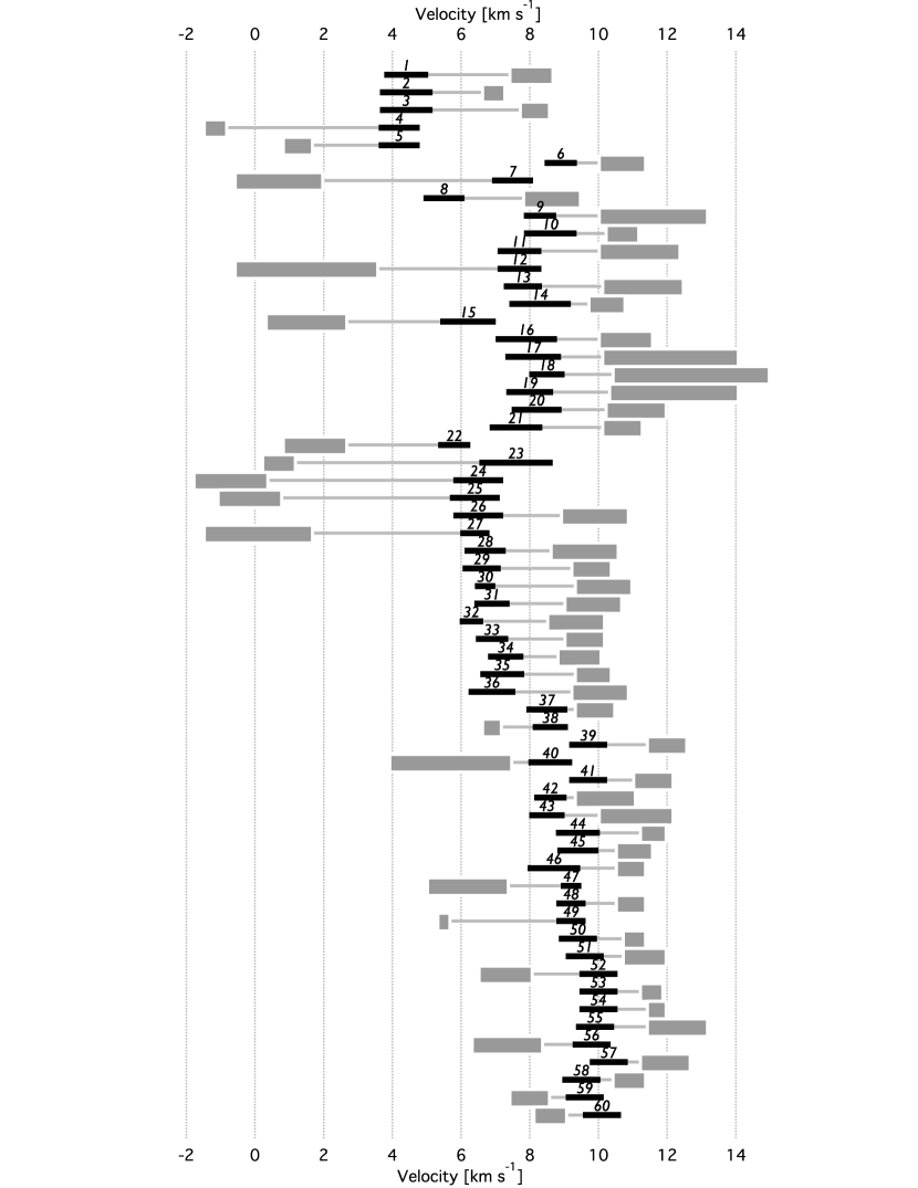
Figure 4.— Velocity of CPOCs with respect to the local cloud central (LSR) velocity. Black (thick) horizontal lines are centered on the CPOC area’s central LSR velocity and their extent represent the velocity dispersion of the cloud, as measured from the average ¹³CO spectra over the CPOC area (see Table 1). The grey horizontal rectangles indicate the range of velocities for each CPOC. Numbers above each black line refer to the CPOC number.

4.1. Outflow Source and Counter-Lobe Identification

For many of the new outflow candidates it is hard to unambiguously assign a source. Pervious studies show that not all molecular outflows have lobes that originate close to the source and extend with a continuous structure all the way to the outflow’s terminus. Instead, many molecular outflows are composed of discrete high-velocity blobs along their axes produced by different mass ejection episodes (e.g., Cernicharo & Reipurth 1996; Yu et al. 1999; Arce & Goodman 2001a; Arce & Goodman 2002b). In some cases the high-velocity CO blobs coincide with one or more HH objects, while in other cases there are no shock tracers in the vicinity of the outlowing gas. In addition, a number of known processes including precession (Terquem et al., 1999), a relative motion between the outflow source and the ambient medium (Bally & Reipurth 2001; Masciadri & Raga 2001; Goodman & Arce 2004), and collision with a denser environment (Raga et al., 2002) may cause the axis of an outflow to change over time. The episodic nature of outflows as well as possible variations in their axes make the reliable identification of an outflowing blob’s source difficult, especially in regions with a dense population of young stellar objects. It is, therefore, no surprise that our data does not allow us to determine for certain the sources associated with the listed CPOCs. Nonetheless, in Table 1 we give possible candidate sources based on their proximity to the CPOCs. In addition to the factors listed above, the fact that sometimes molecular outflows have one detectable lobe —either due to contamination from another cloud along the same line of sight or the fact that the other lobe breaks out from the molecular cloud— makes it very difficult to pair each CPOC with a corresponding counter lobe. Higher angular resolution CO maps in combination with spectroscopic and proper motion studies (to determine the three-dimensional velocity) of nearby HH objects should allow the proper identification of the source and coounter-lobe for most CPOCs.

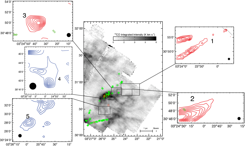
Figure 5.— CPOCs in Area I. The grey-scale image shows the ¹³CO integrated intensity. Star symbols indicate the position of candidate YSOs from the c2d survey and known outflow and IRAS sources, while diamonds represent HH objects and H₂ outflow shock emission. Integrated intensity contour maps of the CPOCs in Area I are shown. Redshifted (blueshifted) CPOCs are shown in black (grey) contours. The velocity range of integration is that shown in Figure 4. For all panels the x-axis shows the Right Ascension (J2000), and the y-axis shows the Declination (J2000). The telescope beam is shown as a filled black circle in the lower part of each CPOC map. The ¹³CO map is not corrected for the FCRAO beam efficiency.

4.2. Outflow Candidates vs. Turbulence Features

Despite the fact that outflow-related high-velocity features could in principle be confused with turbulent-generated velocity structures, we are certain that most (if not all) CPOCs are outflow in origin. Numerical simulations show that line profiles from a medium with a random turbulent velocity field, such as a molecular cloud, will exhibit non-Gaussian features like double peaks, skewness, and high-velocity wings, even if generated using a Gaussian random field (Dubinski et al. 1995). This could lead to confusion between high-velocity turbulent-generated velocity features in the molecular line and high-velocity outflow-generated velocity features. However, observational studies show that at scales of a few tenths of parsecs (and densities of about $10^{4}$ cm^-3), most molecular clouds exhibit turbulence-related velocity features with maximum velocities of about 1 km s^-1 and all are less than 2 km s^-1 away from the central cloud velocity (Falgarone et al. 1998). Moreover, observations of clouds that are presumably free of star formation activity and where the only “high” velocity features should be caused by turbulence (or other clouds along the line of sight) the range in velocities of the emission is not more than 4 km s^-1 (see Falgarone et al. 1990; 1998; 2006; 2009). This implies that the highest velocity turbulence features are never more than 2 km s^-1 away from the line center. In contrast, most (i.e., 97%) of the candidate outflows listed in Table 1 have a maximum velocity that is greater than or equal to 2 km s^-1, and all have a maximum velocity that is 1.9 km s^-1 or more. In addition, all CPOCs have a maximum velocity that is 3.1 times (or more) than the cloud’s velocity dispersion ($\sigma_{cl}$) and 73% of the CPOCs have maximum velocities of more than 4.5 $\sigma_{cl}$ (see Figure 4). The velocities of turbulent generated features in terms of the velocity dispersion of the cloud are typically much lower than those exhibited by the CPOCs (see, e.g., Falgarone et al. 1990). The CPOCs’ high velocities, as well as their proximity to YSOs and HH objects makes it very likely that most (if not all) are outflow-related features, and not produced by pure random motions in the cloud’s turbulent gas.

5. Analysis & Discussion

5.1. Mass, Momentum and Energy of Outflows

We use a method to obtain the outflow mass similar to that described by Arce & Goodman (2001, hereafter AG01). This technique, which is based on the method employed by Bally et al. (1999) and Yu et al. (1999), uses the ¹²CO(1-0) to ¹³CO(1-0) ratio to estimate the opacity in the ¹²CO(1-0) line, as a function of velocity. In molecular clouds the ¹²CO(1-0) line is typically optically thick and its opacity depends on velocity. In the general, at high outflow velocities the opacity of the line is lower than the opacity of the line close to the cloud velocity. Using an optically thick line without properly correcting for its velocity-dependent opacity will result in an underestimation of the outflow mass, momentum, and kinetic energy.

We briefly describe the method here, but for more detail see AG01. For each candidate (or known) outflow we calculate average spectra of ¹²CO(1-0) and ¹³CO(1-0) over the defined outflow region (shown in Tables 1 and 2) in order to estimate the ratio of ¹²CO (1-0) to ¹³CO (1-0) as a function of velocity. The line ratios, hereafter denoted $R_{12/13}$, were each fitted with a second order polynomial as described in AG01. To calculate the outflow mass at a given position, we directly use the ¹³CO emission at low outflow velocities (given by the main beam corrected antenna temperature of the line, $T_{mb}^{13}$). At high outflow velocities, where the ¹³CO was not reliably detected, we use the ¹²CO (1-0) emission ($T_{mb}^{12}$) and the fit to $R_{12/13}(v)$ to estimate the value of $T_{mb}^{13}$ at the given velocity and position, using the simple equation $T_{mb}^{13}=T_{mb}^{12}/R_{12/13}(v)$. We then obtain a value of the ¹³CO opacity ($\tau_{13}$), from which we then obtain a value of the ¹³CO column density ($N_{13}$) and then the mass, using equations (1), (3), and (4) of AG01. We only use spectral data that is greater than or equal to three times the rms noise of the spectrum.

Table 2Properties of Known Outflows and Outflow Regions

Name	RA	DEC	Area	Velocity Range	Mass	Momentum	Kinetic Energy
	(J2000)		(arcmin)	(km s-1)	(M☉)	(M☉ km s-1)	(1042 ergs)
L1448 Outflows (blue)	03:24:32	30:50:10	$12\times 6$	[-5.0, -0.5]	0.06	0.34	21.0
L1448 Outflows (red)	03:25:25	30:40:30	$8\times 11$	[7.0, 16.0]	0.45	1.50	61.2
L1455 (blue)	03:26:40	30:18:50	$12\times 8$	[0.1, 2.5]	0.10	0.27	7.8
L1455 (red)	03:26:40	30:18:50	$12\times 8$	[7.6, 9.0]	0.11	0.34	11.0
IRAS 03262+3123 (red)	03:28:17	31:01:30	$4\times 3$	[9.5, 13.8]	0.08	0.29	10.7
NGC 1333 Outflows (red)	03:29:00	31:17:10	$12\times 14$	[10.2, 12.3]	1.35	4.22	142.5
	03:29:15	31:25:00	$5\times 8$	[10.2, 19.6]	0.49	1.18	28.7
NGC 1333 Outflows (blue)	03:29:03	31:16:20	$17\times 14$	[-0.6, 3.8]	0.50	2.62	142.0
	03:29:20	31:27:00	$12\times 8$	[-0.6, 0.8]	0.03	0.26	20.0
IRAS 03282+3035 (red)	03:31:09	30:47:00	$6\times 5$	[8.6, 11.8]	0.21	0.45	9.7
IRAS 03282+3035 (blue)	03:31:16	30:45:00	$9\times 6$	[-2.5, 1.2]	0.03	0.24	17.0
IRAS 03291+3039 (red)	03:32:18	30:47:30	$5\times 5$	[8.9, 11.2]	0.02	0.06	1.7
B1 Outflows (blue)	03:33:14	31:10:20	$12\times 12$	[-1.6, 1.0]	0.05	0.37	24.6
B1 Outflows (red)	03:33:14	31:10:20	$12\times 12$	[9.1, 12.5]	0.31	0.89	27.5
IC 348 Outflows (blue)	03:44:01	32:02:40	$8\times 13$	[5.8, 6.5]	0.79	1.89	45.4
IC 348 Outflows (red)	03:44:01	32:02:40	$8\times 13$	[10.3, 11.6]	2.05	3.73	68.8
B5-IRS1 (blue)	03:48:39	33:01:00	$9\times 6$	[6.5, 8.6]	0.77	1.36	25.2
	03:48:12	32:55:10	$8\times 4$	[5.8, 8.6]	0.93	1.79	36.3
	03:46:44	32:46:50	$8\times 7$	[7.1, 8.6]	0.35	0.67	13.1
B5-IRS1 (red)	03:48:26	32:57:30	$7\times 5$	[11.4, 12.8]	0.22	0.37	6.4
	03:47:17	32:50:40	$12\times 5$	[11.5, 14.4]	0.55	0.91	15.9
	03:46:46	32:44:30	$9\times 5$	[11.5, 14.4]	0.58	0.87	13.8

We estimate the excitation temperature, $T_{ex}$, for each CPOC assuming that the ¹²CO(1-0) line core is optically thick. We measured the peak temperature of each spectrum in the CPOC region, and use Equation 2 in AG01 to obtain a distribution of the ambient cloud $T_{ex}$ values within that area. We obtain an average $T_{ex}$ for each CPOC region, and assume that this average value is the temperature of the outflowing gas (at all velocities) in the entire CPOC region. Pineda et al. (2008) found slight variations (from 2.8 to 4.9 $\times 10^{5}$) in the ratio of molecular hydrogen to ¹³CO depending on the region in Perseus. We used their region-dependent values of [H₂]/[¹³CO] and the ratio of ¹²CO to ¹³CO of 62 (from Langer & Penzias 1993). We obtain the line-of-sight outflow momentum, $P_{out}$, using

$$P_{out}=\sum_{v}M(v_{out})v_{out}$$ (1)

where $v_{out}$ is the line-of-sight component of the outflow velocity and $M(v_{out})$ is the outflow mass as a function of (line-of-sight) outflow velocity. The outflow velocity is defined as $v_{out}=v_{obs}-v_{amb}$, where $v_{obs}$ and $v_{amb}$ are observed and ambient cloud LSR velocities, respectively. For each CPOC we obtain a value of $v_{amb}$ (i.e., the line core velocity) by fitting a Gaussian to the average ¹³CO(1-0) spectrum over the CPOC area. The outflow kinetic energy, $E_{out}$, using only the line-of-sight component of the velocity is obtained with:

$$E_{out}=0.5\sum_{v}M(v_{out})v_{out}^{2}$$ (2)

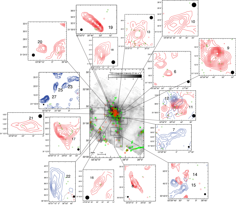
Figure 6.— CPOCs in Area II. The rest is the same as in Figure 5

The numbers shown in Tables 1 and 2 represent lower limits, as there are several outflow properties that have not been taken into consideration when estimating the outflow mass, momentum, and energy which increase the total estimates. As discussed in Section 4, we conservatively define the lowest outflow velocity as the velocity for which we are certain that most (or all) of the emission within the defined area arises from the outflow (i.e., there is little or no cloud emission in the region). This results in an under-estimation of the outflow mass (as well as energy and momentum), as we are not including the outflow emission “hidden” under the cloud line emission. Previous outflow studies indicate that failing to account for this hidden component will underestimate the mass by at least a factor of two (as shown by, e.g., Margulis & Lada 1985).

The assumed value of the outflow temperature can also affect the outflow mass estimates. We use the average excitation temperature of the cloud in the outflow region to estimate the outflow mass, as it is the only estimate of the gas temperature we can obtain with our data. Outflow studies that observe different transitions of the same molecule show that temperatures of outflowing molecular gas are higher than the cloud’s excitation temperature and is not uncommon for outflows to reach temperatures of 50 to 100 K (e.g., Hirano & Taniguchi 2001; van Kempen et al. 2009). When using the ¹²CO(1-0) emission to derive outflow properties, the dependence of CO column density with excitation temperature is such that an increase in the temperature above 10 K will result in an increase in the estimate of the outflow mass (see Appendix in Lada & Fich 1996). If we assume that typical outflow temperatures are about 3 times higher than the cloud excitation temperature, the resulting estimate of the outflow mass, momentum, and energy would increase by a factor of about 2.5. Combing this factor and a factor of two to correct for the unaccounted outflow emission hidden under the cloud emission, we reckon that our original estimates of the outflow mass should increase by a factor of 5.

The values of the outflow momentum and energy shown in Tables 1 and 2 only take into consideration the line-of-sight outflow velocity component. If we assume an average outflow inclination of $45\arcdeg$, the momentum and energy estimates increase by factors of 1.4 and 2, respectively. Also, some of the shocks that produce these outflows may be dissociative (see Reipurth & Bally 2001), and thus in some outflows a fraction of the outflow momentum and energy may not be traceable by the CO emission. Combining these factors with the correction factor for the outflow mass, we estimate that to obtain reasonable values of the outflows’ momentum, and kinetic energy our original estimates should increase by “correction” factors of 7 and 10, respectively.

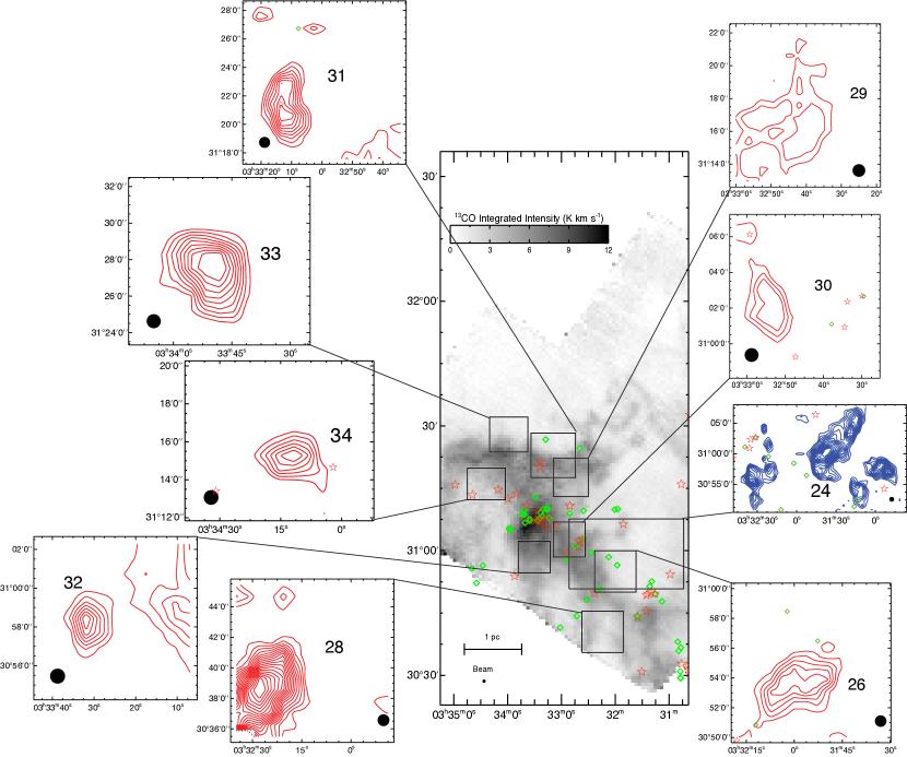
Figure 7.— CPOCs in Area III. The rest is the same as in Figure 5.

The total mass, momentum and energy of all outflows in our maps (i.e., CPOCs and previously known outflows) are 163 M_☉, 517 M_☉ km s^-1, and $20.5\times 10^{45}$ erg, respectively (using the correction factors discussed above). If we only include the numbers for the previously known outflows, the totals are 51 M_☉, 173 M_☉ km s^-1, and $7.5\times 10^{45}$ erg (see Table 3). Our study shows that in Perseus there is much more outflowing mass and considerably more injection of momentum and energy by outflows into the cloud than previously thought, as the new CPOCs more than double the total outflow mass, momentum, and kinetic energy in the Perseus molecular cloud complex. It is clear that large-scale observations like the ones used in this study are necessary to obtain a complete picture of the impact of outflows on their entire host cloud.

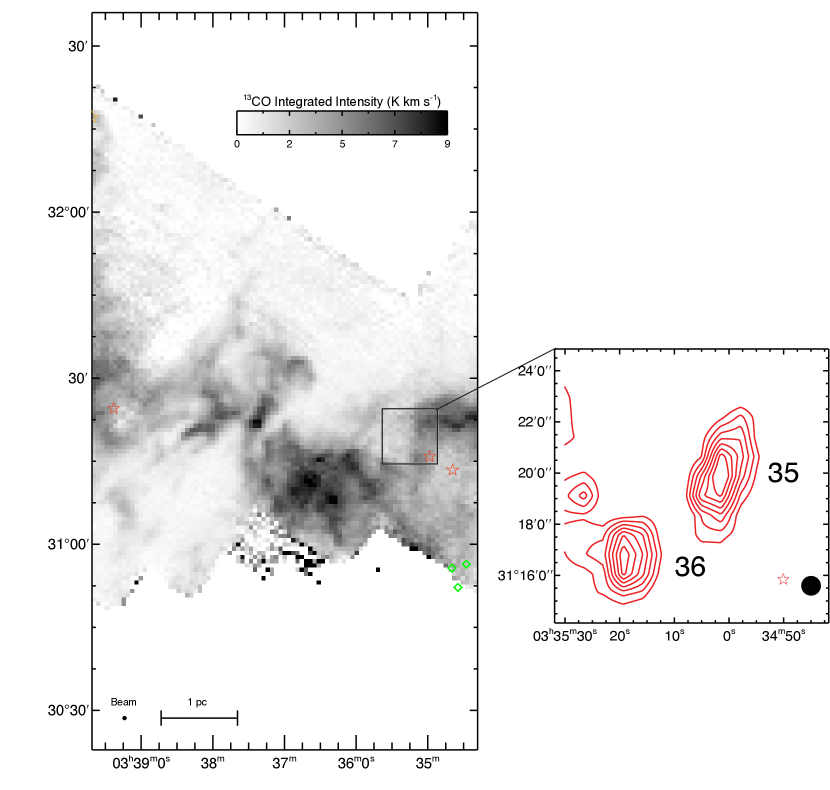
Figure 8.— CPOCs in Area IV. The rest is the same as in Figure 5.

5.2. The Impact of Outflows in Perseus

With our cloud-wide survey we can assess the impact of outflows on the Perseus complex as a whole by comparing the total energy and momentum of all the observed outflows with the cloud complex’s energetics. From the COMPLETE molecular line data (and using the procedure described above), we obtain a mass for the observed Perseus cloud complex of approximately $7\times 10^{3}$ M_☉. The average velocity width (FWHM) is about 2 km s^-1, so the turbulent energy of the complex is $E_{turb}\sim 1.6\times 10^{47}$ erg. The total kinetic energy from all the observed outflows (using the correction factor discussed above) is $2\times 10^{46}$ ergs, only 13% of the turbulent energy of the entire complex. Even with the considerable increase in the outflow energy and momentum injection with the new outflow candidates reported here, it is evident that the energy input solely by protostellar outflows is not enough to feed the observed turbulence in the cloud. This should not come as a surprise, as although we find numerous outflows in the cloud they are mostly found in concentrated regions of star formation and there are large extents of molecular gas in the complex with few or no outflows. This implies that an additional energy source is responsible for turbulence on a global cloud scale in the Perseus complex. In a subsequent paper we propose that expanding shells produced by spherical winds (and soft-UV radiation) from stars in, and near, the cloud can provide the additional energy required to drive and maintain the turbulence throughout the entire cloud complex (Arce et al., in preparation).

The clustering of outflows in localized star forming regions indicates the possibility that although the outflows might only have a small impact on the Perseus complex as a whole, they still may have considerable impact on their immediate environment. We define six regions of active star formation in the Perseus molecular cloud complex where we find a cluster or group of outflows: L1448, NGC 1333, B1-ridge, B1, IC 348, and B5. The locations of these regions within the cloud complex and their extent are shown in Figure 1 and Table 4, their physical properties are shown in Table 5, and the total outflow mass, momentum and energy within these regions are shown in Table 6. In order to quantitatively assess the impact of outflows on their local environment, we compare the outflow energy and momentum with their host region’s energetics.

5.2.1 Outflows and Turbulence

A comparison between the total outflow kinetic energy in each region and the region’s turbulent energy shows that the total energy of outflows is between about 14 and 80% of the total turbulent energy of the region (see Table 7). This suggests that in some regions, outflows in a localized area of star formation inside a cloud complex can inject a significant amount of energy into the gas to considerably affect the turbulence of the local environment.

Table 3Perseus Outflow Properties

Objects	Mass	Momentum	Kinetic Energy
	(M☉)	(M☉ km s-1)	(1044 ergs)
Known Outflows	10.1 / 51	24.7 / 173	7.5 / 75
CPOCs	22.3 / 112	49.2 / 344	13.0 / 130
Total	32.4 / 163	73.9 / 517	20.5 / 205

Another way to assess the importance of outflows in driving the turbulence in their local environment is to compare the total outflow energy input rate into the cloud (i.e., outflow luminosity) with the energy rate needed to maintain the turbulence in the gas. We estimate the outflow luminosity by dividing the outflow kinetic energy by an estimate of the outflow’s timescale, $\tau_{flow}$. This term introduces the biggest uncertainty in our estimate of the outflow luminosity as it is hard to determine the age of a molecular outflow solely from molecular line emission data (identification of the outflow source and measurement of the kinematics of the shocks associated with the outflow are needed to obtain a relatively accurate outflow age). Most possible candidate sources listed in Table 1 are protostars in the Class I stage, as reported by Evans et al. (2009). This stage has an average lifetime of about 0.5 Myr (Evans et al., 2009), and consequently this provides an upper limit to the typical outflow ages in Perseus. A lower limit on the age of molecular outflows in Perseus is given by the time that a “typical” protostellar jet in Perseus has taken to reach its current position. We estimate this lower limit by assuming a typical jet velocity of 100 km s^-1 (Reipurth & Bally 2001) and a median jet lobe in Perseus (from infrared Spitzer images) of about 0.3 pc (Guenthner 2009), which results in a value of $3\times 10^{3}$ yr. Here we use a value between these two limits, $\tau_{flow}=5\times 10^{4}$ yr, for our estimation of the outflow luminosity and caution that there are major uncertainties in this assumption.

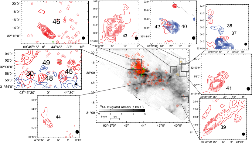
Figure 9.— CPOCs in Area V. The rest is the same as in Figure 5.

The numerical study by Mac Low (1999) shows that the energy dissipation of uniformly driven magnetohydrodynamic turbulence is approximately given by:

$$t_{diss}\sim(\frac{3.9\kappa}{M_{rms}})t_{ff}$$ (3)

where $M_{rms}$ is the Mach number of the turbulence (i.e., the ratio of the turbulence velocity dispersion over the sound speed), $t_{ff}=\sqrt{3\pi/32G\rho}$ is the free-fall timescale, and $\kappa=\lambda_{d}/\lambda_{J}$, the ratio of the driving wavelength over the Jean’s length of the clump. Numerical simulations show that the turbulence driving length of a continuous (i.e., non-episodic) outflow is approximately equal to the outflow lobe or cavity length (Nakamura & Li 2007; Cunningham et al. 2009). In a cluster, different outflows will inject their energy on a range of scales (Carroll et al. 2009), and depending on the length and number of episodic events, the driving scale could vary significantly between outflows. A study of infrared outflows in Perseus using IRAC Spitzer images shows that outflow lobes in this cloud can range from 0.03 to about 2 pc (Guenthner 2009). It is, therefore, difficult to assign a single value to $\lambda_{d}$. To simplify our analysis we choose $\kappa\sim 1$ to obtain an estimate of $t_{diss}$ using the equation above, and warn that for most outflows in our sample this is probably a lower limit as most molecular outflows detected in our maps are at least four beam sizes ($\sim 0.22$ pc) in length and the average $\lambda_{J}$ of the clumps is $\sim 0.2$ pc.

We estimate the average density of the region using $M_{reg}/R_{reg}^{3}$, and we assume the temperature of the gas is given by the average cloud excitation temperature in the region (see Table 5). The turbulent dissipation rate (i.e., the power needed to maintain the turbulence in the volume) is then given by $L_{turb}=E_{turb}/t_{diss}$ and it is shown for each region in Table 5. It can be seen that for all six regions the total outflow luminosity is at least 80% of $L_{turb}$ and that for five of the regions the outflow luminosity is significantly more ($\geq 150\%$) than the power needed to maintain the turbulence (see Table 7), implying that outflows are an important agent for the maintenance of turbulence in most regions of active star formation.

We note that the numerical study from which we obtained equation 3 uses parameters that are appropriate to conditions found in molecular clouds, yet the space dependence of the driving function in these numerical simulations (which is uniform throughout the simulation cube) differs substantially with the way outflows interact with their parent cloud (Mac Low, 1999). The dissipation rate of the MHD turbulence may vary depending on the space dependence of the driving force, and thus the numbers given in Table 5 are only rough estimates. In addition, the values of the ratio of total outflow luminosity to energy rate needed to maintain the turbulence in the gas ($r_{L}=L_{flow}/L_{turb}$) are highly uncertain due to the uncertainties in the outflow driving length and timescale. We can constrain the possible range of values of $r_{L}$ by constraining these two uncertain outflow properties. As stated above the value used for $\kappa$ is a lower limit, as the driving lengths of the observed outflows is most likely larger than the assumed length of 0.2 pc. If we assume the sizes of the CPOCs represents the lower limit of the driving length, then on average the driving length should be at least twice the assumed value of about 0.2 pc. With regards to the outflow timescale, it is more probable that $\tau_{flow}$ is less than 0.2 Myr, than it is for it to be closer to the stated absolute upper limit of 0.5 Myr (i.e., the approximate age of the Class I stage). This is because most outflows in Perseus seem to come from Class I sources, and it is very unlikely that all are at the end of that evolutionary stage. A larger outflow driving scale, as well as a shorter $\tau_{flow}$ will increase $r_{L}$. Combing these factors together we can safely deduce that it is very unlikely that the value of $r_{L}$ is no less that half, and could easily be more than, the value reported in Table 7. Even with a decrease of a factor of two in $r_{L}$ we can conclude that outflows in an active region of star formation can be a source of non-negligible power for driving turbulence in the molecular gas, and they should be treated as such in numerical simulations of star-forming clouds.

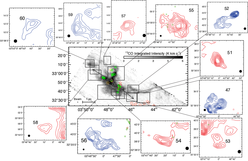
Figure 10.— CPOCs in Area VI. Lines with arrow show the extent of the B5-IRS molecular outflow lobes, including the new extensions reported here. The rest is the same as in Figure 5.

However, the recent studies of Brunt et al. (2009) and Padoan et al. (2009) have claimed that even in a region full of outflows like NGC 1333 the turbulence is mostly driven by large-scale mechanisms that originate outside the cloud (e.g., supornova explosion) and that small-scale driving of turbulence inside molecular clouds may only be somewhat important in regions close to outflows. Brunt et al. and Padoan et al. use the principal component analysis (PCA) method and the velocity coordinate spectrum (VCS) method, respectively, on CO line maps of NGC 1333 to study the turbulent energy spectrum and derive a driving length of turbulence in this region. The results of both studies, from analysis of the COMPLETE ¹³CO(1-0) map, imply that turbulence is not driven at scales smaller than the size of NGC 1333. Padoan et al. (2009) argue that this suggests the turbulent driving is primarily from sources outside the region rather than outflows within NGC 1333. It could very well be that the large-scale shells driven by stellar winds we find throughout the Perseus cloud complex are the source of this large-scale driving mechanism (Arce et al., in preparation). Brunt et al. (2009) also analyze the C¹⁸O(1-0) data of the same region, and they point out that there is evidence for turbulence driving at scales of approximately 0.3 to 0.7 pc (assuming a distance to NGC 1333 of 250 pc) which could be due to outflows. We caution that in both of these studies, in order to reach their conclusions, they have to compare the analysis they performed on the observed data to a similar analysis using synthesized maps from numerical simulations. In these simulations turbulence is driven in Fourier space using a field of random Gaussian fluctuations with a limited range of wave numbers. Although this is a reasonable approximation that facilitates running the numerical simulation, it is not how turbulence is driven in nature. Comparing real molecular clouds to simulations that use uniform turbulence driving might provide some information on the driving scale, but it is probably not the whole story. As we discussed above, the total outflow energy input rate in the six regions of star formation is enough to drive turbulence. If outflows are not important in driving the observed turbulence, then this raises the question of where does all the outflow energy go. It is clear these two studies are not the final word on this issue, and further studies are needed to fully understand the process of outflow-generated turbulence.

Table 4Regions of Active Star Formation in Perseus

Name	SE corner		NW corner		Vel. Range
	R.A.	Dec	R.A.	Dec	min.	max.
	(J2000)		(J2000)		(km s-1)
L1448	03:25:42	30:37:40	03:23:55	30:53:00	3.3	6.3
NGC1333	03:31:05	30:33:50	03:26:52	31:59:40	5.2	10.2
B1-Ridge	03:33:07	30:30:50	03:30:19	30:53:40	4.6	8.5
B1	03:34:00	30:54:30	03:31:33	31:19:50	4.8	8.7
IC348	03:46:02	31:52:50	03:43:06	32:29:40	6.5	11.4
B5	03:51:05	32:30:20	03:44:07	33:28:40	8.7	11.4

5.2.2 Outflows and Star Formation Efficiency

Recent three-dimentional numerical simulations show that outflows from a cluster of protostars can easily sustain the supersonic turbulence in the surrounding gas (Nakamura & Li 2007, herafter NL07; Carroll et al. 2009). In particular, the results of NL07 show that the turbulence in an isolated cluster-forming region of about two parsecs in size, fed by the energy and momentum injected by bipolar outflows, can maintain the region close to dynamic equilibrium. In this quasi-equlibrium state, infall and outflows motions are approximately equal, but there is a net flux of mass towards the bottom of the potential well. This results in a slower collapse, compared to the global free-fall time, and only a few percent of the total gas mass is converted into stars within a free-fall time. Different runs by NL07 with differing outflow strengths show that the star formation rate per free-fall time decreases with increasing average outflow strength. Their study shows that more powerful outflows result in an increase in the turbulence in the gas, which then leads to a delay of the gravitational collapse and, consequently, a lower star formation efficiency per free-fall time.

Table 5Physical Parameters of Active Star Forming Regions in Persesus

Name	$M_{reg}$	$R_{reg}$	$\Delta v$	$T_{ex}$	$v_{esc}$	$E_{grav}$	$E_{turb}$	$t_{diss}$	$L_{turb}$
	(M☉)	(pc)	(km s-1)	(K)	(km s-1)	($10^{46}$ erg)	($10^{45}$ erg)	($10^{5}$ yr)	($10^{32}$ erg s-1)
L1448	150	0.6	1.9	10	1.5	0.3	2.9	2.6	3.6
NGC 1333	1100	2.0	2.2	13	2.2	5.2	28.8	5.7	15.9
B1-Ridge	210	0.7	1.9	13	1.6	0.5	4.1	3.1	4.1
B1	430	0.9	2.1	13	2.0	1.8	10.2	2.9	11.2
B5	420	1.4	1.5	12	1.6	1.1	5.1	7.6	2.1
IC 348	620	0.9	1.8	15	2.4	3.7	10.9	3.0	11.4

Here we investigate whether there is any relationship between the star formation efficiency and the total outflow strength in different star-forming regions in the Perseus cloud. We use the c2d catalog of young stellar objects (Evans et al. 2009) to search for the total number of young stars in each of the six different star-forming regions in Perseus studied here (see Table 4 and Figure 1). The total number of YSOs within the area of each region, as well as the fraction of those that are embedded (i.e., Class 0 and I) sources, are shown in Table 8. For each region, we calculate the current star formation efficiency ($SFE$) using $SFE=M_{YSO}/(M_{reg}+M_{YSO}+f*M_{flow})$, where $M_{YSO}$ is the total mass of young stellar objects within the region’s boundaries. We assume an average YSO mass of 0.5 M_☉, as in Jørgensen et al. (2008) and Evans et al. (2009). The mass of the gas in the region is given by $M_{reg}$ (see Table 5), and $f*M_{flow}$ is the mass ejected (or lost) from the region by outflows and other mechanisms. The observed total outflowing mass is given by $M_{flow}$ (see Table 6) and $f$ is a correction factor accounting for mass no longer visible (e.g., from previous outflow events, due to dissociation, etc.). It is difficult to obtain a precise estimate of $f$, but we think that a reasonable estimate lies in the range of 2 to 10, depending on the age of the star forming region (see below).

A cloud with a constant star formation rate will exhibit a higher star formation efficiency as the cloud evolves, since more of the cloud gas will be transformed into stars. In fact, the results of NL07 show that independent of average outflow strength, as soon as the first stars are formed, the SFE increases approximately linearly with time. In addition, regions with different free-fall times (and the same turbulent energy) will collapse at different rates and thus will exhibit different values of the current SFE (even for clouds of the same age). We therefore need to take into consideration the length of time that the region has been forming stars and its free-fall time in order to investigate whether the star formation efficiency of different regions depends on the outflow strength. For this purpose, we define the “normalized” star formation efficiency, $SFE_{n}\equiv SFE*(t_{ff}/\tau_{SF})$, where $t_{ff}$ is the free-fall timescale of the region (see above and Table 8), and $\tau_{SF}$ is the time the region has been forming stars (i.e., the region’s age).

Table 6Total Outflow Mass, Momentum, Energy and Luminosity in Star-Forming Regions

Name	$M_{flow}$	$P_{flow}$	$E_{flow}$	$L_{flow}$
	(M☉)	(M☉ km s-1)	($10^{44}$ erg)	($10^{32}$ erg s-1)
L1448	1.0 / 5	3.1 / 21.7	1.2 / 12	8
NGC1333	5.0 / 25	17.4 / 121.8	6.9 / 69	44
B1-Ridge	1.1 / 5.5	3.2 / 22.4	1.0 / 10	6
B1	1.5 / 7.5	6.2 / 43.4	3.1 / 31	20
IC348	4.2 / 21	7.7 / 53.9	1.5 / 15	10
B5	12.8 / 64	22.3 / 156.1	4.1 / 41	26

Table 7Quantitative Assessment of Outflow Impact on Star-Forming Regions

Name	$E_{flow}/E_{turb}$	$r_{L}=L_{flow}/L_{turb}$	$E_{flow}/E_{grav}$	$M_{esc}\tablenotemark{a}$ [M☉]	$M_{esc}/M_{c}$
L1448	0.41	2.1	0.40	15	0.10
NGC1333	0.30	3.4	0.17	76	0.07
B1-Ridge	0.24	1.5	0.20	14	0.07
B1	0.30	1.7	0.17	21	0.05
IC348	0.14	0.8	0.04	23	0.04
B5	0.80	12.4	0.37	98	0.23

Studies of the population of young stars in IC 348 (Luhman et al. 2003; Muench et al. 2007) and NGC1333 (Lada et al. 1996; Wilking et al. 2004) indicate that these two clusters have significantly different ages of about 2-3 Myr and about 1 Myr, respectively. Here we will assume an age of 2.5 Myr for IC 348 and 1 Myr for NGC 1333. For the other clumps in Perseus we use the fraction of Class I sources in the region to estimate their age. Assuming that star formation has been approximately constant, then the fraction of embedded protostars in a region can provide a rough relative lifetime of the star formation process in the clump. In IC 348 and NGC 1333 the fraction of Class I sources is 10% and 32%, respectively (see Table 8), consistent with the age difference between these two clusters (Jørgensen et al. 2006). Similar to NGC 1333, all the other star-forming regions in Perseus, except L1448, have a fraction of Class I sources of about 30% to 50% and their YSO populations include evolved young stars (with ages of about 1 Myr) in the late Class II stage —as derived from the sources’ bolometric temperature and spectral index (see Evans et al. 2009 for more detail). We thus assume that regions B5, B1, and B1-Ridge also have an age of about 1 Myr. In L1448 all the YSOs are Class I sources, which suggests that this region is significantly younger than the rest. We assume the age of L1448 is 0.5 Myr, the average lifetime of the Class I stage as derived by Evans et al. (2009). We also use the relative populations of embedded protostars to obtain a rough estimate of $f$, the correction factor accounting for mass no longer visible in the $SFE$ equation above. The value of $f$ in L1448 should be between 1 and 2, while $f\sim 3$ should be a reasonable estimate for B5, B1, B1-Ridge and NGC 1333. In IC 348 star formation has been taking place for a longer time ,and thus use $f=8$ for this region.

The values of the normalized SFE in the different star-forming regions of Perseus, shown in Table 8, range from 0.3% to 3.4%, with B5 and NGC1333 showing the smallest and largest values, respectively. From the study of NL07 we expect a lower $SFE_{n}$ for regions with stronger outflows. We use the ratio of the total outflow luminosity to the energy rate needed to maintain the turbulence in the gas ($r_{L}$, in Table 7) as a way to quantify the outflow strength and their impact on the cloud’s turbulence. Clouds with $r_{L}>1$ harbor outflows that input enough energy into the surrounding gas to maintain the observed turbulence in the cloud. Assuming the magnetic field strength is approximately the same for all clouds in Perseus, then according to NL07, the outflow-driven turbulence should be the dominant source for variations in the SFE. We would therefore expect clouds with a high $r_{L}$ to have a low $SFE_{n}$. However, our results do not show a clear dependence of $SFE_{n}$ with $r_{L}$ (see Figure 11). We see that B5 (the region with the largest $r_{L}$) exhibits the lowest value of $SFE_{n}$ but otherwise there is no correlation between $r_{L}$ and $SFE_{n}$.

It is hard to draw any strong conclusion from our results probably due to the large uncertainties in estimating $SFE_{n}$. The number of stars formed in the cloud (a number essential for estimating SFE) is uncertain as we only include YSOs in the c2d catalog that are within the regions defined by us, and thus we are not accounting for stars formed in the cloud but that have since moved away from the defined region. In addition, the list of young stars is not 100% complete as, among other things, it does not include pre-main sequence stars that do not have a detectable infrared excess (see Evans et al. 2009 more details). Moreover, age estimates for the star-forming regions, as well as the free-fall timescales are probably uncertain within a factor of two or so. Given the large uncertainties in $SFE_{n}$, the small size of the sample and the limited range in values of the total outflow momentum and $r_{L}$ among all regions, it is of no surprise that we do not find a significant correlation between $SFE_{n}$ and outflow strength, even if such correlation exists. Clearly, a larger sample of star-forming regions with accurate age and SFE estimates is needed in order to study this further.

5.2.3 Disruption of the cloud by outflows?

It has also been proposed that outflows can have a disruptive impact on their clouds (e.g., Arce & Goodman, 2002a). One way to estimate the disruptive effects of outflows on clouds is by comparing the outflow energy with the cloud’s gravitational energy. From Table 7 it can be seen that the total kinetic energy of the outflows is only a small fraction (between 4 and 40%) of the gravitational binding energy of each region. From this simple analysis, it appears that for most regions, outflows do not have the necessary energy to significantly disrupt their cloud. Another way to assess the potential disruptive effect of outflows on clouds is using the “escape mass” ($M_{esc}$) of the region, defined as the mass that could potentially be dispersed by the outflows if we assume that the total current outflow momentum is used to accelerate a total gas mass of $M_{esc}$, through conservation of momentum, to the cloud sub-region’s escape velocity (i.e., $M_{esc}=P_{flow}/v_{esc}$). We note that in all regions the current total outflow mass is lower than $M_{esc}$ only by factors of 1.5 to 3.5, so it is possible that the current outflows could eventually entrain as much mass as $M_{esc}$. From our analysis we see that outflows in the active star-forming regions of Perseus currently have enough momentum to potentially disperse only 4% to 23% of the mass in their respective regions (see Table 7).

Table 8Star Formation Efficiency in Different Regions of the Perseus Molecular Cloud

Region	No.	No.	SFE	$t_{ff}$	$\tau_{SF}$	$SFE_{n}$
Name	YSOs	Embedded	(%)	Myr	Myr	(%)
L1448	5	5 (100%)	1.5	0.31	0.5	0.9
NGC1333	125	40 (32%)	4.9	0.69	1	3.4
B1-Ridge	11	3 (27%)	2.4	0.33	1	0.8
B1	19	10 (52%)	2.1	0.33	1	0.7
IC348	154	16 (10%)	9.0	0.28	2.5	1.0
B5	5	3 (60%)	0.4	0.65	1	0.3

It appears that current outflows do not have enough strength to cause serious impact to the integrity of their cloud. However, it is possible that the estimated momentum from our observations of the current outflows is just a fraction of the total momentum from all outflow events from all protostars that form throughout the entire life of the cloud. As discussed above, the observed current molecular outflows most probably have ages of about 0.2 Myr or less. In addition, most of the star forming regions in Perseus are only $\sim 1$ to 3 Myr old, but molecular clouds have lifetimes of about 3 to 6 Myr (e.g., Evans et al. 2009). If star formation and outflow production continues at a roughly constant rate (or increases with time), it is then possible that the total momentum injected by outflows into the gas, throughout the entire history of the star-forming region could be considerably larger that what we estimate from our limited snapshot of the cloud. If, for example, the total outflow momentum injected over the lifetime of the cloud turns out to be a factor of ten more than the current observed outflow momentum, this would then imply that outflows could seriously disrupt the three least massive regions in our study (i.e, L1448, B1-Rdige, and B5), as outflows could potentially disperse 70% or more of the current mass in these regions. In this scenario, outflows in the other three region would be able to potentially dispersed 40 to 70% of the gas. A loss of 40% of the original mass may still cause some significant damage to the integrity of the clump as it will be left with a gravitational binding energy that is 36% of the original value (assuming the cloud size stays the same). We conclude that outflows may disperse some gas from their parent cloud, yet unless the amount of momentum that outflows inject into their surroundings throughout the entire lifetime of the cloud is more than a factor of ten compared to current outflow momentum estimates, outflows cannot fully disrupt their parent clouds.

The theoretical work of Matzner & McKee (2000) studied the combined effects of many outflows on the gas of clumps forming clusters of low-mass stars. Their results predict about 30% to 50% of the mass will be turned into stars, while the rest (i.e., 50% to 70%) of the gas in the cluster-forming region will be ejected by outflows. For these theoretical results to be consistent with our findings, outflow momentum injection throughout the entire lifetime of the cloud would have to be more than a factor of 10 of the current outflow momentum for all studied regions in Perseus to experience (at least) a 50% gas dispersion due to outflows by the end of cloud’s lives. It seems very unlikely that in all cases outflows alone will disperse such a high fraction of the cluster-forming gas. A more plausible scenario would be that outflows help disperse a fraction of their surrounding gas and other mechanisms, such as dispersion by stellar winds and erosion produced by radiation, help dissipate the rest of the gas that does not end up forming stars —thereby producing the star formation efficiencies ($\sim 10\%$ to 30%) observed in clusters (e.g., Lada & Lada 2003).

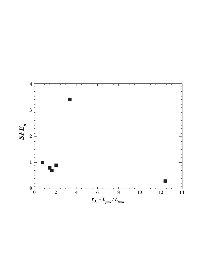
Figure 11.— Normalized star formation efficiency as a function of $r_{L}$ for different regions of star formation in Perseus. No error bars are shown as it is hard to estimate accurate $1-\sigma$ uncertainties for these points. The uncertainties in the values of $SFE_{n}$ and $r_{L}$ could easily be a factor of two (or even more).

We note that the discussion above only relates to the impact of outflows on their cloud at scales of about 1 pc, and it does not pertain to the impact of outflows on their host cores. Our observations probe regions with size of $\sim 1$ to 4 pc and density of $\sim 10^{3}$, which are are considerably more extended and less dense than the cores in Perseus, which have an average radius and density of $\sim 0.04$ pc and $\sim 10^{5}$ cm^-3 (Enoch et al. 2008). The results presented here do not rule out that outflows can be a major player in the mass loss process in cores (as reported by, e.g., Fuller & Ladd 2002; Arce & Sargent 2005, 2006).

6. Summary and Conclusions

A survey of all the high velocity outflow features was conducted for Perseus using ¹²CO and ¹³CO molecular line maps from the COMPLETE Survey in order to gain a better understanding of how outflows effect their host cloud complex over large areas. Our $\sim 6.25\arcdeg\times 3\arcdeg$ maps cover almost the entire Perseus molecular cloud complex which allows us to search for outflows throughout the extent of the cloud and not just in the immediate surrounding of active star-forming regions as in most previous studies. We utilize a novel way to search for outflows using 3D visualization of the molecular cloud in position-position-velocity space. Rendering the molecular line data this way shows high-velocity blobs as clearly visible spikes that stick out from the general cloud gas distribution. Using this technique we detected previously known outflows and new outflow candidates. Our survey results show that most molecular outflows in Perseus concentrate close to a few groups and clusters of protostars, and there are vast areas of the cloud where there is little or no molecular outflow activity. We compiled a list of 60 COMPLETE Perseus Outflow Candidates (CPOCs) that lie across the entirety of Perseus, with most of them found around the periphery of, and in between, active star forming regions. We identified a few of these CPOCs as being previously unknown extensions of previously known outflows. In particular, we find new extensions to the well-known B5-IRS1 outflow which now has a total projected length of $\sim 1\arcdeg$ (or about 4.4 pc).

The newly identified candidate outflows more than double the amount of molecular outflow mass, momentum and kinetic energy in Perseus. Outflows have considerable impact on the environment immediately surrounding localized regions of active star formation, but lack the energy needed to feed the observed turbulence in the entire Perseus cloud complex, even with the increase in outflowing material found by our study. We propose there must be another energy source, in addition to collimated outflows from protostar, responsible for maintaining the turbulence on a global cloud scale. We leave the discussion on spherical winds from young stars as a possible source of turbulence in Perseus for a subsequent paper.

We compared the total outflow momentum, energy and power in the different local star-forming regions —areas of active star formation with numerous outflows and sizes 1 to 4 pc— with the energetics of the host cloud sub-region to quantitatively assess the outflow impact on their surroundings. Our results indicate that outflows have enough power (or can contribute substantially) to maintain the turbulence in their local environment.

The numerical simulations of Nakamura & Li (2007) show that outflow-driven turbulence can affect the star formation efficiency in their parent cluster-forming clump and we use our data (together with data from the literature) to investigate if this is the case in Perseus. We detect no correlation between star formation efficiency and outflow strength, but the large uncertainties in these values prevent us from reaching any definitive conclusion on this issue.

Our quantitative assessment of the impact of current outflows on Perseus indicates that outflows have the potential to disperse and unbind some mass from the cloud. The current outflow energy and the amount of material that current outflows can potentially unbind, compared to the total mass of the region, is not enough to cause major disruptions to the cloud. The total outflow momentum injection throughout the entire lifetime of the cloud would have to be more than an order of magnitude greater than the detected current outflow momentum in order for gas dispersion by outflows to cause a serious impact to the integrity of their host cloud. We argue that, in addition to collimated outflows from young stars, other mechanisms of cloud dispersal are needed to explain the low star formation efficiency in clusters.

Appendix A Description of CPOCs

Here we discuss our findings for each of the six areas we divided the Perseus cloud complex into (as shown in Figure 1).

A.1. Area I

Area I is the westernmost part of the Perseus cloud complex, which includes the L1448 and L1455 dark clouds. L1448 is a relatively small ($\sim$0.5 deg², 150 M_☉) and isolated star forming region centered around $\alpha=03^{h}25^{m}30^{s}$, $\delta=31\arcdeg 45\arcmin$. This region harbors five embedded (Class 0 and Class I) protostars, and no Class II or III sources (Evans et al., 2009). The protostars in L1448 power well-known outflows that have been observed across multiple wavelengths (Bachiller et al., 1990a; Bally et al., 1997; Wolf-Chase et al., 2000; Eislöffel, 2000; Walawender et al., 2005a; Kwon et al., 2006; Tobin et al., 2007; Davis et al., 2008). The L1455 region lies about one degree southeast of L1448, and it is only partially included in the lower edge of our CO maps. L1455 harbors protostars that power previously-observed molecular outflows, but with our limited map of the region we only detect the outflow that has a southeast-northwest axis and is associated with L1455-IRS4 (Bally et al., 1997; Jørgensen et al., 2006).

We detected four new candidate outflow features in the periphery of the L1448 region (CPOCs 1 to 4) and one in the area between L1448 and L1455 (CPOC 5). These high-veolcity features were marked as candidate outflows because they show “typical” outflow spectra with low-intensity high-velocity wings and they lie in close proximity to an active region of star formation with multiple HH objects in their surroundings. CPOCs 1, 2 and 3 lie west-northwest of the center of the L1448 cluster of protostars and lie close to several HH objects in this region (i.e., HH194 and HH268). The morphology and position of CPOCs 1 and 2 (see Figure 5) strongly suggest that they are extensions of the outflow presumably powered by IRAS 03220+3035, also known as L1448-IRS1 (Bally et al., 1997). CPOC 3 is redshifted and lies about 10′ north of L1448, and within 3′ of two groups of HH objects. CPOC 4 is blueshifted and lies less than 10′ southwest of L1448-IRS1. The position and velocity of this CPOC are not consistent with it being powered by L1448-IRS1, but given its close proximity to the group of embedded protostars in L1448, is highly probable that this CPOC is powered by any one of these forming stars. CPOC 5 is blueshifted and lies just south of the c2d YSO candidate SSTc2dJ032519.52+303424.2. It is not clear whether this YSO candidate or any of the protostars in L1448 or in L1455 is the powering source of this CPOC.

A.2. Area II

This area mostly includes the NGC 1333 cluster and its surroundings. NGC 1333 is presently the most active star forming region in Perseus, covering $\sim$1 deg² with a total gas mass of 1100 M_☉. Located at the western part of the cloud complex, it contains two contiguous young stellar clusters that include about 275 members ranging in age from protostars to pre-main-sequence stars (i.e., Class 0 to III sources) (Lada et al., 1996; Rebull et al., 2007; Gutermuth et al., 2008). NGC 1333 has also been surveyed for outflows at different wavelengths (Bally et al., 1996a; Yan et al., 1998; Knee & Sandell, 2000; Davis et al., 2008; Hatchell & Dunham, 2009). This region contains several identified and well-studied molecular outflows including that of IRAS 4A, IRAS 2A, IRAS 2B and HH7-11 (Bachiller et al., 2000; Knee & Sandell, 2000; Jørgensen et al., 2004; Choi et al., 2006; Jørgensen et al., 2007a). We detect high-velocity CO emission at positions coincident with these outflows, however due to the relatively low resolution of our map we cannot disentangle individual outflows in the central core of the NGC 1333 cluster —the area within $\alpha$ from about $03^{h}28^{m}30^{s}$ to $03^{h}29^{m}30^{s}$ and within $\delta$ from about $31\arcdeg 10\arcmin$ to $31\arcdeg 30\arcmin$ (J2000), studied previously by Knee & Sandell (2000) and Hatchell & Dunham (2009).

Although NGC 1333 has been very well surveyed for molecular outflows in its central clustered region, few studies have examined the cluster’s outskirts. We identify new candidate outflows all around the outer parts of NGC 1333 as well as in the gas east of the cluster, between NGC 1333 and B1, and near the Per 6 protostellar aggregate south of NGC 1333 (Rebull et al., 2007). In the western edge of the cluster lies CPOC 6, a high-velocity redshifted candidate outflow close to HH 338 (see Figure 6). CPOC 7 is a blueshifted outflow candidate south of the main cluster core, and close to several HH objects and YSO candidates (the closest being SSTc2dJ032834.49+310051.1). CPOC 8, located south of NGC 1333, lies between three c2d YSO candidates and two HH objects (HH 750 and HH 743), but it is not clear which of these nearby young stars is the source of this elongated outflow candidate. In the west-southwest outskirts of the NGC 1333 core lies CPOC 9, a redshifted outflow candidate that coincides with the position of at least five HH objects (and H₂ knots) and two YSO candidates (SSTc2dJ032832.56+311105.1, and SSTc2dJ032837.09+311330.8). CPOCs 13 and 10 lie to the immediate north and northwest of the cluster core, respectively. The most likely powering source of CPOC 10 is SSTc2dJ032844.09+312052.7, which lies on the southeast corner of this outflow candidate. CPOC 13 is coincident with at least six HH objects and H₂ knots and one of the multiple sources just south of this CPOC could be its powering source. CPOCs 11 and 12 are redshifted and blueshifted, respectively, and lie very close to each other. There are no known YSOs right at the position between these two CPOCs, so it is likely that each outflow candidate is associated with a different powering source. From the distribution of the high-velocity gas in relation to the position of the various YSO candidates in the region, STTc2dJ032834.53+310705.5 seems to be the most likely candidate for being the powering source of CPOC 11, while SSTc2dJ032843.24+311042.7 is the most likely candidate source of CPOC 12. CPOCs 14 and 15 are another pair of red and blue outflow candidates that lie near HH 757A/B and HH 426 as well as near two c2d YSO candidates in the southern outskirts of the NGC 1333 cluster. In this region we also detect high-velocity redshifted emission located at the same position as IRAS 03254+3050, just south of the main cluster core. We do not include this in the list of CPOCs as this high-velocity gas is coincident with the high-velocity CO(3-2) emission recently reported by Hatchell & Dunham (2009). We note that the prevalence of redshifted CPOCs north and west of NGC 1333 is due to the fact that there is intervening gas at blueshifted velocities with respect to the central velocity of NGC 1333 that hampers our ability to detect outflow-related blueshifted emission.

In the southern edges of the cluster core, and coincident with HH 18A and H₂ knot 25 in Davis et al. (2008), we find the redshifted CPOC 16. It has a northwest-southeast elongation which indicates it could be part of an outflow with its origin near the cluster center. CPOC 17 is a high-velocity redshifted blob east of the cluster core. Its relatively high mass and size implies that it is probably the result of the impact of multiple outflows on the surrounding molecular gas. This picture is supported by the fact that there are multiple YSO candidates and HH objects (including the HH flows HH 497 and HH 336) coincident with CPOC 17. On the northeastern outer limits of the main NGC 1333 cluster, and coincident with HH 764, lies CPOC 18. About five arcminutes east of CPOC 18, and close to HH 497, lies CPOC 20. It is very probable that this CPOC is the extension of one of the many molecular outflows originating in NGC 1333. To the north of NGC 1333 we also find CPOC 19, which has a highly elongated morphology, typical of collimated outflow lobes, and lies close to SSTc2dJ032923.48+313329.5 (IRAS 03262+3123). CPOC 21, in the eastern outskirts of the main part of the NGC 1333 cluster, has a west-east elongation and it is coincident with HH 767. This HH object is part of a chain of HH objects that presumably are part of the same east-west parsec-scale flow, composed of HH 348, HH 349, HH 766, and HH 767 (Walawender et al. 2005). A candidate powering source for this CPOC is SSTc2dJ033024.08+311404.4, which lies at the eastern edge of the redshifted gas. Halfway between the B1 and NGC 1333 star forming regions we find CPOCs 23, 25 and 27. It is hard to tell whether this chain of high-velocity blueshifted blobs are related (or are driven by different sources) and whether they are part of an outflow originating in NGC 1333 or B1. Lastly, in this region we find CPOC 22, a blueshifted candidate outflow that most likely is driven by one of the protostars in the recently discovered Per 6 aggregate (Rebull et al., 2007).

A.3. Areas III and IV

This part of the Perseus cloud complex includes the Barnard 1 (B1) dark cloud, the ridge southwest of B1 (the B1-Ridge), and the area just east of B1 (see Figure 1). B1 and the B1-Ridge are two regions of active star formation that have been well surveyed in multiple wavelengths (Bachiller & Cernicharo, 1984; Bachiller et al., 1990b; Yan et al., 1998; Jørgensen et al., 2006; Rebull et al., 2007; Hiramatsu et al., 2010), and they are host to multiple known outflows including B1-a,b,c, and the outflows powered by IRAS 03304+3100, IRAS 03295+3050, IRAS 03292+3039, and IRAS 03282+3035 (Bachiller et al., 1991; Hirano et al., 1997; De Gregorio-Monsalvo et al., 2005; Walawender et al., 2005b; Jørgensen et al., 2006; Davis et al., 2008).

We identify three possible new outflows (or extension to previously known outflows) in the outer parts of the B1-Ridge (CPOCs 24, 26, 28) and eight located primarily around the periphery of the central B1 region (CPOCs 29 to 36) (see Figures 7 and 8). We mostly detect redshifted CPOCs in this region as there is a cloud along the same line of sight, at blueshifted velocities with respect to the B1 clump, that hinders our ability to detect outflow-related high-velocity blueshifted emission around B1. Some of the CPOCs in this area (e.g., CPOCs 24, 26, 28) are probably extensions of outflows originating in the core of B1 and the B1-Ridge, just like the many HH objects recently found in the periphery of these star-forming regions (Walawender et al., 2005b). Other CPOCs found here could be new outflows associated with young stars that lie outside the central core of B1 (e.g., CPOCs 31, 34, 35, and 36). With the relatively low resolution of our map it is difficult to concretely determine the driving source for candidate outflows in this region of high protostellar density. We still give possible candidate sources (based on the proximity of the CPOC to a candidate YSO) in Table 1. Our discovery of new outflow candidates in the outer limits of these clusters show yet another example of how typical studies usually overlook the periphery of active star forming regions, and the need for studies that encompass a larger area in order to obtain a complete census of the outflows in the cloud.

A.4. Area V

The western part of Area V contains a scantly studied region of the Perseus molecular cloud complex that lies between the B1 dark cloud and IC 348 cluster, and the eastern end includes the region surrounding the young stellar cluster IC 348 (see Figure 9). The region east of B1 and west of IC 348 does not contain any major clusters or groups of young stars, but it does include signposts of star formation. It is host to three, poorly known, dark clouds (i.e., L1468, B3 and B4), several high-extinction cores (Wood et al., 1994), a few c2d YSO candidates (Evans et al., 2009), and IRAS sources (Ladd et al., 1993). This area of Perseus is also the location of a warm shell of dust most likely the result of an H II region associated with the early-B star HD 278942 that lies behind the cloud (Andersson et al., 2000; Ridge et al., 2006b).

We identify eight new outflow candidates in this region (CPOCs 37 to 44), most of which are clustered about 1 degree to the west of IC 348. CPOC 39 has a very elongated morphology, similar to the structure of a collimated outflow lobe, and it is located between the c2d YSO candidates SSTc2dJ033915.81+312430.7 and SSTc2dJ034001.49+311017.3. Although the latter YSO candidate is closer to CPOC 39, either of these two young stars could be the powering source of this high-velocity gas. We also find two sets of adjacent red and blue CPOCs that seem to pair to form two candidate bipolar flows. One of them is comprised of CPOC 40 and 42, and it is very close to IRAS 03363+3027 (see Figure 9). Although the IRAS source does not lie in the center of the two CPOCs, the uncertainty in its position (i.e., an ellipse with a major axis of 43″, minor axis of 13″, and a PA=73°) is large enough that it is feasible that IRAS 03363+3207 could be the source of this candidate bipolar flow. The other, weaker, candidate bipolar outflow is comprised of CPOC 37 and 38 (see Figure 9). We cannot assign a possible source to this candidate outflow as there are no known YSOs in this area. One possible reason for the lack of YSO candidates in the northwestern part of this region (where we find CPOCs 40 to 43, and CPOCs 37 and 38) is the fact that this area was not covered by the c2d Spitzer IRAC observations (Jørgensen et al., 2006). Wood et al. (1994) identified a few cores just to the north of these candidate outflows and outside the northern edge of our CO map. Hence, it may be possible that the fast moving gas observed in the northwest part of Area V (i.e., CPOCs 37, 38, 41, 43) is powered by undetected YSOs in the northern parts of Perseus. We find CPOC 44 about 30′ southwest of the main IC 348 cluster, among a group of c2d YSO candidates (see Figure 9). Any of these young stars could be the powering source of this high-velocity feature.

IC 348, at the eastern edge of Area V, consists of two portions: the northeast part which contains the well known cluster of young stars; and the southwest part (about 10′ southwest of the center of the main cluster) which harbors a more recent burst of star formation activity (Herbst, 2008). The young cluster located in the northeast portion of the region has been recently studied by a number of authors (Luhman et al., 2003; Muench et al., 2007), which show that the few hundred members of this cluster have a wide spread in age, ranging from Class I to Class III sources. This portion of the region contains no known molecular outflows, and is home to a B5 star (HD 281159) that powers a reflection nebula seen both in the optical and NIR. The region to the southwest of the main cluster (also known as IC 348-SW; Tafalla et al. 2006) contains high-density gas, has a higher extinction and harbors more embedded protostars than the rest of IC 348. It also contains a number of HH objects and a few well-known molecular outflows (Eislöffel et al., 2003; Tafalla et al., 2006; Walawender et al., 2006), including HH 211 (McCaughrean et al., 1994; Gueth & Guilloteau, 1999).

We identify 4 potential new molecular outflow candidates located just to the east of IC 348-SW: CPOCs 45, 46, 48, 49 and 50 (see Figure 9). In the northern portion of the main stellar cluster we also detect another candidate outflow, CPOC 46. All of these CPOCs lie in a region rich in c2d YSO candidates, however our CO maps lack the necessary angular resolution to confidently assign a powering source to each candidate outflow. One particular pair of high-velocity blobs is made of the red and blue CPOCs 48 and 49, which are located next to each other and might comprise the two lobes of a bipolar outflow. A candidate young star that could be the powering source of this candidate outflow is the nearby c2d YSO candidate SSTc2dJ034458.55+315827.1. In the IC 348-SW region we detect the high-velocity gas associated with HH 211 and other neighboring outflows, but we fail to detect any new outflows or outflow extensions.

A.5. Area VI

Area VI includes the Barnard 5 (B5) dark cloud, also known as L1471, located at the eastern end of the Perseus molecular cloud complex. The region has only a few young stellar objects, as revealed from infrared studies of the region (e.g., Beichman et al., 1984; Evans et al., 2009). The c2d Spitzer IRAC survey did not cover the entire B5 region thus there may be a few low-luminosity YSO candidates in the eastern part of B5 not detected by IRAS. The region is home to the well studied parsec-scale outflow from B5-IRS1 (Goldsmith et al., 1986; Fuller et al., 1991; Bally et al., 1996b; Yu et al., 1999).

In this region we identify two high-velocity features which we suggest are new extensions of the B5-IRS1 outflow (CPOCs 51 and 59). Yu et al. (1999) place the ends of each outflow lobe of the B5-IRS1 outflow at the position of V-shaped (i.e., bow-shaped) CO blobs at approximately $20\arcmin$ from the source, which they labeled C1 and C2. The redshifted CPOC 51 has an elongated structure, with a major axis that is coincident with the redshifted lobe of the B5-IRS1 outflow, and lies about $11\arcmin$ (or 0.8 pc at a distance of 250 pc) southwest of C2. The blueshifted CPOC 59 lies about $10\arcmin$ northeast of C1 and it is elongated in the direction towards B5-IRS1. The position, velocity and morphologies of the CPOCs 51 and 59 suggest they are part of the B5-IRS1 outflow and are associated with ejections that occur much earlier than those related to the C1 and C2 structures reported by Yu et al. (1999). With these new extensions, the B5-IRS1 outflow has a total projected length of about $1\arcdeg$ (4.4 pc), approximately 50% longer than previously thought. This finding implies that there could be many other molecular outflows that are much larger than previously thought (as shown for HH flows by, e.g., Reipurth et al. 1997). It is possible that a significant number of the CPOCs reported here are extensions of previously known outflows, but in most cases it is hard to assign a source to the high-velocity blob (as discussed above, in § 4.1)

In this region we also detect nine other new candidate outflow features: CPOCs 47, 52, 53, 54, 55, 56, 57, 58, and 60 (see Figure 10). The most massive and energetic of these are CPOCs 55 and 56 (see Table 1). We classify CPOC 56 as a candidate outflow as it: has velocities that are far enough from the cloud to be considered a genuine high-velocity feature (see Figure 4); it is within 5 to $10\arcmin$ of HH objects and a YSO; and it shows a velocity structure where the gas at higher velocities is further away from the cloud center (similar to the so-called “Hubble-law” in molecular outflows where the outflow velocity increases with distance from the source). CPOC 55 lies very close to the YSO B5-IRS4 as well as several HH objects (see Figure 10) and shows a clearly different structure from that of the cloud at redshifted velocities. CPOC 47 is located just to the north of IC 348 where there are a number c2d YSO candidates, and this candidate outflow is most probably associated with one of these sources rather than any of the sources in B5. CPOC 52 is a blob with relatively high-velocity blueshifted gas, significantly different from ambient cloud velocities (see Figure 4). CPOCs 53 and 54 have redshifted velocities and may be associated with HH 844 and IRAS 03439+3233 (also known as B5-IRS3). CPOC 57 is redshifted and is located about 10′ northeast of B5-IRS4, while CPOC 58 is located south of the blueshifted lobe of B5-IRS1 and it is not clear to which young star in the region it is associated with. CPOC 60 is located at the eastern edge of our map. We classify it as a candidate outflow because of its morphology and velocity structure.

References

- Andersson et al. (2000) Andersson, B.-G., Wannier, P. G., Moriarty-Schieven, G. H., & Bakker, E. J. 2000, AJ, 119, 1325
- Arce & Goodman (2001a) Arce, H. G., & Goodman, A. A. 2001, ApJ, 551, L171
- Arce & Goodman (2001b) Arce, H. G., & Goodman, A. A. 2001, ApJ, 554, 132
- Arce & Goodman (2002a) Arce, H. G., & Goodman, A. A. 2002, ApJ, 575, 911
- Arce & Goodman (2002b) Arce, H. G., & Goodman, A. A. 2002, ApJ, 575, 928
- Arce & Sargent (2005) Arce, H. G., & Sargent, A. I. 2005, ApJ, 624, 232
- Arce & Sargent (2006) Arce, H. G., & Sargent, A. I. 2006, ApJ, 646, 1070
- Arce et al. (2007) Arce, H. G., Shepherd, D., Gueth, F., Lee, C.-F., Bachiller, R., Rosen, A., & Beuther, H. 2007, in Protostars and Planets V, eds. B. Reipurth, D. Jewitt, and K. Keil, (University of Arizona Press: Tucson), 245
- Aspin et al. (1994) Aspin, C., Sandell, G. & Russell, A. P. G. 1994, A&AS, 106, 165
- Bachiller & Cernicharo (1984) Bachiller, R., & Cernicharo, J. 1984, A&A, 140, 414
- Bachiller & Cernicharo (1986) Bachiller, R., & Cernicharo, J. 1986, A&A, 168, 262
- Bachiller et al. (1990a) Bachiller, R., Martin-Pintado, J., Tafalla, M., Cernicharo, J., & Lazareff, B. 1990a, A&A, 231, 174
- Bachiller et al. (1990b) Bachiller, R., Menten, K. M., & del Rio Alvarez, S. 1990b, A&A, 236, 461
- Bachiller et al. (1991) Bachiller, R., Martin-Pintado, J., & Planesas, P. 1991, A&A, 251, 639
- Bachiller et al. (2000) Bachiller, R., Gueth, F., Guilloteau, S., Tafalla, M., & Dutrey, A. 2000, A&A, 362, L33
- Banerjee et al. (2007) Banerjee, R., Klessen, R. S., & Fendt, C. 2007, ApJ, 668, 1028
- Bally et al. (1996a) Bally, J., Devine, D., & Reipurth, B. 1996a, ApJ, 473, L49
- Bally et al. (1996b) Bally, J., Devine, D., & Alten, V. 1996b, ApJ, 473, 921
- Bally et al. (1997) Bally, J., Devine, D., Alten, V., & Sutherland, R. S. 1997, ApJ, 478, 603
- Bally & Reipurth (2001) Bally, J., & Reipurth, B. 2001, ApJ, 546, 229
- Beichman et al. (1984) Beichman, C. A., et al. 1984, ApJ, 278, L45
- Borkin et al. (2005) Borkin, M. A., Ridge, N. A., Goodman, A. A., & Halle, M. 2005, ArXiv Astrophysics e-prints, arXiv:astro-ph/0506604
- Borkin et al. (2007) Borkin, M., Goodman, A., Halle, M., & Alan, D. 2007, Astronomical Data Analysis Software and Systems XVI, 376, 621
- Borkin et al. (2008) Borkin, M., Goodman, A., Halle, M., & Alan, D. 2007, Astronomical Data Analysis Software and Systems XVII, 394
- Carroll et al. (2009) Carroll, J. J., Frank, A., Blackman, E. G., Cunningham, A. J., & Quillen, A. C. 2009, ApJ, 695, 1376
- Cernicharo & Reipurth (1996) Cernicharo, J. & Reipurth, B. 1996, ApJ, 460, L57
- Cernis (1990) Cernis, K. 1990, Ap&SS, 166, 315
- Choi et al. (2006) Choi, M., Hodapp, K. W., Hayashi, M., Motohara, K., Pak, S., & Pyo, T.-S. 2006, ApJ, 646, 1050
- Cunningham et al. (2009) Cunningham, A. J., Frank, A., Carroll, J., Blackman, E. G., & Quillen, A. C. 2009, ApJ, 692, 816
- Davis et al. (1999) Davis, C. J., Matthews, H. E., Ray, T. P., Dent, W. R. F., Richer, J. S. 1999, MNRAS, 309, 141
- Davis et al. (2008) Davis, C. J., Scholz, P., Lucas, P., Smith, M. D., & Adamson, A. 2008, MNRAS, 387, 954
- De Gregorio-Monsalvo et al. (2005) De Gregorio-Monsalvo, I., Chandler, C. J., Gómez, J. F., Kuiper, T. B. H., Torrelles, J. M., & Anglada, G. 2005, ApJ, 628, 789
- Dubinski et al. (1995) Dubinski, J., Narayan, R., & Phillips, T. G. 1995, ApJ, 448, 226
- Eislöffel (2000) Eislöffel, J. 2000, A&A, 354, 236
- Eislöffel et al. (2003) Eislöffel, J., Froebrich, D., Stanke, T., & McCaughrean, M. J. 2003, ApJ, 595, 259
- Enoch et al. (2006) Enoch, M. L., et al. 2006, ApJ, 638, 293
- Enoch et al. (2008) Enoch, M. L., Enoch, M. L., Evans, N. J., II, Sargent, A. I., Glenn, J., Rosolowsky, E., Myers, P. 2008, ApJ, 684, 1240
- Evans et al. (2009) Evans, N. J., et al. 2009, ApJS, 181, 321
- Falgarone et al. (1998) Falgarone, E., Panis, J.-F., Heithausen, A., Perault, M., Stutzki, J., Puget, J.-L., & Bensch, F. 1998, A&A, 331, 669
- Fukui et al. (1986) Fukui, Y., Sugitani, K., Takaba, H., Iwata, T., Mizuno, A., Ogawa, H., & Kawabata, K. 1986, ApJ, 311, L85
- Fuller et al. (1991) Fuller, G. A., Myers, P. C., Welch, W. J., Goldsmith, P. F., Langer, W. D., Campbell, B. G., Guilloteau, S., & Wilson, R. W. 1991, ApJ, 376, 135
- Fuller & Ladd (2002) Fuller, G. A., & Ladd, E. F. 2002, ApJ, 573, 699
- Gering (1999) Gering, D. 1999, Master’s Thesis, MIT
- Goldsmith et al. (1986) Goldsmith, P. F., Langer, W. D., & Wilson, R. W. 1986, ApJ, 303, L11
- Goodman et al. (1989) Goodman, A. A., Crutcher, R. M., Heiles, C., Myers, P. C., & Troland, T. H. 1989, ApJ, 338, L61
- Goodman & Arce (2004) Goodman, A. A., & Arce, H. G. 2004, ApJ, 608, 831
- Guenthner (2009) Guenthner, K. 2009, Master’s Thesis, Universität Leipzig
- Gueth & Guilloteau (1999) Gueth, F., & Guilloteau, S. 1999, A&A, 343, 571
- Gutermuth et al. (2008) Gutermuth, R. A., Myers, P. C., Megeath, S. T., Allen, L. E., Pipher, J. L., Muzerolle, J., Porras, A., Winston, E., Fazio, G. 2008, ApJ, 674, 336
- Hartigan et al. (2000) Hartigan, P., Bally, J., Reipurth, B., & Morse, J. A. 2000, in Protostars and Planets IV, eds. V. Mannings, A. P. Boss, S. S. Russell, (University of Arizona Press: Tucson), 841
- Hartmann et al. (2001) Hartmann, L., Ballesteros-Paredes, J., & Bergin, E. A. 2001, ApJ, 562, 852
- Hatchell et al. (2005) Hatchell, J., Richer, J. S., Fuller, G. A., Qualtrough, C. J., Ladd, E. F., Chandler, C. J. 2005, A&A, 440, 151
- Hatchell et al. (2007) Hatchell, J., Fuller, G. A., & Richer, J. S. 2007, A&A, 472, 187
- Hatchell & Dunham (2009) Hatchell, J., & Dunham, M., M. 2009, A&A, 502, 139
- Herbig & Jones (1983) Herbig, G. H. & Jones, B. F. 1983, AJ, 88, 1040
- Herbst (2008) Herbst, W. 2008, in Handbook of Star Forming Regions, Volume I: The Northern Sky, ed. Bo Reipurth, p.372
- Hiramatsu et al. (2010) Hiramatsu, M., Hirano, N., Takakuwa, S. 2010, ApJ, 712, 778
- Hirano et al. (1997) Hirano, N., Kameya, O., Mikami, H., Saito, S., Umemoto, T., & Yamamoto, S. 1997, ApJ, 478, 631
- Hirano & Taniguchi (2001) Hirano, N., & Taniguchi, Y. 2001, ApJ, 550, L219
- Hirota et al. (2008) Hirota, T. et al. 2008, PASJ, 60, 37
- Jørgensen et al. (2004) Jørgensen, J. K., Hogerheijde, M. R., Blake, G. A., van Dishoeck, E. F., Mundy, L. G., & Schöier, F. L. 2004, A&A, 413, 993
- Jørgensen et al. (2006) Jørgensen, J. K., et al. 2006, ApJ, 645, 1246
- Jørgensen et al. (2007a) Jørgensen, J. K., Johnstone, D., Kirk, H. & Myers, P. C. 2007a, ApJ, 656, 293
- Jørgensen et al. (2007b) Jørgensen, J. K., et al. 2007b, ApJ, 659, 479
- Kirk et al. (2006) Kirk, H., Johnstone, D., & Di Francesco, J. 2006, ApJ, 646, 1009
- Knee & Sandell (2000) Knee, L. B. G., & Sandell, G. 2000, A&A, 361, 671
- Kwon et al. (2006) Kwon, W., Looney, L. W., Crutcher, R. M., & Kirk, J. M. 2006, ApJ, 653, 1358
- Kutner & Ulich (1981) Kutner, M. L., & Ulich, B. L. 1981, ApJ, 250, 341
- Ladd et al. (1993) Ladd, E. F., Lada, E. A. & Myers, P. C. 1993, ApJ, 410, 168
- Lada & Fich (1996) Lada, C. J.. & Fich, M. 1996, ApJ, 459, 638
- Lada & Lada (1995) Lada, E. A. & Lada, C. J. 1995, AJ, 109, 1682
- Lada & Lada (2003) Lada, C. J. & Lada, E. A. 2003, ARA&A, 41, 57
- Lada et al. (1996) Lada, C. J., Alves, J., & Lada, E. A. 1996, AJ, 111, 1964
- Langer & Penzias (1993) Langer, W. D., & Penzias, A. A. 1993, ApJ, 408, 539
- Luhman et al. (2003) Luhman, K. L., Stauffer, J. R., Muench, A. A., Rieke, G. H., Lada, E. A., Bouvier, J. & Lada, C. J. 2003, ApJ, 593, 1093
- Mac Low (1999) Mac Low. M.-M. 1999, ApJ, 542, 169
- Margulis & Lada (1985) Margulis, M. & Lada, C. J. 1985, ApJ, 299, 925
- Margulis & Lada (1986) Margulis, M., & Lada, C. J. 1986, ApJ, 309, L87
- Masciadri & Raga (2001) Masciadri, E., & Raga, A. C. 2001, AJ, 121, 408
- Matzner (2007) Matzner, C. D. 2007, ApJ, 659, 1394
- Matzner & McKee (2000) Matzner, C. D., & McKee, C. F. 2000, ApJ, 545, 364
- McCaughrean et al. (1994) McCaughrean, M. J., Rayner, J. T., & Zinnecker, H. 1994, ApJ, 436, L189
- Muench et al. (2007) Muench, A. A., Lada, C. J., Luhman, K. L., Muzerolle, J. & Young, E. 2007, AJ, 134, 411
- Nakamura & Li (2007) Nakamura, F., & Li, Z.-Y. 2007, ApJ, 662, 395
- Norman & Silk (1980) Norman, C., & Silk, J. 1980, ApJ, 238, 158
- Padoan et al. (1999) Padoan, P., Bally, J., Billawala, Y., Juvela, M., & Nordlund, Å. 1999, ApJ, 525, 318
- Pineda et al. (2008) Pineda, J. E., Caselli, P., & Goodman, A. A. 2008, ApJ, 679, 481
- Raga et al. (2002) Raga, A. C., de Gouveia Dal Pino, E. M., Noriega-Crespo, A., Mininni, P. D., & Velázquez, P. F. 2002, A&A, 392, 267
- Rebull et al. (2007) Rebull, L. M., et al. 2007, ApJS, 171, 447
- Reipurth et al. (1997) Reipurth, B., Bally, J., & Devine, D. 1997, AJ, 114, 2708
- Reipurth & Bally (2001) Reipurth, B. & Bally, J. 2001, ARA&A, 39, 403
- Ridge et al. (2006a) Ridge, N. A., et al. 2006a, AJ, 131, 2921
- Ridge et al. (2006b) Ridge, N. A., Schnee, S. L., Goodman, A. A., & Foster, J. B. 2006b, ApJ, 643, 932
- Sargent (1979) Sargent, A. I. 1979, ApJ, 233, 163
- Stanke et al. (2000) Stanke, T., McCaughrean, M. J., & Zinnecker, H. 2000, A&A, 355, 639
- Stanke & Williams (2007) Stanke, T., & Williams, J. P. 2007, AJ, 133, 1307
- Sun et al. (2006) Sun, K., Kramer, C., Ossenkopf, V., Bensch, F., Stutzki, J., & Miller, M. 2006, A&A, 451, 539
- Tafalla et al. (2006) Tafalla, M., Kumar, M. S. N., & Bachiller, R. 2006, A&A, 456, 179
- Tafalla & Myers (1997) Tafalla, M., & Myers, P. C. 1997, ApJ, 491, 653
- Terquem et al. (1999) Terquem, C., Eislöffel, J., Papaloizou, J. C. B., & Nelson, R. P. 1999, ApJ, 512, 131
- Troland & Crutcher (2008) Troland, T. H., & Crutcher, R. M. 2008, ApJ, 680, 457
- Tobin et al. (2007) Tobin, J. J., Looney, L. W., Mundy, L. G., Kwon, W., & Hamidouche, M. 2007, ApJ, 659, 1404
- Ungerechts & Thaddeus (1987) Ungerechts, H., & Thaddeus, P. 1987, ApJS, 63, 645
- van Kempen et al. (2009) van Kempen, T. A., et al. 2009, A&A, 501, 633
- Walawender et al. (2004) Walawender, J., Bally, J., Reipurth, B. & Aspin, C. 2004, AJ, 127, 2809
- Walawender et al. (2005a) Walawender, J., Bally, J. & Reipurth, B. 2005a, AJ, 129, 2308
- Walawender et al. (2005b) Walawender, J., Bally, J., Kirk, H., & Johnstone, D. 2005b, AJ, 130, 1795
- Walawender et al. (2006) Walawender, J., Bally, J., Kirk, H., Johnstone, D., Reipurth, B., & Aspin, C. 2006, AJ, 132, 467
- Wilking et al. (2004) Wilking, B. A., Meyer, M. R., Greene, T. P., Mikhail, A., Carlson, G. 2004, AJ, 127, 1131
- Williams et al. (2003) Williams, J. P., Plambeck, R. L., & Heyer, M. H. 2003, ApJ, 591, 1025
- Wolf-Chase et al. (2000) Wolf-Chase, G. A., Barsony, M., & O’Linger, J. 2000, AJ, 120, 1467
- Wood et al. (1994) Wood, D. O. S., Myers, P. C., & Daugherty, D. A. 1994, ApJS, 95, 457
- Wu et al. (2004) Wu, Y., Wei, Y., Zhao, M., Shi, Y., Yu, W., Qin, S., & Huang, M. 2004, A&A, 426, 503
- Yan et al. (1998) Yan, J., Wang, H., Wang, M., Deng, L., Yang, J. & Chen, J. 1998, AJ, 116, 2438
- Yu et al. (1999) Yu, K. C., Billawala, Y., & Bally, J. 1999, AJ, 118, 2940
- Yu et al. (2000) Yu, K. C., Billawala, Y., Smith, M. D., Bally, J., & Butner, H. M. 2000, AJ, 120, 1974