Special-relativistic Smoothed Particle Hydrodynamics: a benchmark suite

Abstract

In this paper we test a special-relativistic formulation of Smoothed Particle Hydrodynamics (SPH) that has been derived from the Lagrangian of an ideal fluid. Apart from its symmetry in the particle indices, the new formulation differs from earlier approaches in its artificial viscosity and in the use of special-relativistic “grad-h-terms”. In this paper we benchmark the scheme in a number of demanding test problems. Maybe not too surprising for such a Lagrangian scheme, it performs close to perfectly in pure advection tests. What is more, the method produces accurate results even in highly relativistic shock problems.

moothed Particle Hydrodynamics, special relativity, hydrodynamics, shocks

1 Introduction

Relativity is a crucial ingredient in a variety of astrophysical phenomena. For example the jets that are expelled from the cores of active galaxies reach velocities tantalizingly close to the speed of light, and motion near a black hole is heavily influenced by space-time curvature effects. In the recent past, substantial progress has been made in the development of numerical tools to tackle relativistic gas dynamics problems, both on the special- and the general-relativistic side, for reviews see Rosswog:marti03 ; Rosswog:font00 ; Rosswog:baumgarte03 . Most work on numerical relativistic gas dynamics has been performed in an Eulerian framework, a couple of Lagrangian smooth particle hydrodynamics (SPH) approaches do exist though.
In astrophysics, the SPH method has been very successful, mainly because of its excellent conservation properties, its natural flexibility and robustness. Moreover, its physically intuitive formulation has enabled the inclusion of various physical processes beyond gas dynamics so that many challenging multi-physics problems could be tackled. For recent reviews of the method we refer to the literature Rosswog:monaghan05 ; Rosswog:rosswog09b . Relativistic versions of the SPH method were first applied to special relativity and to gas flows evolving in a fixed background metric Rosswog:kheyfets90 ; Rosswog:mann91 ; Rosswog:mann93 ; Rosswog:laguna93a ; Rosswog:chow97 ; Rosswog:siegler00a . More recently, SPH has also been used in combination with approximative schemes to dynamically evolve space-time Rosswog:ayal01 ; Rosswog:faber00 ; Rosswog:faber01 ; Rosswog:faber02b ; Rosswog:oechslin02 ; Rosswog:faber04 ; Rosswog:faber06 ; Rosswog:bauswein10 .
In this paper we briefly summarize the main equations of a new, special-relativistic SPH formulation that has been derived from the Lagrangian of an ideal fluid. Since the details of the derivation have been outlined elsewhere, we focus here on a set of numerical benchmark tests that complement those shown in the original paper Rosswog:rosswog09d . Some of them are “standard” and often used to demonstrate or compare code performance, but most of them are more violent—and therefore more challenging—versions of widespread test problems.

2 Relativistic SPH equations from a variational principle

An elegant approach to derive relativistic SPH equations based on the discretized Lagrangian of a perfect fluid was suggested in Rosswog:monaghan01 . We have recently extended this approach Rosswog:rosswog09d ; Rosswog:rosswog10 by including the relativistic generalizations of what are called “grad-h-terms” in non-relativistic SPH Rosswog:springel02 ; Rosswog:monaghan02 . For details of the derivation we refer to the original paper Rosswog:rosswog09d and a recent review on the Smooth Particle Hydrodynamics method Rosswog:rosswog09b .
In the following, we assume a flat space-time metric with signature (-,+,+,+) and use units in which the speed of light is equal to unity, $c=1$. We reserve Greek letters for space-time indices from 0…3 with 0 being the temporal component, while $i$ and $j$ refer to spatial components and SPH particles are labeled by $a,b$ and $k$.
Using the Einstein sum convention the Lagrangian of a special-relativistic perfect fluid can be written as Rosswog:fock64

$$L_{\rm pf,sr}=-\int T^{\mu\nu}U_{\mu}U_{\nu}\;dV,$$ (1)

where

$$T^{\mu\nu}=(n[1+u(n,s)]+P)U^{\mu}U^{\nu}+P\eta^{\mu\nu}$$ (2)

denotes the energy momentum tensor, $n$ is the baryon number density, $u$ is the thermal energy per baryon, $s$ the specific entropy, $P$ the pressure and $U^{\mu}=dx^{\mu}/d\tau$ is the four velocity with $\tau$ being proper time. All fluid quantities are measured in the local rest frame, energies are measured in units of the baryon rest mass energy, $m_{0}c^{2}$. For practical simulations we give up general covariance and perform the calculations in a chosen “computing frame” (CF). In the general case, a fluid element moves with respect to this frame, therefore, the baryon number density in the CF, $N$, is related to the local fluid rest frame via a Lorentz contraction

$$N=\gamma n,$$ (3)

where $\gamma$ is the Lorentz factor of the fluid element as measured in the CF. The simulation volume in the CF can be subdivided into volume elements such that each element $b$ contains $\nu_{b}$ baryons and these volume elements, $\Delta V_{b}=\nu_{b}/N_{b}$, can be used in the SPH discretization process of a quantity $f$:

$$f(\vec{r})=\sum_{b}f_{b}\frac{\nu_{b}}{N_{b}}W(|\vec{r}-\vec{r}_{b}|,h),$$ (4)

where the index labels quantities at the position of particle $b$, $\vec{r}_{b}$. Our notation does not distinguish between the approximated values (the $f$ on the LHS) and the values at the particle positions ($f_{b}$ on the RHS). The quantity $h$ is the smoothing length that characterizes the width of the smoothing kernel $W$, for which we apply the cubic spline kernel that is commonly used in SPH Rosswog:monaghan92 ; Rosswog:monaghan05 . Applied to the baryon number density in the CF at the position of particle $a$, Eq. (4) yields:

$$N_{a}=N(\vec{r}_{a})=\sum_{b}\nu_{b}W(|\vec{r}_{a}-\vec{r}_{b}|,h_{a}).$$ (5)

This equation takes over the role of the usual density summation of non-relativistic SPH, $\rho(\vec{r}_{a})=\sum_{b}m_{b}W(|\vec{r}_{a}-\vec{r}_{b}|,h)$. Since we keep the baryon numbers associated with each SPH particle, $\nu_{b}$, fixed, there is no need to evolve a continuity equation and baryon number is conserved by construction. If desired, the continuity equation can be solved though, see e.g. Rosswog:chow97 . Note that we have used $a$’s own smoothing length in evaluating the kernel in Eq. (5). To fully exploit the natural adaptivity of a particle method, we adapt the smoothing length according to

$$h_{a}=\eta\left(\frac{\nu_{a}}{N_{a}}\right)^{-1/D},$$ (6)

where $\eta$ is a suitably chosen numerical constant, usually in the range between 1.3 and 1.5, and $D$ is the number of spatial dimensions. Hence, similar to the non-relativistic case Rosswog:springel02 ; Rosswog:monaghan02 , the density and the smoothing length mutually depend on each other and a self-consistent solution for both can be obtained by performing an iteration until convergence is reached.
With these prerequisites at hand, the fluid Lagrangian can be discretized Rosswog:monaghan01 ; Rosswog:rosswog09b

$$L_{\rm SPH,sr}=-\sum_{b}\frac{\nu_{b}}{\gamma_{b}}[1+u(n_{b},s_{b})].$$ (7)

Using the first law of thermodynamics one finds (for a detailed derivation see Sec. 4 in Rosswog:rosswog09b ) for the canonical momentum per baryon

$$\vec{S}_{a}\equiv\frac{1}{\nu_{a}}\frac{\partial L_{\rm SPH,sr}}{\partial\vec{v}_{a}}=\gamma_{a}\vec{v}_{a}\left(1+u_{a}+\frac{P_{a}}{n_{a}}\right),$$ (8)

which is the quantity that we evolve numerically. Its evolution equation follows from the Euler-Lagrange equations,

$$\frac{d}{dt}\frac{\partial L}{\partial\vec{v}_{a}}-\frac{\partial L}{\partial\vec{r}_{a}}=0,$$ (9)

as Rosswog:rosswog09b

$$\frac{d\vec{S}_{a}}{dt}=-\sum_{b}\nu_{b}\left(\frac{P_{a}}{N_{a}^{2}\Omega_{a}}\nabla_{a}W_{ab}(h_{a})+\frac{P_{b}}{N_{b}^{2}\Omega_{b}}\nabla_{a}W_{ab}(h_{b})\right),$$ (10)

where the “grad-h” correction factor

$$\Omega_{b}\equiv 1-\frac{\partial h_{b}}{\partial N_{b}}\sum_{k}\frac{\partial W_{bk}(h_{b})}{\partial h_{b}}$$ (11)

was introduced. As numerical energy variable we use the canonical energy per baryon,

$$\epsilon_{a}\equiv\gamma_{a}\left(1+u_{a}+\frac{P_{a}}{n_{a}}\right)-\frac{P_{a}}{N_{a}}=\vec{v}_{a}\cdot\vec{S}_{a}+\frac{1+u_{a}}{\gamma_{a}}$$ (12)

which evolves according to Rosswog:rosswog09b

$$\frac{d\epsilon_{a}}{dt}=-\sum_{b}\nu_{b}\left(\frac{P_{a}\vec{v}_{b}}{N_{a}^{2}\Omega_{a}}\cdot\nabla_{a}W_{ab}(h_{a})+\frac{P_{b}\vec{v}_{a}}{N_{b}^{2}\Omega_{b}}\cdot\nabla_{a}W_{ab}(h_{b})\right).$$ (13)

As in grid-based approaches, at each time step a conversion between the numerical and the physical variables is required Rosswog:chow97 ; Rosswog:rosswog09d .
The set of equations needs to be closed by an equation of state. In all of the following tests, we use a polytropic equation of state, $P=(\Gamma-1)nu$, where $\Gamma$ is the polytropic exponent (keep in mind our convention of measuring energies in units of $m_{0}c^{2}$).

3 Artificial dissipation

To handle shocks, additional artificial dissipation terms need to be included. We use terms similar to Rosswog:chow97

$$\left(\frac{d\vec{S}_{a}}{dt}\right)_{\rm diss}=-\sum_{b}\nu_{b}\Pi_{ab}\overline{\nabla_{a}W_{ab}}\quad{\rm with}\quad\Pi_{ab}=-\frac{Kv_{\rm sig}}{\bar{N}_{ab}}(\vec{S}_{a}^{\ast}-\vec{S}_{b}^{\ast})\cdot\hat{e}_{ab}$$ (14)

and

$$\left(\frac{d\epsilon_{a}}{dt}\right)_{\rm diss}=-\sum_{b}\nu_{b}\vec{\Psi}_{ab}\cdot\overline{\nabla_{a}W_{ab}}\quad{\rm with}\quad\vec{\Psi}_{ab}=-\frac{Kv_{\rm sig}}{\bar{N}_{ab}}(\epsilon_{a}^{\ast}-\epsilon_{b}^{\ast})\hat{e}_{ab}.$$ (15)

Here $K$ is a numerical constant of order unity, $v_{\rm sig}$ an appropriately chosen signal velocity, see below, $\bar{N}_{ab}=(N_{a}+N_{b})/2$, and $\hat{e}_{ab}=(\vec{r}_{a}-\vec{r}_{b})/|\vec{r}_{a}-\vec{r}_{b}|$ is the unit vector pointing from particle $b$ to particle $a$. For the symmetrized kernel gradient we use

$$\overline{\nabla_{a}W_{ab}}=\frac{1}{2}\left[\nabla_{a}W_{ab}(h_{a})+\nabla_{a}W_{ab}(h_{b})\right].$$ (16)

Note that in Rosswog:chow97 $\nabla_{a}W_{ab}(h_{ab})$ was used instead of our $\overline{\nabla_{a}W_{ab}}$, in practice we find the differences between the two symmetrizations negligible. The stars at the variables in Eqs. (14) and (15) indicate that the projected Lorentz factors

$$\gamma_{k}^{\ast}=\frac{1}{\sqrt{1-(\vec{v}_{k}\cdot\hat{e}_{ab})^{2}}}$$ (17)

are used instead of the normal Lorentz factor. This projection onto the line connecting particle $a$ and $b$ has been chosen to guarantee that the viscous dissipation is positive definite Rosswog:chow97 .
The signal velocity, $v_{\rm sig}$, is an estimate for the speed of approach of a signal sent from particle $a$ to particle $b$. The idea is to have a robust estimate that does not require much computational effort. We use Rosswog:rosswog09d

$$v_{\rm sig,ab}={\rm max}(\alpha_{a},\alpha_{b}),$$ (18)

where

$$\alpha_{k}^{\pm}={\rm max}(0,\pm\lambda^{\pm}_{k})$$ (19)

with $\lambda^{\pm}_{k}$ being the extreme local eigenvalues of the Euler equations

$$\lambda^{\pm}_{k}=\frac{v_{k}\pm c_{{\rm s},k}}{1\pm v_{k}c_{{\rm s},k}}$$ (20)

and $c_{{\rm s},k}$ being the relativistic sound velocity of particle $k$. These 1D estimates can be generalized to higher spatial dimensions, see e.g. Rosswog:marti03 . The results are not particularly sensitive to the exact form of the signal velocity, but in experiments we find that Eq. (18) yields somewhat crisper shock fronts and less smeared contact discontinuities (for the same value of $K$) than earlier suggestions Rosswog:chow97 .
Since we are aiming at solving the relativistic evolution equations of an ideal fluid, we want dissipation only where it is really needed, i.e. near shocks where entropy needs to be produced. To this end, we assign an individual value of the parameter $K$ to each SPH particle and integrate an additional differential equation to determine its value. For the details of the time-dependent viscosity parameter treatment we refer to Rosswog:rosswog09d .

4 Test bench

In the following we demonstrate the performance of the above described scheme at a slew of benchmark tests. The exact solutions of the Riemann problems have been obtained by help of the RIEMANN_VT.f code provided by Marti and Müller Rosswog:marti03 . Unless mentioned otherwise, approximately 3000 particles are shown.

4.1 Test 1: Riemann problem 1

This moderately relativistic (maximum Lorentz factor $\gamma_{\max}\approx 1.4$) shock tube has become a standard touch-stone for relativistic hydrodynamics codes Rosswog:hawley84b ; Rosswog:marti96 ; Rosswog:chow97 ; Rosswog:siegler00b ; Rosswog:delZanna02 ; Rosswog:marti03 . It uses a polytropic equation of state (EOS) with an exponent of $\Gamma=5/3$ and $[P,N,v]_{\rm L}=[40/3,10,0]$ for the left-hand state and $[P,N,v]_{\rm R}=[10^{-6},1,0]$ for the right-hand state.

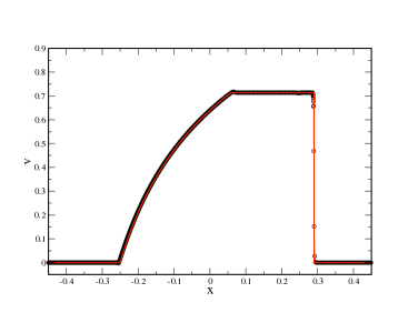
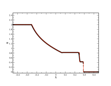
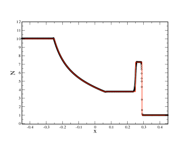
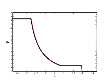
Figure 1: Results of the relativistic shock tube of test 1 at $t=0.35$: SPH results (circles) vs. exact solution (red line). From left to right, top to bottom: velocity (in units of $c$), specific energy, computing frame baryon number density and pressure.

As shown in Fig. 1, the numerical solution at $t=0.35$ (circles) agrees nearly perfectly with the exact one. Note in particular the absence of any spikes in $u$ and $P$ at the contact discontinuity (near $x\approx 0.25$), such spikes had plagued many earlier relativistic SPH formulations Rosswog:laguna93a ; Rosswog:siegler00a . The only places where we see possibly room for improvement is the contact discontinuity which is slightly smeared out and the slight over-/undershoots at the edges of the rarefaction fan.
In order to monitor how the error in the numerical solution decreases as a function of increased resolution, we calculate

$$L_{1}\equiv\frac{1}{N_{\rm part}}\sum_{b}^{N_{\rm part}}|v_{b}-v_{\rm ex}(r_{b})|,$$ (21)

where $N_{\rm part}$ is the number of SPH-particles, $v_{b}$ the (1D) velocity of SPH-particle $b$ and $v_{\rm ex}(r_{b})$ the exact solution for the velocity at position $r_{b}$. The results for $L_{1}$ are displayed in Fig. 2. The error $L_{1}$ decreases close to $\propto N_{\rm part}^{-1}$ (actually, the best fit is $L_{1}\propto N_{\rm part}^{-0.96}$), which is what is also found for Eulerian methods in tests that involve shocks. Therefore, for problems that involve shocks we consider the method first-order accurate.

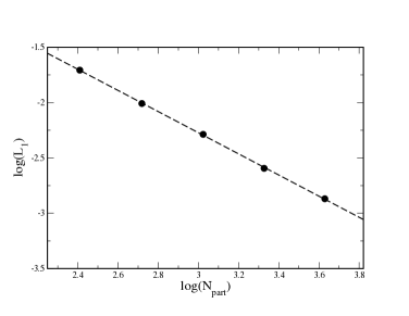
Figure 2: Decrease of the error as defined in Eq. (21) as a function of particle number for the relativistic shock tested in Riemann problem 1. The error decreases close to $L_{1}\propto N_{\rm part}^{-1}$.

The order of the method for smooth flows will be determined in the context of test 6.

4.2 Test 2: Riemann problem 2

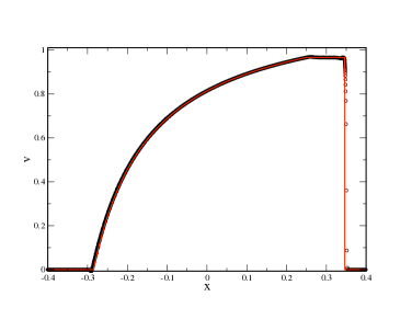
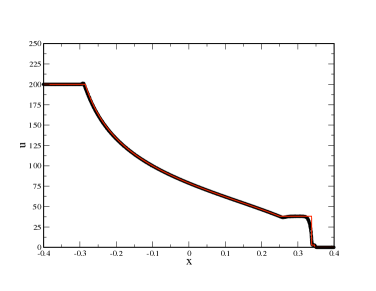
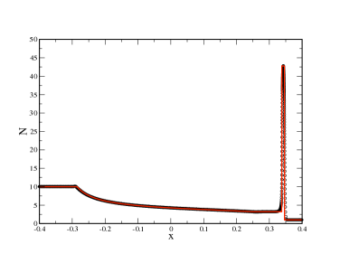
Figure 3: Same as previous test, but the initial left hand side pressure has been increased by a factor of 100. SPH results (at $t=0.35$) are shown as circles, the exact solution as red line. From left to right, top to bottom: velocity (in units of $c$), specific energy, computing frame baryon number density and pressure.

This test is a more violent version of test 1 in which we increase the initial left side pressure by a factor of 100, but leave the other properties, in particular the right-hand state, unchanged: $[P,\rho,v]_{\rm L}=[4000/3,10,0]$ and $[P,\rho,v]_{\rm R}=[10^{-6},1,0]$. This represents a challenging test since the post-shock density is compressed into a very narrow “spike”, at $t=0.35$ near $x\approx 0.35$. A maximum Lorentz-factor of $\gamma_{\rm max}\approx 3.85$ is reached in this test.
In Fig. 3 we show the SPH results (circles) of velocity $v$, specific energy $u$, the computing frame number density $N$ and the pressure $P$ at $t=0.35$ together with the exact solution of the problem (red line). Again the numerical solution is in excellent agreement with the exact one, only in the specific energy near the contact discontinuity occurs some smearing.

4.3 Test 3: Riemann problem 3

This test is an even more violent version of the previous tests. We now increase the initial left side pressure by a factor of 1000 with respect to test 1, but leave the other properties unchanged: $[P,\rho,v]_{\rm L}=[40000/3,10,0]$ and $[P,\rho,v]_{\rm R}=[10^{-6},1,0]$. The post-shock density is now compressed into a very narrow “needle” with a width of only $\approx 0.002$, the maximum Lorentz factor is 6.65.

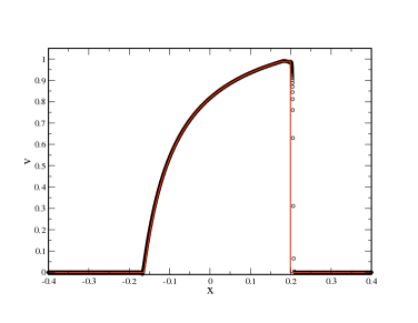
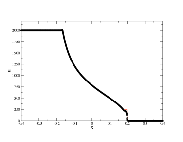
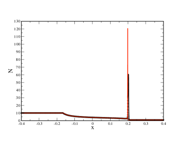
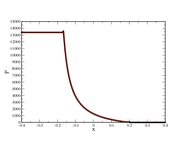
Figure 4: Same as first shock tube test, but the initial left hand side pressure has been increased by a factor of 1000. SPH results (at $t=0.2$) are shown as circles, the exact solution as red line. From left to right, top to bottom: velocity (in units of $c$), specific energy, computing frame baryon number density and pressure.

Fig. 4 shows the SPH results (circles) of velocity $v$, specific energy $u$, the computing frame number density $N$ and the pressure $P$ at $t=0.2$ together with the exact solution (red line). The overall performance in this extremely challenging test is still very good. The peak velocity plateau with $v\approx 0.99$ (panel 1) is very well captured, practically no oscillations behind the shock are visible. Of course, the “needle-like” appearance of the compressed density shell (panel 3) poses a serious problem to every numerical scheme at finite resolution. At the applied resolution, the numerical peak value of $N$ is only about half of the exact solution. Moreover, this extremely demanding test reveals an artifact of our scheme: the shock front is propagating at slightly too large a speed. This problem decreases with increasing numerical resolution and experimenting with the parameter $K$ of Eqs. (14) and (15) shows that it is related to the form of artificial viscosity, smaller offsets occur for lower values of the viscosity parameter $K$. Here further improvements would be desirable.

4.4 Test 4: Sinusoidally perturbed Riemann problem

This is a more extreme version of the test suggested by Rosswog:dolezal95 . It starts from an initial setup similar to a normal Riemann problem, but with the right state being sinusoidally perturbed. What makes this test challenging is that the smooth structure (sine wave) needs to be transported across the shock, i.e. kinetic energy needs to be dissipated into heat to avoid spurious post-shock oscillations, but not too much since otherwise the (physical!) sine oscillations in the post-shock state are not accurately captured. We use a polytropic exponent of $\Gamma=5/3$ and

$$[P,N,v]^{\rm L}=[1000,5,0]\quad{\rm and}\quad[P,N,v]^{\rm R}=[5,2+0.3\sin(50x),0].$$ (22)

as initial conditions, i.e. we have increased the initial left pressure by a factor of 200 in comparison to Rosswog:dolezal95 .

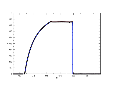
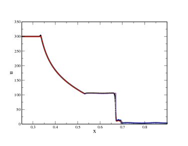
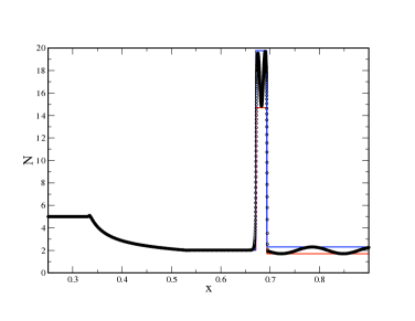
Figure 5: Riemann problem where the right-hand side is periodically perturbed. The SPH solution is shown as circles, the exact solution for Riemann problems with constant RHS densities $N_{\rm R}=2.3$ (blue) and $N_{\rm R}=1.7$ (red) are overlaid as solid lines.

The numerical result (circles) is shown in Fig. 5 together with two exact solutions, for the right-hand side densities $N_{\rm R}=2.3$ (solid blue) and $N_{\rm R}=1.7$ (solid red). All the transitions are located at the correct positions, in the post-shock density shell the solution nicely oscillates between the extremes indicated by the solid lines.

4.5 Test 5: Relativistic Einfeldt rarefaction test

The initial conditions of the Einfeldt rarefaction test Rosswog:einfeldt91 do not exhibit discontinuities in density or pressure, but the two halfs of the computational domain move in opposite directions and thereby create a very low-density region around the initial velocity discontinuity. This low-density region poses a serious challenge for some iterative Riemann solvers, which can return negative density/pressure values in this region. Here we generalize the test to a relativistic problem in which left/right states move with velocity -0.9/+0.9 away from the central position. For the left and right state we use $[P,n,v]_{\rm L}=[1,1,-0.9]$ and $[P,n,v]_{\rm R}=[1,1,0.9]$ and an adiabatic exponent of $\Gamma=4/3$. Note that here we have specified the local rest frame density, $n$, which is related to the computing frame density by Eq. (3). The SPH solution at $t=0.2$ is shown in Fig. 6 as circles, the exact solution is indicated by the solid red line. Small oscillations are visible near the center, mainly in $v$ and $u$, and over-/undershoots occur near the edges of the rarefaction fan, but overall the numerical solution is very close to the analytical one. In its current form, the code can stably handle velocities up to 0.99999, i.e. Lorentz factors $\gamma>200$, but at late times there are practically no more particles in the center (SPH’s approximation to the emerging near-vacuum), so that it becomes increasingly difficult to resolve the central velocity plateau.

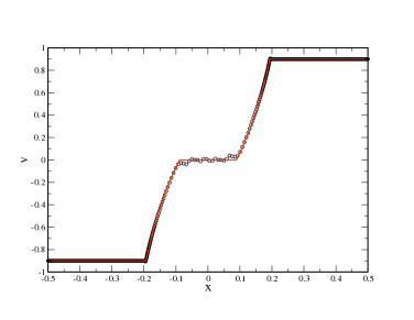
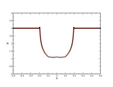
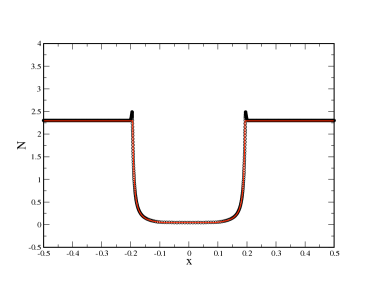
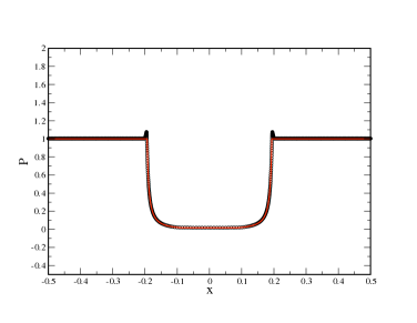
Figure 6: Relativistic version of the Einfeldt rarefaction test. Initially the flow has constant values of $n=1,P=1$ everywhere, $v_{L}=-0.9$ and $v_{R}=0.9$.

4.6 Test 6: Ultra-relativistic advection

In this test problem we explore the ability to accurately advect a smooth density pattern at an ultra-relativistic velocity across a periodic box. Since this test does not involve shocks we do not apply any artificial dissipation. We use only 500 equidistantly placed particles in the interval $[0,1]$, enforce periodic boundary conditions and use a polytropic exponent of $\Gamma=4/3$. We impose a computing frame number density $N(x)=N_{0}+\frac{1}{2}\sin(2\pi x)+\frac{1}{4}\sin(4\pi x)$, a constant velocity as large as $v=0.99999999$, corresponding to a Lorentz factor of $\gamma\approx 7071$, and instantiate a constant pressure corresponding to $P_{0}=(\Gamma-1)n_{0}u_{0}$, where $n_{0}=N_{0}/\gamma$ and $N_{0}=1$ and $u_{0}=1$. The specific energies are chosen so that each particle has the same pressure $P_{0}$. With these initial conditions the specified density pattern should just be advected across the box without being changed in shape.

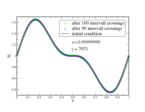
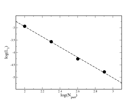
Figure 7: Left: Ultra-relativistic advection ($v=0.99999999$, Lorentz factor $\gamma=7071$) of a density pattern across a periodic box. The advection is essentially perfect, the patterns after 50 (blue circles) and 100 (green triangles) times crossing the box are virtually identical to the initial condition (red line). Right: Decrease of the $L_{1}$ error as a function of resolution, for smooth flows the method is second-order accurate.

The numerical result after 50 times (blue circles) and 100 times (green triangles) crossing the interval is displayed in Fig. 7, left panel. The advection is essentially perfect, no deviation from the initial condition (solid, red line) is visible.
We use this test to measure the convergence of the method in the case of smooth flow (for the case involving shocks, see the discussion at the end of test 1). Since for this test the velocity is constant everywhere, we use the computing frame number density $N$ to calculate $L_{1}$ similar to Eq. (21). We find that the error decreases very close to $L_{1}\propto N^{-2}$, see Fig. 7, right panel, which is the behavior that is theoretically expected for smooth functions, the used kernel and perfectly distributed particles Rosswog:monaghan92 (actually, we find as a best-fit exponent -2.07). Therefore, we consider the method second-order accurate for smooth flows.

5 Conclusions

We have summarized a new special-relativistic SPH formulation that is derived from the Lagrangian of an ideal fluid Rosswog:rosswog09d . As numerical variables it uses the canonical energy and momentum per baryon whose evolution equations follow stringently from the Euler-Lagrange equations. We have further applied the special-relativistic generalizations of the so-called “grad-h-terms” and a refined artificial viscosity scheme with time dependent parameters.
The main focus of this paper is the presentation of a set of challenging benchmark tests that complement those of the original paper Rosswog:rosswog09d . They show the excellent advection properties of the method, but also its ability to accurately handle even very strong relativistic shocks. In the extreme shock tube test 3, where the post-shock density shell is compressed into a width of only 0.1 % of the computational domain, we find the shock front to propagate at slightly too large a pace. This artifact ceases with increasing numerical resolution, but future improvements of this point would be desirable. We have further determined the convergence rate of the method in numerical experiments and find it first-order accurate when shocks are involved and second-order accurate for smooth flows.

Acknowledgment
This work was supported by the German Research Foundation under grant number 50245 DFG-RO-5.

References

- (1) S. Ayal, T. Piran, R. Oechslin, M. B. Davies, and S. Rosswog, Post-Newtonian Smoothed Particle Hydrodynamics, ApJ 550 (2001), 846–859.
- (2) T. W. Baumgarte and S. L. Shapiro, Numerical Relativity and Compact Binaries, Phys. Rep. 376 (2003), 41–131.
- (3) A. Bauswein, R. Oechslin, and H. -J. Janka, Discriminating Strange Star Mergers from Neutron Star Mergers by Gravitational-Wave Measurements, ArXiv e-prints (2009).
- (4) J. E. Chow and J.J. Monaghan, Ultrarelativistic SPH, J. Computat. Phys. 134 (1997), 296.
- (5) L. Del Zanna and N. Bucciantini, An Efficient Shock-capturing Central-type Scheme for Multidimensional Relativistic Flows. I. Hydrodynamics, A&A 390 (2002), 1177–1186.
- (6) A. Dolezal and S. S. M. Wong, Relativistic Hydrodynamics and Essentially Non-oscillatory Shock Capturing Schemes, J. Comp. Phys. 120 (1995), 266.
- (7) B. Einfeldt, P. L. Roe, C. D. Munz, and B. Sjogreen, On Godunov-type Methods Near Low Densities, J. Comput. Phys. 92 (1991), 273–295.
- (8) J. A. Faber, T. W. Baumgarte, S. L. Shapiro, K. Taniguchi, and F. A. Rasio, Dynamical Evolution of Black Hole-Neutron Star Binaries in General Relativity: Simulations of Tidal Disruption, Phys. Rev. D 73 (2006), no. 2, 024012.
- (9) J. A. Faber, P. Grandclément, and F. A. Rasio, Mergers of Irrotational Neutron Star Binaries in Conformally Flat Gravity, Phys. Rev. D 69 (2004), no. 12, 124036.
- (10) J. A. Faber and F. A. Rasio, Post-Newtonian SPH Calculations of Binary Neutron Star Coalescence: Method and First Results, Phys. Rev. D 62 (2000), no. 6, 064012.
- (11) J. A. Faber and F. A. Rasio, Post-Newtonian SPH Calculations of Binary Neutron Ntar Coalescence. III. Irrotational Systems and Gravitational Wave Spectra, Phys. Rev. D 65 (2002), no. 8, 084042.
- (12) J. A. Faber, F. A. Rasio, and J. B. Manor, Post-Newtonian Smoothed Particle Hydrodynamics Calculations of Binary Neutron Star Coalescence. II. Binary Mass Ratio, Equation of State, and Spin Dependence, Phys. Rev. D 63 (2001), no. 4, 044012.
- (13) V. Fock, Theory of Space, Time and Gravitation, Pergamon, Oxford, 1964.
- (14) J. Font, Numerical Hydrodynamics in General Relativity, Living Rev. Relativ. 3 (2000), 2.
- (15) J. F. Hawley, L. L. Smarr, and J. R. Wilson, A Numerical Study of Nonspherical Black Hole Accretion. II - Finite Differencing and Code Calibration, ApJS 55 (1984), 211–246.
- (16) A. Kheyfets, W. A. Miller, and W. H. Zurek, Covariant Smoothed Particle Hydrodynamics on a Curved Background, Phys. Rev. D 41 (1990), 451–454.
- (17) P. Laguna, W. A. Miller, and W. H. Zurek, Smoothed Particle Hydrodynamics Near a Black Hole, ApJ 404 (1993), 678–685.
- (18) P.J. Mann, A Relativistic Smoothed Particle Hydrodynamics Method Tested with the Shock Tube, Comp. Phys. Commun. (1991).
- (19) P.J. Mann, Smoothed Particle Hydrodynamics Applied to Relativistic Spherical Collapse, J. Comput. Phys. 107 (1993), 188–198.
- (20) J. M. Marti and E. Müller, Numerical Hydrodynamics in Special Relativity, Living Rev. Relativ. 6 (2003), 7.
- (21) J.M. Marti and E. Müller, Extension of the Piecewise Parabolic Method to One-Dimensional Relativistic Hydrodynamics, J. Comp. Phys. 123 (1996), 1.
- (22) J. J. Monaghan, Smoothed Particle Hydrodynamics, Ann. Rev. Astron. Astrophys. 30 (1992), 543.
- (23) J. J. Monaghan, SPH Compressible Turbulence, MNRAS 335 (2002), 843–852.
- (24) J. J. Monaghan, Smoothed Particle Hydrodynamics, Rep. Prog. Phys. 68 (2005), 1703–1759.
- (25) J. J. Monaghan and D. J. Price, Variational Principles for Relativistic Smoothed Particle Hydrodynamics, MNRAS 328 (2001), 381–392.
- (26) R. Oechslin, S. Rosswog, and F.-K. Thielemann, Conformally Flat Smoothed Particle Hydrodynamics Application to Neutron Star Mergers, Phys. Rev. D 65 (2002), no. 10, 103005.
- (27) S. Rosswog, Astrophysical Smooth Particle Hydrodynamics, New Astron. Rev. 53 (2009), 78.
- (28) S. Rosswog, Conservative, Special-relativistic Smooth Particle Hydrodynamics, submitted to J. Comp. Phys. (2009), eprint arXiv:0907.4890.
- (29) S. Rosswog, Relativistic Smooth Particle Hydrodynamics on a Given Background Space-time, Class. Quantum Grav. 27 (2010) 114108.
- (30) S. Siegler, Entwicklung und Untersuchung eines Smoothed Particle Hydrodynamics Verfahrens für relativistische Strömungen, Ph.D. thesis, Eberhard-Karls-Universität Tübingen, 2000.
- (31) S. Siegler and H. Riffert, Smoothed Particle Hydrodynamics Simulations of Ultrarelativistic Shocks with Artificial Viscosity, ApJ 531 (2000), 1053–1066.
- (32) V. Springel and L. Hernquist, Cosmological Smoothed Particle Hydrodynamics Simulations: the Entropy Equation, MNRAS 333 (2002), 649–664.