Space-and Time-like Electromagnetic Kaon Form Factors

Abstract

A simultaneous investigation of the space- and time-like electromagnetic form factors of the charged kaon is presented within the framework of light-cone QCD, with perturbative $k_{T}$-factorization including Sudakov suppression. The effects of power suppressed sub-leading twists and the genuine “soft” QCD corrections turn out to be dominant at low- and moderate-energies/momentum transfers $Q^{2}$. Our predictions agree well with the available moderate-energy experimental data, including the recent results from the CLEO measurements and certain estimates based on the phenomenological analyses of $J/\psi$ decays.

I Introduction

Electromagnetic form factors are interesting physical observables in hadronic physics which directly provide insights into the hadronic constituents, charge distributions, currents, color and flavor within the hadrons. Their precise knowledge is of fundamental importance for a realistic and accurate description of exclusive nuclear reactions that serve as ideal testing grounds for understanding the dynamics of confinement in QCD that have been grappling with physicists ever since the discovery of asymptotic freedom.

In the last few decades, there has been significant experimental efforts in extracting hadronic form factors (e.g., see. pion_exp ; ee-hh ; CLEO for the charged pion form factors ) from various exclusive processes. However, in case of the charged kaon form factors their behavior were very severely constrained due to absence of reliable experimental data. Since the mid-90s kaon photo-/electro-production experiments on reactions such as $A(\gamma,K)YB$ and $A(e,e^{\prime}K)YB$ (target $A$, produced hyperon $Y$ and recoil $B$) have invited some renewed interest in the study of kaon form factors, although the existing data is still too limited, restricted only to the very low space-like region, as low as $-q^{2}\leq 0.2$ GeV² kaon_exp_space . In the time-like region, there are more scattered data up to several GeV² (albeit with very large error-bars) for time-like processes such as $\gamma^{*}\rightarrow K^{+}K^{-}$, extracted from annihilation reactions such $J/\psi\rightarrow e^{+}e^{-}\rightarrow h^{+}h^{-}$ $(h=\pi,K,...)$ by applying suitable experimental cuts. A compilation of previously extracted kaon form factors for $q^{2}=Q^{2}<10$ GeV² is given in ee-hh . Recently, high precision measurements by the CLEO collaboration with first ever identified time-like kaons for $Q^{2}>4$ GeV² have yielded the following results: $\left|G_{K}(13.48\,{\rm GeV}^{2})\right|=0.063\pm 0.004$(stat)$\pm 0.001$(syst) and $Q^{2}\left|G_{K}(13.48\,{\rm GeV}^{2})\right|=0.85\pm 0.05$(stat) $\pm 0.02$(syst) GeV² CLEO . Note that in this paper, we shall use the symbol $G_{K}$ for the time-like kaon form factor to distinguish it from the space-like counterpart $F_{K}$.

Notwithstanding the aforementioned problem of paucity of quality statistics of the existing kaon data, the purpose of the paper is an effort to make a prediction for the charged kaon form factors using the framework of perturbative factorization Brodsky ; Radyushkin . In this way, we hope to throw some light on their possible behavior, especially, at the phenomenological intermediate energy region, where significant non-perturbative effects tend to spoil the asymptotic perturbative QCD (pQCD) results like the celebrated quark counting rule that predicts the scaling behavior $\{F,G\}_{K}(Q^{2})\sim 1/Q^{2}$ Brodsky ; FJ . Analyses of the pion form factors convincingly show that the standard pQCD with only twist-2 effects are much too small to explain the currently available experimental data at low- and moderate-energies. This calls for the inclusion of non-perturbative corrections from the genuine “soft” QCD Nest ; Isgur ; Stefanis1 ; Stefanis2 ; Bakulev and the sub-leading twists that can give rise to unnaturally large contributions at moderate range of $Q^{2}$-values. in particular, twist-3 enhancements were seen to be quite large in the previous studies for the space-like pion form factor GT ; Pasu ; Wei ; Huang ; Raha1 , the space-like kaon form factor Raha1 ; Wu , and in the studies of $B\rightarrow\pi$ transition form factors Keum ; Sanda ; Li ; Lu . In fact, the analysis presented in Raha2 shows a possible scenario where the contributions from the twist-3 terms in the time-like region can turn out to be exceptionally large. This seemed to resolve the bulk of the existing experimental discrepancy between the space- and the time-like pion data.

In this paper, following Raha1 ; Raha2 we extend the analysis to the space- and the time-like kaon form factors, where in addition to the twist-2 and twist-3 terms we explicitely include twist-4 corrections. Thereby, we show that the large twist-3 contributions are indeed a non-trivial aspect of our result in comparison with the other twist contributions, e.g., the 2-particle twist-4 contributions are explicitly shown to be about a third of the magnitude of the twist-2 terms. The paper is organized as follows: the second section briefly reviews the theoretical background, the third section deals with the details of our numerical analysis, results and discussions of the essential features of our results, and finally, we give our conclusions. For the purpose of book keeping, we provide a collection of relevant mathematical formulas in the appendix.

II Hard and Soft Kaon Form Factors

II.1 Factorized pQCD

The basic definitions of the space- and time-like electromagnetic form factors are given in terms of the following local matrix elements of the electromagnetic quark currents $J^{\rm em}_{\mu}$:

$$e(P^{\prime}+P)_{\mu}\,F_{K}(Q^{2})\!\! = \!\!\langle K^{\pm}(P^{\prime})|J^{\rm em}_{\mu}(0)|K^{\pm}(P)\rangle\,;$$

$$e(P^{\prime}-P)_{\mu}\,G_{K}(Q^{2})\!\! = \!\!\langle K^{+}(P^{\prime})\,K^{-}(P)|J^{\rm em}_{\mu}(0)|0\rangle\,;$$

$$J^{\rm em}_{\mu}\!\! = \!\!\sum^{\,}_{f}e_{f}\bar{q}_{f}\gamma_{\mu}q_{f}\,,$$ (1)

where $e$ is the electronic charge and $f$ is the flavor of the valence quark $q_{f}$ with charge $e_{f}$. In terms of light-cone co-ordinates, $P=(Q/\sqrt{2},0,{\mathbf{0}}_{T})$ and $P^{\prime}=(0,Q/\sqrt{2},{\mathbf{0}}_{T})$ are the incoming and outgoing external kaon momenta in the Breit-frame. In the space-like domain, $q^{2}=(P^{\prime}-P)^{2}=-Q^{2}\leq 0$, whereas for the time-like domain $q^{2}=(P^{\prime}+P)^{2}=Q^{2}\geq 0$. Here, $Q$ is assumed to be much larger compared to the kaon mass $m_{K}$, so that $P$ and $P^{\prime}$ almost lie along the light-cone directions.

In our approach, the total contributions to the charged kaon form factors come from the factorizable ”hard” parts $\{F,G\}^{\rm hard}_{K}(Q^{2})$ calculable within a perturbative framework, and the non-factorizable soft parts $\{F,G\}^{\rm soft}_{K}(Q^{2})$ relying on some non-perturbative techniques. The calculation of the hard parts rest on the essential assumption that at suitable high energy scales, the form factors are factorizable, i.e., separable into parts dominated by short- and long-distance dynamics. The short-distance dynamics are represented by the kernel of interactions between highly off-shell partons, above the so-called factorization scale $\mu_{F}$. While, the long-distance dynamics below the factorization scale are implicitly encoded within the kaonic wavefunctions/distribution amplitudes (DAs) with near-on-shell partons. Note that due to the well-known impulse or frozen approximation applicable for all high-energy exclusive mechanisms, the dominant contributions come entirely from the leading order (LO) Fock state, i.e., a $q\bar{q}$ valence quark configuration. The higher Fock states are neglected with contributions relatively suppressed by higher powers of $1/Q^{2}$. Fig. 1 shows two representative Feynman diagrams (there are 4 diagrams each for the space-and time-like cases) with LO hard kernels each having a single hard gluon exchange. These are convoluted with the incoming and outgoing kaon DAs to obtain the hard factorized kaon form factors. In this analysis, we calculate $\{F,G\}^{\rm hard}_{K}(Q^{2})$ up to twist-4 accuracy in the two-particle sector, including explicit transverse momentum ($k_{T}$) dependence (TMD) of the constituent valence partons. The non-factorizable soft contributions, on the other hand, can either be calculated using Drell-Yan-West type of wavefunctions overlap ansatz DYW , or from QCD sum rules (QCDSR) incorporating local quark-hadron duality (LD) principle Nest . Both these approaches to parameterize the genuine soft contributions are known to give very similar results. In this work, we follow the latter approach. The above assertion can then be summarized by

$$\{F,G\}_{K}(Q^{2})\!\! = \!\!\{F,G\}^{\rm soft}_{K}(Q^{2})+\{F,G\}^{\rm hard}_{K}(Q^{2})\,;$$

$$\{F,G\}^{\rm hard}_{K}(Q^{2})\!\! = \!\!\Delta\{F,G\}^{\rm twist2}_{K}(Q^{2})+\Delta\{F,G\}^{\rm twist3}_{K}(Q^{2})+\Delta\{F,G\}^{\rm twist4}_{K}(Q^{2})\,.$$ (2)

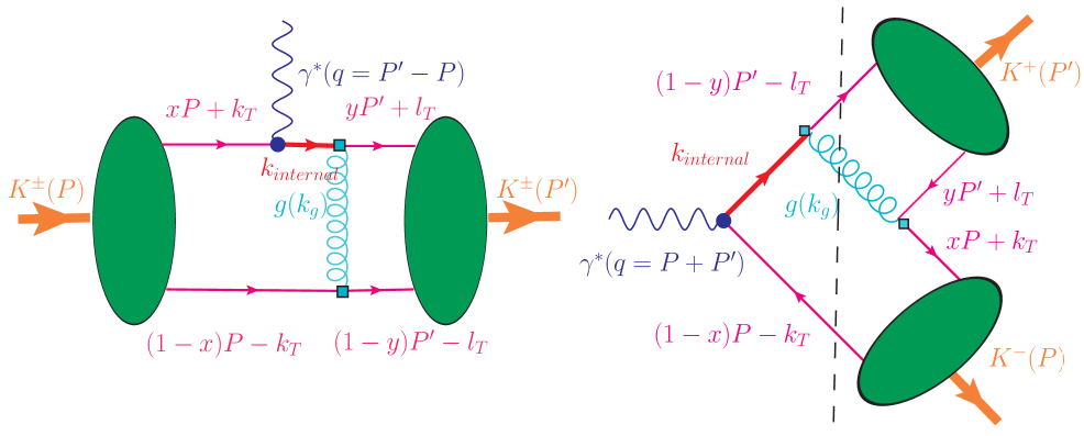
Figure 1: LO Feynman diagrams in pQCD for hard contributions to the charged kaon form factors in the space-like (left) and the time-like (right) region.

The principal inputs for determining the factorized kaon form factors are the collinear/light-cone DAs which encode all the non-perturbative physics. They are universal in nature (frame or process independent), in a sense, once they are determined at a certain process, they could yield predictions for another. To next-to-leading order (NLO) in conformal twist expansion there are one 2-particle twist-2 DA $\phi_{2;K}$ with an axial-vector structure, two 2-particle twist-3 DAs - $\phi^{p}_{3;K}$ with a pseudo-scalar structure and $\phi^{\sigma}_{3;K}$ with a pseudo-tensor structure, and finally, two 2-particle twist-4 DAs ${\mathbb{A}}_{4;K}$ and ${\mathbb{B}}_{4;K}=g_{4;K}-\phi_{2;K}$ both having pseudo-scalar structures Filyanov ; Ball ; Lenz . As an example for $K^{-}$, we display the twist-2 DA in terms of the following pseudo-scalar matrix element with $\xi=2x-1$:

$$\langle 0\left|\bar{u}(z)\,\gamma_{\mu}\gamma_{5}\,s(-z)\right|K^{-}(P)\rangle=iP_{\mu}\,\int^{1}_{0}dx\,e^{i\xi(Pz)}\,\phi_{2;K}(x,\mu^{2})\,,$$ (3)

with the normalization condition

$$N_{2;K}=\int^{1}_{0}\,\phi_{2;K}(x,\mu^{2})\,dx=\frac{f_{K}}{2\sqrt{2N_{c}}}\,,$$ (4)

where $f_{K}$ is the kaon decay constant defined in the local limit $z\rightarrow 0$ by

$$\left<0\left|\bar{u}(0)\,\gamma_{\mu}\gamma_{5}\,s(0)\right|K^{-}(P)\right>=if_{K}P_{\mu}\,.$$ (5)

In the above equations, $x$ is the collinear/light-cone momentum fraction ($x_{i}=k^{+}/P^{+}$) carried by the individual valence quarks ($x$ for the $s$ quark and $\bar{x}=1-x$ for the anti-quark $\bar{u}$.) Note that the gauge-connection factor in the above matrix element is assumed implicitly. To the leading logarithmic accuracy $\phi_{2;K}$ satisfies the well-known ER-BL evolution equation Brodsky ; Radyushkin and can be expressed as an irreducible representation of the special collinear conformal group S${\mathbb{L}}(2,{\mathbb{R}})$, in terms of standard Gagenbauer Polynomials $C^{3/2}_{n}(\xi)$:

$$\phi_{2;K}(x,\mu^{2})=\phi^{(\rm as)}_{2;K}(x)\,\sum^{\infty}_{n=0}a^{K}_{n}(\mu^{2}_{0})\,C^{3/2}_{n}(\xi)\left(\frac{\alpha_{s}(\mu^{2})}{\alpha_{s}(\mu^{2}_{0})}\right)^{-4\gamma^{(0)}_{n}/9}+{\mathcal{O}}(\alpha_{s})\,,$$ (6)

with the asymptotic twist-2 DA given by

$$\phi^{(\rm as)}_{2;K}(x)=\phi_{2;K}(x,\mu^{2}\rightarrow\infty)=\frac{3f_{K}}{\sqrt{2N_{c}}}\,x(1-x)\,.$$ (7)

The standard QCD $\overline{\rm{MS}}$ running coupling $\alpha_{s}(\mu^{2})$ to two-loop accuracy is given by

$$\frac{\alpha_{s}(\mu^{2})}{\pi}=\frac{1}{\beta_{0}\ln(\mu^{2}/\Lambda^{2}_{\rm QCD})}-\frac{\beta_{1}\ln(\ln(\mu^{2}/\Lambda^{2}_{\rm QCD}))}{\beta^{3}_{0}\ln^{2}(\mu^{2}/\Lambda^{2}_{\rm QCD})}$$ (8)

with $\Lambda_{\rm QCD}\approx 0.2$ GeV, $\beta_{0}\!=(11N_{c}-2N_{f})/12=\!9/4$ and $\beta_{1}\!=(51N_{c}-19N_{f})/24=\!4$ for $N_{c}\!=\!N_{f}\!=\!3$. The ratio of the QCD couplings represents the renormalization group (RG) evolution of the Gagenbauer moments $a^{K}_{n}$ from the normalization scale $\mu_{0}\approx 1$ GeV to the generic scale $\mu$, with LO anomalous dimensions given by

$$\gamma^{(0)}_{n}=\frac{4}{3}\left\{\frac{1}{4}+\sum^{n+1}_{k=2}\frac{1}{k}-\frac{1}{2(n+1)(n+2)}\right\}\geq 0$$ (9)

The Gagenbauer moments represent the genuine non-perturbative inputs to the DAs and are usually determined using lattice simulations or from light-cone sum rules (LCSR). In this work, we use the latter inputs, since the moments for the higher twist DAs are yet to be determined precisely in Lattice QCD. Note that the lower order moments in both approaches are known to be in good agreement with each other. However, dealing with such an infinite number of terms in the non-asymptotic DAs become a matter of technical challenge as the higher order moments are extremely difficult to determine. Hence, for practical simplicity of calculation, one truncates the DA series up to the first couple of terms only. Moreover, the increasing anomalous dimensions tend to suppress the higher order terms. In this analysis, we consider the series up to the term with the second moment $a^{K}_{2}$. The rest of the non-asymptotic collinear DAs, i.e., the 2-particle twist-3 and twist-4 DAs which we also consider in this work, have more elaborate expressions and are, therefore, relegated to the appendix along with their RG evolutions. A summary of the relevant DA parameters determined from LCSR at the normalization scale of $\mu_{0}\approx 1$ GeV is presented in Table. 1.

A common feature of DAs derived from LCSR is that they are endpoint dominated due to large kinematic enhancements when the light-cone momentum fractions tend to the endpoints (i.e., $x\rightarrow 0,1$). One possible way to suppress such artificial enhancement is to use the Brodsky-Huang-Lepage (BLH) Gaussian parameterization BHL , where the intrinsic TMD of the valance partons within the full kaon wavefunction $\Psi_{t;K}$ (for each twist $t=2,3,4$) is explicitly modeled by including an addition wavefunction $\Sigma_{t;K}$, i.e.,

$$\Psi_{t;K}(x,{\mathbf{k}}_{T},\mu^{2},{\mathcal{M}}_{\{u,d,s\}})=A_{t;K}\,\phi_{t;K}(x,\mu^{2})\,\Sigma_{t;K}(x,{\mathbf{k}}_{T},{\mathcal{M}}_{\{u,d,s\}})\,,$$ (10)

where the form of $\Sigma_{t;K}$ is chosen similar to that of a harmonic oscillator wavefunction that can maximally suppress such endpoint effects and given by

$$\Sigma_{t;K}(x,{\mathbf{k}}_{T},{\mathcal{M}}_{\{u,d,s\}})=\frac{16\pi^{2}\beta_{t;K}^{2}}{x(1-x)}\,{\rm{exp}}\left[-\beta^{2}_{t;K}\left(\frac{{\mathcal{M}}^{2}_{s}+{\mathbf{k}}^{2}_{T}}{x}+\frac{{\mathcal{M}}^{2}_{u,d}+{\mathbf{k}}^{2}_{T}}{1-x}\right)\right]\,.$$ (11)

Note that the constituent quark masses ${\mathcal{M}}_{\{u,d,s\}}$ are introduced to parameterize the QCD vacuum effects, while the parameters $A_{t;K}$ and $\beta_{t;K}$ for the individual twists are phenomenologically extracted as described in the next section (also see, Raha1 ). Next to obtain the full TMD modified kaon DAs $\tilde{{\mathcal{P}}}_{t;K}$ in the impact parameter or $b$-representation, we use the Brodsky-Lepage definition of the DA Brodsky , yielding

$$\tilde{{\mathcal{P}}}_{t;K}(x,b,\mu^{2},{\mathcal{M}}_{\{u,d,s\}})\!\! = \!\!\int^{1/b^{2}}_{0}\frac{d^{2}{\mathbf{k}}_{T}}{16\pi^{3}}\,\Psi_{t;M}(x,{\mathbf{k}}_{T},\mu^{2},{\mathcal{M}}_{\{u,d,s\}})$$ (12)

$$= \!\!{A_{t;K}}\,\phi_{t;K}(x,\mu^{2})\,{\rm{exp}}\left[-{\beta^{2}_{t;K}}\left(\frac{{{\mathcal{M}}^{2}_{s}}}{x}+\frac{{{\mathcal{M}}^{2}_{u,d}}}{1-x}\right)\right]$$

$$\qquad\times{\rm{exp}}\left[-\frac{b^{2}x(1-x)}{4{\beta^{2}_{t;K}}}\right]\,.$$

In Figs. 2 and 3, we show the various collinear DAs (which are endpoint enhanced) and the modified BHL DAs (which are endpoint suppressed) respectively. We also display the corresponding asymptotic forms of the DAs.

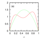
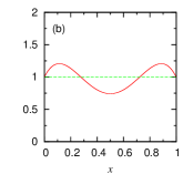
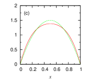
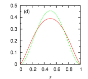
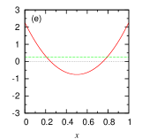
Figure 2: The collinear twist-2 and the 2-particle twist-3 and twist-4 DAs for the kaon (modulo, the normalizations $N_{t;K}$), shown using solid (red) lines, i.e., (a) $\phi_{2;K}(x,\mu_{0}^{2})$, (b) $\phi^{\,p}_{3;K}(x,\mu_{0}^{2})$, (c) $\phi^{\,\sigma}_{3;K}(x,\mu_{0}^{2})$, (d) $m^{2}_{K}{\mathbb{A}}_{4;K}(x,\mu_{0}^{2})$, and (e) $m^{2}_{K}g_{4;K}(x,\mu_{0}^{2})$, along with their respective asymptotic DAs, shown using dashed (green) lines. The DAs are defined at the scale $\mu_{0}=1$ GeV.

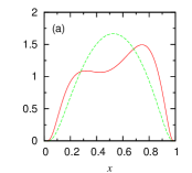
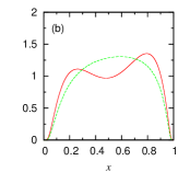
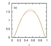
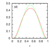
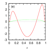
Figure 3: The BHL modified twist-2 and the 2-particle twist-3 and twist-4 DAs for the kaon (modulo, the normalizations $N_{t;K}$), shown using solid (red) lines, i.e., (a) $\tilde{\mathcal{P}}_{2;K}(x,\mu_{0}^{2})$, (b) $\tilde{\mathcal{P}}^{\,p}_{3;K}(x,\mu_{0}^{2})$, (c) $\tilde{\mathcal{P}}^{\,\sigma}_{3;K}(x,\mu_{0}^{2})$, (d) $m^{2}_{K}\tilde{\mathcal{P}}^{\mathbb{A}}_{4;K}(x,\mu_{0}^{2})$, and (e) $m^{2}_{K}\tilde{\mathcal{P}}^{g}_{4;K}(x,\mu_{0}^{2})$, along with their respective asymptotic DAs, shown using dashed (green) lines. The DAs are defined at the scale $\mu_{0}=1$ GeV.

The inclusion of the TMD in the hard scattering kernel at the same time also serves as a natural regulator for possible endpoint enhancements. However, this leads to the appearance of large logarithms in the kernel due to incomplete cancellation between soft gluon bremsstrahlung and radiative corrections that may spoil the perturbative convergence and, hence, the validity of the collinear factorization. While, the large single-logarithms such as $\alpha_{s}\ln Q^{2}$ can be effectively tackled using usual RG techniques like UV divergences, the large double-logarithms or Sudakov logarithms involving TMD such as $\alpha_{s}\ln^{2}(Q^{2}/k^{2}_{T})$, arising from the overlap of the leading soft and collinear kinematic regions of radiative gluons, can not be similarly handled in ordinary fixed order perturbation theory. The alternative is to use resummation techniques to all orders in the strong coupling constant $\alpha_{s}$ which organizes the double-logarithms within exponential Sudakov factors to get eventually systematically absorbed by a re-definition of the DAs. Such Sudakov factors represent the perturbative tail of the DAs and suppress non-perturbative enhancement that arise from constituent partonic configurations which involve large impact space separations. For a review of the Sudakov form factors and their application to exclusive physics, the reader is referred to Stefanis2 ; Lu ; Botts ; LiSterman . There may be other radiative collinear double-logarithms such as $\alpha_{s}\ln^{2}x$ which may be resummed using threshold resummation Sanda ; Li to suppress additional collinear enhancements in the kernel. The threshold resummation along with the Sudakov resummation arising from different subprocesses in pQCD factorization provides natural suppression to the endpoint and other non-perturbative enhancements and are relevant in the range of currently probed energy/momentum transfer values. The upshot is that the hard perturbative contributions are enhanced relative to the non-perturbative contributions improving convergence significantly and making pQCD evaluation of exclusive form factors self-consistent toward lower values of $Q^{2}$, where it may not be otherwise justified.

Such techniques of systematic organization of the potentially large logarithmic contributions is a modification from the standard collinear factorization and is generally termed as the ”$k_{T}$-factorization”, that has been widely applied to inclusive as well as exclusive processes kT . However, unlike the familiar collinear factorization theorem, the $k_{T}$-factorization is currently considered only at the level of a conjecture which is yet to be proven to all orders in perturbation theory (this is a highly debatable issue and, in fact, not yet fully recognized, e.g., see JPMa for a different viewpoint.) To demonstrate that $k_{T}$-factorization is indeed a systematic tool, demands higher order calculations which may be very challenging. However, in this paper, we shall implicitly assume the validity of such a modified factorization without proving it and restrict ourselves at the tree level analysis of the $k_{T}$-dependent hard kernel. Moreover, in LiNagashima , the $k_{T}$-factorization was proven at the level of twist-2 accuracy, while the collinear factorization was explicitely shown to be valid at the twist-3 accuracy in the case of the $\pi\gamma^{*}\rightarrow\gamma$ transition form factor. Our analysis is, therefore, based on the key assumption that the same formalism could be straightforwardly extended to the elastic kaon form factors.

At the leading order $\sim 1/Q^{2}$, the twist-2 and the two-particle twist-4 terms contribute to the hard kernels which have exactly the same expression given by

$$T^{\rm(t=2,4;LO)}_{\rm hard}(x,y,Q^{2},{\mathbf{k}}_{T},{\mathbf{l}}_{T},\mu^{2})=\frac{\pm 16\pi\,{\mathcal{C}}_{F}\,\alpha_{s}(\mu^{2})\,xQ^{2}}{(xQ^{2}\pm{\mathbf{k}}_{T}^{2})(xy\,Q^{2}\pm({\mathbf{k}}_{T}-{\mathbf{l}}_{T})^{2})}\,,$$ (13)

while, the ${\mathcal{O}}(1/Q^{4})$ power suppressed 2-particle twist-3 and twist-4 hard kernels are, respectively, given by

$$T^{\rm(t=3)}_{\rm hard}(x,y,Q^{2},{\mathbf{k}}_{T},{\mathbf{l}}_{T},\mu^{2})\!\! = \!\!\frac{32\pi\,{\mathcal{C}}_{F}\,\alpha_{s}(\mu^{2})\,x}{(xQ^{2}\pm{\mathbf{k}}_{T}^{2})(xy\,Q^{2}\pm({\mathbf{k}}_{T}-{\mathbf{l}}_{T})^{2})}\,;$$

$$T^{\rm(t=4;NLO)}_{\rm hard}(x,y,Q^{2},{\mathbf{k}}_{T},{\mathbf{l}}_{T},\mu^{2})\!\! = \!\!\frac{48\pi\,{\mathcal{C}}_{F}\,\alpha_{s}(\mu^{2})}{(xQ^{2}\pm{\mathbf{k}}_{T}^{2})(xy\,Q^{2}\pm({\mathbf{k}}_{T}-{\mathbf{l}}_{T})^{2})}\,.$$ (14)

In the above expressions, ${\mathcal{C}}_{F}=4/3$, the ”$+$” signs correspond to the space-like case and the ”$-$” signs correspond to the time-like case; ${\mathbf{k}}_{T}$ and ${\mathbf{l}}_{T}$ are, respectively, the initial and final relative transverse momenta of the valence quarks, and $x$ and $y$ are the corresponding light-cone momentum fractions. Note that the factors in the denominators that arise from the parton propagators develop poles in the time-like region.

To obtain the hard form factors, we use the following momentum space projection operator for the DAs with the different twist structures:

$${\mathcal{M}}^{K}_{\alpha\beta}\! = \!\frac{i}{4}\left\{P\!\!\!\!/\gamma_{5}\left(\Psi_{2;K}-\frac{1}{4}m^{2}_{K}\Psi^{\mathbb{A}}_{4;K}\partial^{2}_{k_{T}}\right)+m^{2}_{K}\gamma_{5}\left(\frac{\bar{P}\!\!\!\!/}{\bar{P}\cdot P}\frac{\partial}{\partial x}\left(\int^{x}_{0}\Psi^{\mathbb{B}}_{4;K}\right)-\Psi^{\mathbb{A}}_{4;K}\partial_{k_{T}}\!\!\!\!\!\!\!\!/\,\,\,\,\right)\right.$$ (15)

$$\!\!-\left.\mu_{K}\gamma_{5}\left(\Psi^{p}_{3;K}-\frac{i}{6}\sigma_{\mu\nu}n^{\mu}\bar{n}^{\nu}\frac{\partial}{\partial x}\Psi^{\sigma}_{3;K}+\frac{i}{6}\sigma_{\mu\nu}P^{\mu}\,\Psi^{\sigma}_{3;K}\,\partial^{\,\nu}_{k_{T}}\right)\right\}_{\alpha\beta}\,;\,\bar{P}=|P|\bar{n}\,,$$

where $\mu_{K}=\frac{m^{2}_{K}}{m_{u}+m_{s}}$ GeV is the ”chiral-enhancement” parameter arising in the standard definition of the 2-particle twist-3 DAs (see, appendix), $\Psi^{\mathbb{B}}_{4;K}=\Psi^{g}_{4;K}-\Psi_{2;K}$, $\partial_{k_{T}}\!\!\!\!\!\!\!\!/\,\,\,\,\equiv\gamma^{\mu}\partial/\partial{k^{\mu}_{T}}$, $n=(1,0,{\mathbf{0}}_{T})$ the unit vector in the “$+$” direction, and $\bar{n}=(0,1,{\mathbf{0}}_{T})$ the unit vector in the “$-$” direction. Setting the renormalization/factorization scale to the magnitude of the incoming or outgoing kaon momentum i.e., $\mu=|P|=|P^{\prime}|=Q/\sqrt{2}$ and convolving the projection operators for the kaon DAs with the hard kernels using factorization formula (symbolically, ${\mathcal{M}}^{\dagger}_{\rm K;out}\otimes T^{\rm LO}_{\rm hard}\otimes{\mathcal{M}}_{\rm K;in}$), we have

$$\left(P^{\prime}\pm P\right)_{\mu}\!\!\! \!\!\!\!\!\!\{F,G\}^{\rm hard}_{K}(Q^{2})$$ (16)

$$= \!\!\int^{1}_{0}dxdy\int\frac{d^{2}{\mathbf{k}}_{T}}{16\pi^{3}}\,\frac{d^{2}{\mathbf{l}}_{T}}{16\pi^{3}}\,\left(\frac{4\pi\alpha_{s}(t)\,{\mathcal{C}}_{F}}{3}\right){\rm exp}\left[-i{\mathbf{k}}_{T}\cdot{\mathbf{b}}_{1}-i{\mathbf{l}}_{T}\cdot{\mathbf{b}}_{2}\right]$$

$${\mathbf{T}r}\!\left[\frac{\gamma^{\nu}{\mathcal{M}}_{K;out}^{\dagger}\,\gamma_{\nu}\,/\!\!\!k_{internal}\,\gamma_{\mu}\,{\mathcal{M}}_{K;in}}{(k^{2}_{internal}+i\epsilon)\,(k^{2}_{g}+i\epsilon)}+{\rm 3\,diagrams}\right]\,{\mathcal{U}}_{\rm RGE}(t,\mu)$$

$$\times\,S_{t}(x)\,{\rm exp}\left[-S(x,y,|{\mathbf{k}}_{T}|\sim 1/b_{1},|{\mathbf{l}}_{T}|\sim 1/b_{2},\mu)\right]\,,$$

where $k_{internal}$ and $k_{g}$ are the internal quark and gluon momenta, respectively, as shown in Fig.1. Also, in the above equation

$${\mathcal{U}}_{\rm RGE}(t,\mu)={\rm exp}\left[4\int^{\mu}_{t}\frac{d\bar{\mu}}{\bar{\mu}}\gamma_{q}(\alpha_{s}({\bar{\mu}}^{2}))\right]\,;\,\gamma_{q}(\alpha_{s}({\bar{\mu}}^{2}))=-\frac{\alpha_{s}({\bar{\mu}}^{2})}{\pi}\,,$$ (17)

represents the RG evolution factor for the scattering kernel from the “upper-factorization” scale $t={\rm max}(\sqrt{x}\,Q,1/b_{1},1/b_{2})$ to the renormalization scale $\mu=Q/\sqrt{2}$, and $\gamma_{q}$ is the quark anomalous dimension. The expression for the Sudakov exponent $S(x,y,b_{1},b_{2},Q)$ (after absorbing the RG factor from the kernel) is given by LiSterman

$$S(x,y,b_{1},b_{2},Q)\! = \!s(xQ,b_{1})+s((1-x)Q,b_{1})+s(yQ,b_{2})+s((1-y)Q,b_{2})$$ (18)

$$+2\int^{t}_{1/b_{1}}\frac{d\bar{\mu}}{\bar{\mu}}\gamma_{q}(\alpha_{s}({\bar{\mu}}^{2}))+2\int^{t}_{1/b_{2}}\frac{d\bar{\mu}}{\bar{\mu}}\gamma_{q}(\alpha_{s}({\bar{\mu}}^{2}))\,,$$

where

$$s(xQ,1/b)\equiv s(x\mu,1/b)=\int^{x\mu}_{1/b}\frac{d\bar{\mu}}{\bar{\mu}}\left[\ln\left(\frac{\mu}{\bar{\mu}}\right){\mathcal{A}}(\alpha_{s}(\bar{\mu}^{2}))+{\mathcal{B}}(\alpha_{s}(\bar{\mu}^{2}))\right]\,,$$ (19)

where the “lower-factorization” scales $1/b_{1}$, $1/b_{2}>\Lambda_{\rm QCD}$ serve to separate the perturbative from the non-perturbative transverse distances which are also typically the scales that provide a natural starting point of the evolution of the kaon wavefunctions. In the above equations, the so-called “cusp” anomalous dimensions ${\mathcal{A}}$ and ${\mathcal{B}}$, to one-loop accuracy are given by

$${\mathcal{A}}(\alpha_{s}(\mu^{2}))\! = \!{\mathcal{C}}_{F}\frac{\alpha_{s}(\mu^{2})}{\pi}+\left[\left(\frac{67}{27}-\frac{\pi^{2}}{9}\right)N_{c}-\frac{10}{27}N_{f}+\frac{8}{3}\beta_{0}\ln\left(\frac{e^{\gamma_{E}}}{2}\right)\right]\left(\frac{\alpha_{s}(\mu^{2})}{\pi}\right)^{2}\,,$$

$${\mathcal{B}}(\alpha_{s}(\mu^{2}))\! = \!\frac{2}{3}\frac{\alpha_{s}(\mu^{2})}{\pi}\ln\left(\frac{e^{2\gamma_{E}-1}}{2}\right)\,.$$ (20)

The exact form of the threshold resummation “jet” function $S_{t}(x)$ in Eq. 16 involves a one parameter integration, but in practice it is more convenient to take the simple parameterization proposed in Sanda ; Li :

$$S_{t}(x)=\frac{2^{1+2c}\Gamma(3/2+c)}{\sqrt{\pi}\Gamma(1+c)}\left[x(1-x)\right]^{c}\,,$$ (21)

where the parameter $c\approx 0.3$ for light pseudo-scalar mesons like the pion and the kaon.

Now we present the factorized result for the hard kaon form factors up to twist-4 corrections as follows:

$$\{F,G\}^{\rm hard}_{K}(Q^{2})\!\! = \!\!\delta\{F,G\}^{\rm twist2}_{K}(Q^{2})+\delta\{F,G\}^{\rm twist3}_{K}(Q^{2})+\delta\{F,G\}^{\rm twist4}_{K}(Q^{2})\,;$$

$$\delta\{F,G\}^{\rm twist4}_{K}(Q^{2})\!\! = \!\!\delta\{F,G\}^{\rm twist4;LO}_{K}(Q^{2})+\delta\{F,G\}^{\rm twist4;NLO}_{K}(Q^{2})\,,$$ (22)

where the leading twist-2 and twist-4 corrections are expressed by the following integral representations in the impact parameter space:

$$\delta\{F,G\}^{\rm twist2}_{K}\!\! \!\!\!(Q^{2})+\delta\{F,G\}^{\rm twist4;LO}_{K}(Q^{2})=32\pi Q^{2}{\mathcal{C}}_{F}\int^{1}_{0}x\,dxdy\int^{\infty}_{0}b_{1}db_{1}b_{2}db_{2}\,\alpha_{s}(t)$$ (23)

$$\times\,\left[\pm\frac{1}{2}\,{\mathcal{P}}_{2;K}(x,b_{1})\,{\mathcal{P}}_{2;K}(y,b_{2})\mp\,m^{2}_{K}\,\frac{b^{2}_{2}}{8}\,{\mathcal{P}}_{2;K}(x,b_{1})\,{\mathcal{P}}^{\mathbb{A}}_{4;K}(y,b_{2})\right.$$

$$\left.\mp\,m^{2}_{K}\,\frac{b^{2}_{1}}{8}\,{\mathcal{P}}^{\mathbb{A}}_{4;K}(x,b_{1})\,{\mathcal{P}}_{2;K}(y,b_{2})+{\mathcal{O}}\left(m^{4}_{K}b^{4}_{1},m^{4}_{K}b^{4}_{2}\right)\right]$$

$$\times\,H_{\pm}(x,y,Q,b_{1},b_{2})\,{\rm exp}\left[-S(x,y,b_{1},b_{2},Q)\right]\,S_{t}(x)\,,$$

while, the power suppressed twist-3 and twist-4 corrections are given by

$$\delta\{F,G\}^{\rm twist3}_{K}\!\!\!\! \!\!(Q^{2})+\delta\{F,G\}^{\rm twist4;NLO}_{K}(Q^{2})=32\pi Q^{2}{\mathcal{C}}_{F}\int^{1}_{0}dxdy\int^{\infty}_{0}b_{1}db_{1}b_{2}db_{2}\,\alpha_{s}(t)$$ (24)

$$\times\,\left[\frac{\mu^{2}_{K}}{Q^{2}}\left({\bar{x}}\,{\mathcal{P}}^{\,p}_{3;K}(x,b_{1})\,{\mathcal{P}}^{\,p}_{3;K}(y,b_{2})+\frac{(1+x)}{6}\,\frac{\partial}{\partial x}{\mathcal{P}}^{\,\sigma}_{3;K}(x,b_{1})\,{\mathcal{P}}^{\,p}_{3;K}(y,b_{2})\right.\right.$$

$$\left.\left.+\,\frac{1}{2}{\mathcal{P}}^{\,\sigma}_{3;K}(x,b_{1})\,{\mathcal{P}}^{\,p}_{3;K}(y,b_{2})\right)+\frac{3m^{2}_{K}}{2Q^{2}}\left(\int^{x}_{0}d\zeta\,{\mathcal{P}}^{\mathbb{B}}_{4;K}(\zeta,b_{1})\right)\right.$$

$$\left.\times\,\left({\mathcal{P}}_{2;K}(y,b_{2})-\,m^{2}_{K}\,\frac{b^{2}_{2}}{4}\,{\mathcal{P}}^{\mathbb{A}}_{4;K}(y,b_{2})\right)+{\mathcal{O}}\left(m^{4}_{K}b^{4}_{1},m^{4}_{K}b^{4}_{2}\right)\right]$$

$$\times\,\,H_{\pm}(x,y,Q,b_{1},b_{2})\,{\rm exp}[-S(x,y,b_{1},b_{2},Q)]\,S_{t}(x)\,,$$

where ${\mathcal{P}}_{t;K}(x,b)\equiv\tilde{\mathcal{P}}_{t;K}(x,b,1/b^{2},{\mathcal{M}}_{\{u,d,s\}})$, and ${\mathcal{P}}^{\mathbb{B}}_{4;K}\!=\!{\mathcal{P}}^{g}_{4;K}-{\mathcal{P}}_{2;K}$. Note that the “LO” and “NLO” used in the above equation should not be confused with the usual terminologies associated with perturbative expansions in terms of $\alpha_{s}$ but rather in the sense of operator product expansion (OPE) terms. In the impact representation, the space- and time-like hard kernels (the part of the scattering kernel that is common to all the twists) could be expressed in terms of standard Bessel functions $K_{0},\,I_{0},\,J_{0}$ and $H^{(1)}_{0}$ and are given by

$$H_{+}(x,y,Q,b_{1},b_{2})\! = \!K_{0}(\sqrt{xy}\,Qb_{2})$$ (25)

$$\times\left[\theta(b_{1}-b_{2})K_{0}(\sqrt{x}\,Qb_{1})I_{0}(\sqrt{x}\,Qb_{2})\right.$$

$$+\left.\theta(b_{2}-b_{1})K_{0}(\sqrt{x}\,Qb_{2})I_{0}(\sqrt{x}\,Qb_{1})\right]\,;$$

$$H_{-}(x,y,Q,b_{1},b_{2})\!\! = \!\!\left(\frac{i\pi}{2}\right)^{2}H^{(1)}_{0}(\sqrt{xy}\,Qb_{2})$$ (26)

$$\times\left[\theta(b_{1}-b_{2})H^{(1)}_{0}(\sqrt{x}\,Qb_{1})J_{0}(\sqrt{x}\,Qb_{2})\right.$$

$$+\left.\theta(b_{2}-b_{1})H^{(1)}_{0}(\sqrt{x}\,Qb_{2})J_{0}(\sqrt{x}\,Qb_{1})\right]\,,$$

where $H_{+}$ is a real-valued function and $H_{-}$ is a complex-valued function of real arguments.

Apropos of our derived formulas Eqs. 23 and 24, it is noteworthy to mention that in Pire it was suggested that the Sudakov factors must be analytically continued from the space-like to the time-like case. This may not be generally true. The Sudakov factors in Magnea (see, section 3.1 of this reference) arise directly from “form factor-type” kernels, which are not universal quantities and may vary with processes. There the analytic continuation is perfectly justified. However, for an approach based on the factorization theorem, one uses “universal” Sudakov factors $S(Q)$ arising from the overlap of the soft and collinear processes below the factorization scale, as in the present context. As explained in Coriano , these Sudakov factors are to be considered as an integral part of the DAs and, thus, they are universal quantities as well, depending only on the magnitude of the energy scale $Q\geq 0$. Note that the $Q$ dependence of the Sudakov factor in Eqs. 18 and 19, stems from the dependence on the collinear components of the external pion 4-momenta which are given by $P^{+}=P^{\prime-}=Q/\sqrt{2}$, in the Breit-frame. As such, it is important that one does not analytically continue but rather use the same Sudakov factor in both the space and time-like cases.

II.2 Non-factorizable Soft QCD

In Nest it was shown that the space-like low-energy pion data below $Q^{2}\sim 10$ GeV² is dominated by the soft pion form factor which accounts for more that 70% of the data. Such soft QCD contributions are non-factorizable and are beyond the realm of ordinary perturbation theory. Since, no systematic method is currently available to calculate these non-perturbative effects, one is compelled to use some model ansatz to obtain a rough estimate of their contributions, viz, in Nest the soft pion form factor in the space-like region was calculated using the Local Duality (LD) model in QCDSR. In our present work, we extend the same result to the space-like kaon form factor which is then given by

$$\left.F^{\rm soft}_{K}(Q^{2})\right|_{\rm LD}=1-\frac{1+6s_{0}/Q^{2}}{(1+4s_{0}/Q^{2})^{3/2}}\approx\frac{6s_{0}}{Q^{4}}+{\mathcal{O}}(\frac{1}{Q^{6}})\,;\,\,s_{0}\approx 4\pi^{2}f^{2}_{K}\,.$$ (27)

Now, on one hand, an ab initio derivation of the corresponding time-like soft form factor seems a priori unfeasible using QCDSR, since the LD principle is strictly applicable for the space-like region only. On the other hand, a naive analytic continuation of the space-like formula, i.e., by a replacement of $Q^{2}\rightarrow-Q^{2}$, leads to an undesirable pole in the denominator of the soft form factor:

$$G^{\rm soft}_{K;{\rm analytic}}(Q^{2})\Rightarrow 1-\frac{1-6s_{0}/Q^{2}}{(1-4s_{0}/Q^{2})^{3/2}}\approx\frac{6s_{0}}{Q^{4}}+{\mathcal{O}}(\frac{1}{Q^{6}})\,.$$ (28)

Since, here our primary goal is to obtain an estimate for the smooth continuum part of the kaon spectra for intermediate energies which in reality is, however, dominated by low-energy time-like resonances that obscure the smooth continuum. With the ”over-simplified” assumption that these resonance peaks behave as background ”noise”, superimposed on a smooth continuum spectrum, we choose the functional form of the time-like soft form factor to be the same as that of the space-like expression, which is a smooth function for the entire range of $Q^{2}$ we consider, i.e.,

$$G^{\rm soft}_{K}(Q^{2})=1-\frac{1+6s_{0}/Q^{2}}{(1+4s_{0}/Q^{2})^{3/2}}+{\mathcal{O}}(\frac{1}{Q^{6}})\,.$$ (29)

Moreover, for large enough $Q^{2}\sim$ above 5 GeV², both expressions Eqs. 27 and 28 when expanded in inverse powers of $Q^{2}$ yield the same leading term of ${\mathcal{O}}(\frac{1}{Q^{4}})$. Hence, the particular choice of the soft form factors should not matter significantly at large-$Q^{2}$ values where the perturbative predictions become more reliable and dominant.

In the present context, a vital aspect deserves some consideration. Since, the inclusion of the soft form factors has been somewhat ad hoc, without any correspondence among the hard and the soft contributions, there could be chances of possible double-counting of contributions especially at low energies. Thus, it becomes clear that we must correct the hard factorized results in the low-$Q^{2}$ region to ensure that the respective contributions lie within their domains of validity. This is achieved by enforcing the gauge invariance condition through the vector Ward-identity $\{F,\,G\}_{K}(Q^{2}=0)=1$, which is a priori not ensured in perturbative calculations. Since the soft form factors satisfies $\{F,G\}^{\rm soft}_{K}(Q^{2}=0)=1$, we must have $\{F,G\}^{\rm hard}_{K}(Q^{2}=0)=0$. But this is unfortunately not satisfied by Eqs. 23 and 24 where the contributions tend to diverge rapidly in the vicinity of $Q^{2}=0$. Therefore, the essential task is to match the large-$Q^{2}$ results of $\{F,G\}^{\rm hard}_{K}(Q^{2})$ with the low-$Q^{2}$ results of $\{F,G\}^{\rm soft}_{K}(Q^{2})$. Here we shall modify the argument given in Bakulev for the twist-2 case to be applicable for the twist-3 and twist-4 power corrections. The simplest way is to “power-correct” for the singular $\sim 1/Q^{2}$ (leading twist-2 and twist-4) and $\sim 1/Q^{4}$ (sub-leading twist-3 and twist-4) behaviors, respectively, at small $Q$, by introducing some characteristic low-energy mass scale $M_{0}$ that may lead to the onset of the genuine non-perturbative soft dynamics. For the soft form factors modeled via LD principle, the scale $M^{2}_{0}=2s_{0}$ is a natural choice BakRad . It can then be shown that for the leading twist-2 and twist-4 hard corrections, it is sufficient to make the modification Bakulev

$$\delta\{F,G\}^{\rm twist2}_{K}(Q^{2})\!\! + \!\!\delta\{F,G\}^{\rm twist4;LO}_{K}(Q^{2})$$ (30)

$$\rightarrow\Delta\{F,G\}^{\rm twist2}_{K}(Q^{2})+\Delta\{F,G\}^{\rm twist4;LO}_{K}(Q^{2})$$

$$=\left(\frac{Q^{2}}{2s_{0}+Q^{2}}\right)^{2}\left(\delta\{F,G\}^{\rm twist2}_{K}(Q^{2})+\delta\{F,G\}^{\rm twist4;LO}_{K}(Q^{2})\right)\,.$$

For the case of the sub-leading twist-3 and twist-4 hard corrections, we perform the following replacement:

$$\delta\{F,G\}^{(t=3,4)}_{K}(Q^{2})=\widetilde{\delta\{F,G\}}^{(t=3,4)}_{K}(Q^{2})\frac{M^{4}_{0}}{Q^{4}}\rightarrow\widetilde{\delta\{F,G\}}^{(t=3,4)}_{K}(Q^{2})\frac{M^{4}_{0}}{M^{4}_{0}+Q^{4}}\,,$$ (31)

where we write $\delta\{F,G\}^{(t=3,4)}_{K}\equiv\delta\{F,G\}^{\rm twist3}_{K}+\delta\{F,G\}^{\rm twist4;NLO}_{K}$ for brevity. Now, to maintain the Ward-identity, we correct for the wrong $Q^{2}=0$ limit of the above expression

$$\Delta\{F,G\}^{(t=3,4)}_{K}(Q^{2})=-\widetilde{\delta\{F,G\}}^{(t=3,4)}_{K}(Q^{2})\,\Phi_{n}(Q^{2}/M^{2}_{0})+\widetilde{\delta\{F,G\}}^{(t=3,4)}_{K}(Q^{2})\frac{M^{4}_{0}}{M^{4}_{0}+Q^{4}}\,,$$ (32)

where we introduce the smooth function $\Phi_{n}(z)$ (with $z=Q^{2}/M^{2}_{0}$) with the essential property that $\Phi_{n}(0)=1$ and $z\,\Phi_{n}(z)\rightarrow 0$ as $z\rightarrow\infty$, for a suitable choice of the positive integer $n$, to preserve the asymptotics of $\delta\{F,G\}^{(t=3,4)}_{K}(Q^{2})$. A natural choice for $\Phi_{n}(z)$ could be $\Phi_{n}(z)=1/(1+z^{n})^{2}$, concurrent with the $\sim 1/Q^{2n}$ scaling behavior of the respective power suppressed terms. For the present purpose, it is sufficient to take $n=2$, yielding

$$\Delta\{F,G\}^{(t=3,4)}_{K}(Q^{2})\! = \!\widetilde{\delta\{F,G\}}^{(t=3,4)}_{K}(Q^{2})\,\frac{M^{4}_{0}}{M^{4}_{0}+Q^{4}}\left(1-\frac{M^{4}_{0}}{M^{4}_{0}+Q^{4}}\right)$$ (33)

$$= \!\delta\{F,G\}^{(t=3,4)}_{K}(Q^{2})\,\left(\frac{Q^{4}}{M^{4}_{0}+Q^{4}}\right)^{2}\,.$$

In principle, this can also be achieved with larger integer values of $n$ that would lead to $\left(Q^{2n}/(M^{2n}_{0}+Q^{2n})\right)^{2}$ in front of the hard parts. However, as $n\rightarrow\infty$, this factor becomes a step function, which is no longer smooth. Hence, a minimal value of $n$ is preferable and we arrive at the Ward-identity modified result:

$$\delta\{F,G\}^{\rm twist3}_{K}(Q^{2})\!\! + \!\!\delta\{F,G\}^{\rm twist4;NLO}_{K}(Q^{2})$$ (34)

$$\rightarrow\Delta\{F,G\}^{\rm twist3}_{K}(Q^{2})+\Delta\{F,G\}^{\rm twist4;NLO}_{K}(Q^{2})$$

$$=\left(\frac{Q^{4}}{4s^{2}_{0}+Q^{4}}\right)^{2}\left(\delta\{F,G\}^{\rm twist3}_{K}(Q^{2})+\delta\{F,G\}^{\rm twist4;NLO}_{K}(Q^{2})\right)\,.$$

The pre-factors only alter the low-energy behavior of the hard contributions and ensure the correct power-law in maintaining a smooth matching between the large-$Q^{2}$ behavior of $\{F,G\}^{\rm hard}_{K}(Q^{2})$ to the low-$Q^{2}$ behavior of $\{F,G\}^{\rm soft}_{K}(Q^{2})$ (see, Fig. 4 ). This leads to our final expression for the total electromagnetic kaon form factors, correct up to ${\mathcal{O}}(\frac{1}{Q^{4}})$ accuracy, given by

$$\{F,G\}_{K}(Q^{2})\!=\!\{F,G\}^{\rm soft}_{K}(Q^{2})+\Delta\{F,G\}^{\rm twist2}_{K}(Q^{2})+\Delta\{F,G\}^{\rm twist3}_{K}(Q^{2})+\Delta\{F,G\}^{\rm twist4}_{K}(Q^{2})\,,$$

where

$$\{F,G\}^{\rm soft}_{K}(Q^{2})\!\! = \!\!1-\frac{1+6s_{0}/Q^{2}}{(1+4s_{0}/Q^{2})^{3/2}}\,,$$

$$\Delta\{F,G\}^{\rm twist2}_{K}(Q^{2})\!\! = \!\!\left(\frac{Q^{2}}{2s_{0}+Q^{2}}\right)^{2}\,\delta\{F,G\}^{\rm twist2}_{K}(Q^{2})\,,$$

$$\Delta\{F,G\}^{\rm twist3}_{K}(Q^{2})\!\! = \!\!\left(\frac{Q^{4}}{4s^{2}_{0}+Q^{4}}\right)^{2}\,\delta\{F,G\}^{\rm twist3}_{K}(Q^{2})\,,$$

$$\Delta\{F,G\}^{\rm twist4}_{K}(Q^{2})\!\! = \!\!\left(\frac{Q^{2}}{2s_{0}+Q^{2}}\right)^{2}\,\delta\{F,G\}^{\rm twist4;LO}_{K}(Q^{2})$$ (35)

$$+ \!\!\left(\frac{Q^{4}}{4s^{2}_{0}+Q^{4}}\right)^{2}\,\delta\{F,G\}^{\rm twist4;NLO}_{K}(Q^{2})\,,$$

where the $\delta$’s are replaced by the $\Delta$’s to include the respective pre-factors.

III Results and Discussion

To obtain the BHL Gaussian parameters of the kaon wavefunctions, we use the following two sets of constraints valid for the individual twists ($t=2,3,4$): the first set of constraints is obtained from the leptonic decay $K\rightarrow\mu+\nu_{\mu}$, and given by

$$\int^{1}_{0}dx\,\int\frac{d^{2}{\mathbf{k}}_{T}}{16\pi^{3}}\,\Psi_{t;K}(x,{\mathbf{k}}_{T},\mu^{2}_{0},{\mathcal{M}}_{\{u,d,s\}})=N_{t;K}\,,$$ (36)

with $N_{t;K}$ being the normalization constant for the collinear DAs; and the second follows from the phenomenological fact that the average transverse momentum of the valence partons in light mesons is about $\left<{\mathbf{k}}^{2}_{T}\right>^{1/2}_{\pi,K,\eta\cdots}\approx 0.35$ GeV, i.e.,

$$\left<{\mathbf{k}}^{2}_{T}\right>_{K}=\frac{\int dx\int d^{2}{\mathbf{k}}_{T}\,\left|{\mathbf{k}}^{2}_{T}\right|\left|\Psi_{t;K}(x,{\mathbf{k}}_{T},\mu^{2}_{0},{\mathcal{M}}_{\{u,d,s\}})\right|^{2}}{\int dx\int d^{2}{\mathbf{k}}_{T}\,\left|\Psi_{t;K}(x,{\mathbf{k}}_{T},\mu^{2}_{0},{\mathcal{M}}_{\{u,d,s\}})\right|^{2}}\,.$$ (37)

The Gaussian parameters determined in this way for $\mu_{0}\approx 1$ GeV are collected in Table. 2. Note that due to the rather mild scale dependences of these parameters, which practically remain constant for the entire range of intermediate energies that is considered in this work, their scale variations have been kept fixed to reduce the numerical complexity. However, we do consider their variation with the changes in the collinear DA parameters, summarized in Table. 1, that is required for our estimation of the theoretical error. Once all the phenomenological parameters are determined, we proceed to calculate the hard contributions. For calculations, we use the full non-asymptotic collinear DAs derived from LCSR Filyanov ; Ball ; Lenz .

$K^{\pm}$ parameters	At $\mu_{0}=1$ GeV	units	$K^{\pm}$ parameters	At $\mu_{0}=1$ GeV	units
$m_{u,d}$	$5.6\pm 1.6$Lenz	MeV	$a^{K}_{2}$	$0.25\pm 0.15$Lenz	-
$m_{s}$	$137\pm 27$Lenz	MeV	$f_{K}$	$1.22f_{\pi}$, $f_{\pi}=131$CZ	MeV
${\mathcal{M}}_{u,d}$	$0.33$	GeV	$f_{3K}$	$0.0045\pm 0.0015$Lenz	GeV2
${\mathcal{M}}_{s}$	$0.45$	GeV	$\omega_{3K}$	$-1.2\pm 0.7$Lenz	-
$m_{K}$	$493$	MeV	$\delta^{2}_{K}$	$0.20\pm 0.06$Lenz	GeV2
$a^{K}_{1}$	$0.06\pm 0.03$Lenz	-	$\omega_{4K}$	$0.2\pm 0.1$Lenz	-

Table 1: Various input parameters for twist-2, twist-3 and twist-4 wavefunctions.

$A_{t;K}(t=2,3,4)$	At $\mu_{0}=1$ GeV	units	$(\beta_{t;K})^{2}(t=2,3,4)$	At $\mu_{0}=1$ GeV	units
$A_{2;K}$	$2.06\,(2.07)_{\rm as}$	-	$(\beta_{2;K})^{2}$	$0.78\,(0.89)_{\rm as}$	GeV-2
$A^{p}_{3;K}$	$2.23\,(2.28)_{\rm as}$	-	$(\beta^{\,p}_{3;K})^{2}$	$0.71\,(0.79)_{\rm as}$	GeV-2
$A^{\sigma}_{3;K}$	$2.08\,(2.07)_{\rm as}$	-	$(\beta^{\,\sigma}_{3;K})^{2}$	$0.88\,(0.89)_{\rm as}$	GeV-2
$A^{\mathbb{A}}_{4;K}$	$2.07\,(2.00)_{\rm as}$	-	$(\beta^{\,\mathbb{A}}_{4;K})^{2}$	$0.91\,(0.93)_{\rm as}$	GeV-2
$A^{g}_{4;K}$	$5.22\,(2.28)_{\rm as}$	-	$(\beta^{\,g}_{4;K})^{2}$	$0.57\,(0.79)_{\rm as}$	GeV-2

Table 2: The phenomenologically determined Gaussian parameters for twist-2, twist-3 and twist-4 wavefunctions. The numbers in the parentheses $(\cdots)_{\rm as}$ correspond to parameters for the asymptotic wavefunctions.

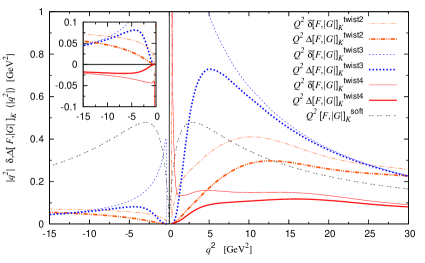
Figure 4: Relative contributions of the soft $\{F,G\}^{\rm soft}_{K}$ (double-dot black lines), twist-2 $\Delta\{F,G\}^{\rm twist2}_{K}$ (thick double-dot dashed orange lines), twist-3 $\Delta\{F,G\}^{\rm twist3}_{K}$ (thick dotted blue lines), and twist-4 $\Delta\{F,G\}^{\rm twist4}_{K}$ (thick solid red lines) terms in Eq. II.2. The same terms without the pre-factor modifications are also displayed.

In the Fig. 4, we plot the individual terms of Eq. II.2, i.e., $\{F,G\}^{\rm soft}_{K}$, $\Delta\{F,G\}^{\rm twist2}_{K}$, $\Delta\{F,G\}^{\rm twist3}_{K}$ and $\Delta\{F,G\}^{\rm twist4}_{K}$, which should give an idea about the relative magnitude of each contribution for intermediate values of $Q^{2}$ up to 30 GeV². For comparison, we also display the results obtained without including the pre-factor modifications, which do not show any appreciable difference for $Q^{2}$ values beyond $\sim 5-10$ GeV². As expected, the standard twist-2 contributions are much smaller compared to the soft QCD and the twist-3 power corrections at moderate-energies. However, the twist-4 contributions are seen to be indeed small (about 1/3 of the magnitude of the twist-2), which are, in fact, negative in the space-like region. In the time-like region, since all the hard contributions are complex, it only makes sense to plot the modulus of the individual twist corrections. It is notable that the general enhancement of all the time-like hard contributions relative to the space-like ones can be attributed to the time-like parton propagators developing poles that are absent in the space-like region. To illustrate this point, it is useful to plot the part of the hard kernel $H_{\pm}(x,y,Q,b_{1},b_{2})$ that is common to all the twist corrections to the hard form factors. Fig. 5 shows the variation of the space- and time-like kernels $H_{\pm}$ (in the impact parameter space) as a function of $Q^{2}$ for some arbitrary fixed values of the parameters $x,y,b_{1}$ and $b_{2}$. It immediately becomes clear that the real-valued space-like kernel $H_{+}$ has a rapidly decaying exponential behavior, whereas the complex-valued time-like kernel $H_{-}$ has rather large amplitude oscillatory real and imaginary components which decay very gradually with increasing $Q^{2}$. In reference to Eqs. 13 and II.1, we note that if $\{x,y\}\ll 1\Rightarrow\{xQ^{2},\,xyQ^{2}\}\sim\{{\mathbf{k}}^{2}_{T},\,{\mathbf{l}}^{2}_{T}\}\ll Q^{2}$, and if $\{x,y\}\sim 1\Rightarrow\{xQ^{2},\,xyQ^{2}\}\sim Q^{2}$, so that the terms in the denominators tend to cancel each other in the time-like but not in the space-like domain. This explains why the amplitude of the time-like oscillations in $H_{-}$ grow larger and larger near the endpoints $x,y\rightarrow 0$.

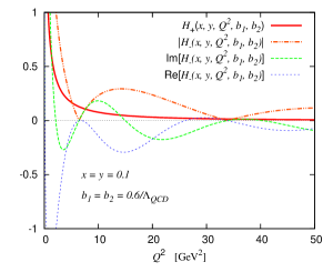
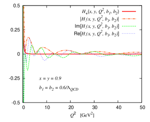
Figure 5: The space- and time-like hard kernels $H_{\pm}(x,y,Q,b_{1},b_{2})$ in the impact space representation for two sets of choices for the collinear momentum fractions with arbitrary fixed $b_{1},b_{2}$: $x=y=0.1$ (left plot) and $x=y=0.9$ (right plot).

The most striking feature of our results in Fig. 4 is the anomalously large twist-3 contribution in the time-like region, similar to what was seen for the pion Raha2 , dominating all the other corrections for the entire range of low- and moderate-energies. This huge asymmetry between the space- and time-like twist-3 contributions comes from the additional parametric enhancement of the twist-3 DAs due to the chiral parameter $\mu_{K}$ which makes them particularly sensitive to the chiral scale. It is the combination of this parametric enhancement along with the occurrence of the time-like poles in the hard kernel that leads to such a characteristic anomalous twist-3 behavior which is completely missing in the twist-2 or even in the twist-4. At this point, one may also worry about possible large contributions from the 3-particle twist-3 sector (related to the 2-particle twist-3 sector through QCD equations of motion) that was not considered in this work. Here, we note that such a possibility can safely be precluded since the 3-particle twist-3 DA receives large parametric suppression from the non-perturbative parameter $f_{3K}\approx 0.0045$ GeV², numerically very much smaller compared to the analogous 2-particle twist-3 parameter $\mu_{K}\approx 1.5$ GeV which greatly enhances the contribution from the 2-particle sector.

Further, it is important to note that (a) the “active” soft gluons that may also arise from the 3-particle twist-3 DA or higher twist DAs likewise, bring about additional power corrections and, therefore, can be safely neglected at large-$Q^{2}$ values, and (b) the “long distance” soft gluons that may be a possible source of the breakdown of TMD factorization, can not probe the small “color-dipole” configurations of the $q\bar{q}$ hadronic bound state at high enough $Q^{2}$ (color-transparency). The remaining collinear gluons are assumed to be effectively tackled within the present TMD factorization scheme, where the inclusion of the 2-particle twist-3 corrections indeed turn out to be the most crucial aspect at the moderate-$Q^{2}$ regime. Note, however, that all such non-perturbative power corrections including the soft contributions rapidly fall-off with increasing $Q^{2}$, and beyond $\sim 50-100$ GeV² the standard twist-2 terms start dominating the asymptotic regime, yielding back numerically the bona fide asymptotic behavior given by the Farrar and Jackson result FJ .

$$\{F,G\}^{\rm asy}_{K}(Q^{2})=\frac{8\pi\alpha_{s}(Q^{2})f^{2}_{K}}{Q^{2}}\,.$$ (38)

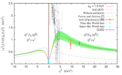
Figure 6: The total scaled kaon form factors, denoted by the thick solid (red) lines; the soft form factors $\{F,G\}^{\rm soft}_{K}$, denoted by the double-dot (black) lines; and the asymptotic QCD result FJ , denoted by the short-dashed (orange) lines. The shaded area is our estimated theoretical error. The experimental data taken from ee-hh ; CLEO and the phenomenological result Seth is shown for comparison.

Our final prediction for the total scaled electromagnetic kaon form factors $\{F,G\}_{K}$ (from Eq. II.2) up to twist-4 accuracy in the range of intermediate energies/momentum transfers is presented in Fig. 6, along with the result for the soft form factors $\{F,G\}^{\rm soft}_{K}$ and the standard asymptotic QCD result of Farrar and Jackson FJ for comparison. To estimate the theoretical error we studied the variation of the wavefunction parameters provided in the Tables 1 and 2. In addition, we varied the chiral parameter $\mu_{K}=m^{2}_{K}/(m_{u}+m_{s})$ which is often taken to be slightly lower $\sim 1.3-1.5$ GeV in the literature Raha1 ; Raha2 ; Keum ; Sanda ; Li ; Lu ; Ball ; B-decay ; CHPT than its naive value about 1.7 GeV expressed in terms of the current quark masses. In this analysis, we take $\mu_{K}=1.5\pm 0.2$ and include its variation in the error estimate. The shaded area, thus obtained, can be regarded as our rough estimate for the theoretical error, where the solid (red) curve corresponds to the central values of the parameters. While our result is relatively insensitive to the choice of the parameters in the space-like region, the time-like result turns out to be very sensitive to the choice of $\mu_{K}$ whose variation alone amounts for more than $90\%$ of the error-bar. The error due to the rest of the model parameters is generously overestimated to include possible uncertainties due to the soft parts which we do not a priori  take into account. Thus, we should stress that our pQCD based error estimate in the low-$Q^{2}$ region (which apparently looks small) must be considered in a very conservative sense and can not be taken seriously below $\sim 5$ GeV². A more rigorous error analysis is impossible at the moment due to poor quality of the experimental data.

Several comments are now in order:

• The width of our error-bar is large enough to completely subsume effects due to further inclusion of higher-twists (e.g., twist-5 and twist-6), sub-leading Fock states and higher helicity components whose contributions should be tiny, not exceeding even 1%.

• Our LO (in $\alpha_{s}$) scattering kernels are apparently gauge dependent arising from the contributions of the single hard gluon propagator. However, in the context of the $\pi\gamma^{*}\rightarrow\gamma$ transition form factor, it can be shown through a systematic order by order calculation using $k_{T}$-factorization that there is indeed a cancellation of the gauge dependences between the quark-level diagrams of the hard kernel and the effective diagrams of the pion wavefunction Nandi , so that the net result turns out to be gauge-invariant to all orders. It is, thus, believed that the same technique can be straightforwardly extended to other hadronic elastic and transition form factors, including the present context of the kaon form factors, at least up to the level of NLO corrections.

• The factorized hard form factors further suffer from renormalization/factorization scale dependent ambiguities that typically emerge from the truncation of the perturbative series and would be absent if we were able to obtain an all-order result in the QCD coupling $\alpha_{s}$. To minimize the scale dependence in our present investigation, we adhere to a fixed prescription with the scales set to the momentum transfer $Q$ Coriano ; Nandi , as mentioned previously in the context of the Sudakov factor. In this way, we hope to improve the reliability and self-consistency of the perturbative prediction and reduce the influence from higher-order corrections.

• Nevertheless, a naive estimation of the NLO twist-2 contributions to the kaon form factors, using available NLO calculations for the pion form factor in asymptotic QCD, can be roughly expressed as NLO

  $$Q^{2}\{F,G\}^{\rm NLO}_{K}\approx(0.903\,{\rm GeV}^{2})\,\alpha^{2}_{s}(Q^{2})\,\frac{f^{2}_{K}}{f^{2}_{\pi}}\,,$$ (39)

  which yields a rather nominal contribution $\sim 20-30\%$ that is roughly of the same order of magnitude as the twist-4 contributions obtained in our analysis. It is to be noted that the above estimation is based on the usual collinear factorization approach NLO which did not take TMD into account. Including the $k_{T}$ dependence of the kernel might further reduce the NLO corrections, as was shown in the cases of the pion k_T_pi and the nucleon k_T_N form factors. It goes without saying that a full systematic NLO calculation (including twists-3) within the TMD factorization scheme, which is missing until now, would be indispensable in resolving this issue about the definitive magnitude of the sub-leading corrections.

On the experimental side, as seen in Fig. 6, currently the space-like region is completely devoid of data points at $Q^{2}$ values higher than $\sim 0.2$ GeV². This makes it difficult, if not impossible, to compare such low-energy data with our predictions based on a pQCD approach which becomes unreliable and diverges rapidly in the vicinity of the Landau pole $\Lambda_{\rm QCD}\approx 0.2$ GeV. For the time-like region, there existed some older kaon data at relatively higher energies but with very poor statistics ee-hh . For such measurements the data above $Q^{2}>4.7$ GeV² had either upper limits or errors $\geq 50\%$. However, the recent CLEO measurements CLEO at $Q^{2}=13.48$ GeV², apparently with a very small error-bar of $\pm 15\%$, can provide first possible opportunity to critically test theoretical predictions, although they do not shed light on the variation with $Q^{2}$, which is a distinguishing feature of our result. Clearly, not only the moderate-energy time-like data seems reasonably reconciled, at higher energies both the CLEO result and the recent phenomenological prediction from $J/\psi$ decays: $M_{J/\psi}^{2}\left|G_{K}(M_{J/\psi}^{2}\!=\!9.59\,\mathrm{GeV}^{2})\right|=0.81\pm 0.18$ GeV² Seth , lie within reasonable range of our prediction for the total time-like form factor. This is surprisingly consistent with the pion form factor results presented in Raha2 , also obtained within the light-cone $k_{T}$-factorization approach, that agreed well with most of the available moderate-energy data (with statistics far better than the kaon data), including the CLEO data and a similar phenomenological prediction Milana based on $J/\psi$ decay analysis. Note that in the analysis Raha2 , the central value of the twist-3 chiral parameter $\mu_{\pi}$ was also taken to be 1.5 GeV.

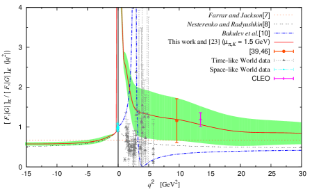
Figure 7: Variation of the ratio of the pion and kaon time-like form factors with $Q^{2}$ in different approaches. The pion and kaon experimental data are taken from pion_exp ; ee-hh ; CLEO ; kaon_exp_space .

To this end, we consider the pion to kaon form factor ratios. In Fig. 7, using the central result for the pion form factors from Raha2 (with $\mu_{\pi}=1.5$ GeV) we plot its variation with $Q^{2}$. The theoretical errors of the present work and Raha2 are added in quadrature to obtain the error band as shown in the figure. The large error should not come as a surprise as the errors of both the pion and kaon factors are large. We now compare this result with other theoretical predictions and available experimental data. Note that the standard asymptotic pQCD result of Farrar and Jackson FJ yields a $Q^{2}$ independent ratio,

$$\left|\frac{\{F,G\}^{\rm asy}_{\pi}(Q^{2})}{\{F,G\}^{\rm asy}_{K}(Q^{2})}\right|=\frac{f^{2}_{\pi}}{f^{2}_{K}}=0.67\,.$$ (40)

Clearly, the central value of our time-like ratio deviates appreciably from the asymptotic value at low- and moderate-$Q^{2}$, but however, it gradually approaches the asymptotic value at large $Q^{2}$, and so does the space-like ratio. While our prediction fails to agree with the very low-energy time-like data points ee-hh , showing the limitations of pQCD at such low-$Q^{2}$ values, the higher $Q^{2}\sim 4$ GeV² data points can somewhat be accommodated within our error-bars. At the same time, our time-like ratio at $Q^{2}=13.48$ GeV², i.e.,

$$\left|\frac{G_{\pi}(13.48\,{\rm GeV}^{2})}{G_{K}(13.48\,{\rm GeV}^{2})}\right|=1.06\pm 0.46\,,$$ (41)

is surprisingly close to the CLEO value: $1.19\pm 0.17$ at $Q^{2}=13.48$ GeV² CLEO , and the result obtained by taking the ratio of the phenomenologically estimated time-like pion form factor Milana and the time-like kaon form factor Seth , with the respective errors again added in quadrature:

$$\left|\frac{G_{\pi}(M^{2}_{J/\psi}=9.48\,{\rm GeV}^{2})}{G_{K}(M^{2}_{J/\psi}=9.48\,{\rm GeV}^{2})}\right|=1.16\pm 0.55$$ (42)

It is also noteworthy mentioning that the recent analysis DFM based on a Light-Front Covariant Model (LFCM) up to $-q^{2}=10$ GeV², yielded the ratio of the form factors quite similar to what we obtain in the space-like region. Finally, in Fig. 7, we compare our result, evidently working better towards large-$Q^{2}$ values, with the soft QCD results obtained from QCDSR which are instead known to yield reliable predictions at low- and moderate-$Q^{2}$ values. For example, the plot corresponding to the LD result Nest not only agrees well with the very low-$Q^{2}$ space-like data (not resolved in the figure), but also with the low-energy time-like data when naively used in the time-like region. While, the analytically continued time-like LD result (see, Eq. 28) Stefanis1 at low-energies yields a plot very different from that of Nest , but toward larger-$Q^{2}$ values both yield very similar predictions. Nevertheless, the QCDSR results significantly differ from the CLEO result and the one obtained from the phenomenological $J/\psi$ decay analysis. It is to be noted that in spite of the additional inclusion of the hard contributions, our space-like ratio of the total form factors does not differ significantly from that of Nest , except at the very low-$Q^{2}\sim 0.2$ GeV² below which our result rapidly blows up.

To sum up, in this paper we tried to systematically study the higher twist effects, namely, the twist-3 and twist-4 corrections to the standard twist-2 pQCD charged kaon form factors by adopting minimal model dependence arising from the inclusion of (a) the transverse degrees of freedom in the kaon wavefunctions/DAs, and (b) the non-factorizable soft QCD corrections via local duality. The work presented here extends and completes the analyses of the previous work Raha1 ; Raha2 . Assuming the validity of the $k_{T}$-factorization ansatz through the explicit TMD of the scattering kernel, we showed a non-trivial twist-3 contribution in the 2-particle sector which along with the large soft QCD corrections turn out to be the real hallmark of the “modified pQCD + soft QCD” approach to determine the space- and time-like kaon form factors. Other correction such as the 2-particle twist-4 were explicitly shows to have minor contributions only. To this end, the available moderate-energy experimental kaon data seems to be reasonably reconciled with the range of our predictions. It is also reassuring that the same approach works equally well independently for the electromagnetic pion form factors, which adds confidence to the arguments used in obtaining our results. It may, therefore, be speculated why the factorized result works so well for both the pion and kaon form factors in obtaining estimates, at least in the correct “ball-park”, in spite of factors like the resonances, hadronization and other final state interaction, naively neglected in this approach, that may render the factorized pQCD result questionable at the presently probed phenomenological region. However, to draw definite conclusion it is invaluable to have more high precision intermediate energy data, rather than to base our conclusions on such poor quality data.

Acknowledgments: The authors would like to thank J.-W Chen and H.-N. Li and N.G. Stefanis for various discussions.

IV Appendix

2-particle Collinear Distribution Amplitudes (DAs)

The 2-particle twist-3 collinear DAs for the charged kaon (say, $K^{-}$) are defined at the scale of $\mu_{0}\approx 1$ GeV, in terms of the following non-local matrix elements Filyanov ; Ball ; Lenz :

$$\langle 0|\bar{u}(z)\,i\gamma_{5}\,s(-z)|K^{-}(P)\rangle\!\! = \!\!\mu_{K}\int^{1}_{0}dx\,e^{i\xi(Pz)}\phi^{\,p}_{3;K}(x,\mu_{0}^{2})\,,$$ (1)

$$\langle 0|\bar{u}(z)\,\sigma_{\alpha\beta}\gamma_{5}\,s(-z)|K^{-}(P)\rangle\!\! = \!\!-\frac{i}{3}\,\mu_{K}\left\{1-\left(\frac{m_{u}+m_{s}}{m_{K}}\right)^{2}\right\}$$

$$\times\,(P_{\alpha}z_{\beta}-P_{\beta}z_{\alpha})\,\int^{1}_{0}dx\,e^{i\xi(Pz)}\phi^{\sigma}_{3;K}(x,\mu_{0}^{2})$$

with $\mu_{K}=m^{2}_{K}/(m_{u}+m_{s})$ and $\xi=2x-1$. Note that the gauge-link factors (Wilson-line) in the matrix elements are to be implicitly understood. The normalization conditions for the above twist-3 DAs are given by

$$N^{\,p,\sigma}_{3;K}=\int^{1}_{0}\,dx\,\phi^{\,p,\sigma}_{3;K}(x,\mu^{2})=\frac{f_{K}}{2\sqrt{2N_{c}}}\,,$$ (2)

which have the following asymptotic forms:

$$\phi^{{p}\,({\rm as})}_{3;K}(x)\!\! = \!\!\frac{f_{K}}{2\sqrt{2N_{c}}}\,,$$

$$\phi^{{\sigma}\,({\rm as})}_{3;K}(x)\!\! = \!\!\frac{3f_{K}}{\sqrt{2N_{c}}}\,x(1-x)\,.$$ (3)

The explicit formulas for the non-asymptotic 2-particle twist-3 collinear DAs, expressed as a series expansion over conformal spins at next-to-leading order, are given by Ball

$$\phi^{p}_{3;K}(x,\mu^{2})\!\! = \!\!\phi^{{p}\,({\rm as})}_{3;K}(x)\left\{1+\left(30\eta_{3K}(\mu^{2})-\frac{5}{2}\,\rho^{2}_{K}(\mu^{2})\right)C^{1/2}_{2}(\xi)\right.$$

$$+\left.\left(-3\eta_{3K}(\mu^{2})\,\omega_{3K}(\mu^{2})-\frac{27}{20}\,\rho^{2}_{K}(\mu^{2})-\frac{81}{10}\,\rho^{2}_{K}(\mu^{2})\,a^{K}_{2}(\mu^{2})\right)C^{1/2}_{4}(\xi)\right\}\,,$$

$$\phi^{\sigma}_{3;K}(x,\mu^{2})\! = \!\phi^{{\sigma}\,({\rm as})}_{3;K}(x)\left\{1+\left(5\eta_{3K}(\mu^{2})-\frac{1}{2}\eta_{3K}(\mu^{2})\,\omega_{3K}(\mu^{2})\right.\right.$$ (4)

$$-\left.\left.\frac{7}{20}\,\rho^{2}_{K}(\mu^{2})-\frac{3}{5}\,\rho^{2}_{K}(\mu^{2})\,a^{K}_{2}(\mu^{2})\right)C^{3/2}_{2}(\xi)\right\}$$

with

$$\eta_{3K}=\frac{f_{3K}}{f_{K}}\frac{1}{\mu_{K}}\quad;\quad\rho_{K}=\frac{m_{K}}{\mu_{K}}\,,$$

the non-perturbative parameters $f_{3K}$ and $\omega_{3K}$ being defined through the following matrix elements of local twist-3 operators:

$$\langle 0|{\bar{u}}(0)\,\sigma_{\mu\nu}\gamma_{5}\,g_{s}G_{\alpha\beta}\,s(0)|K^{-}(P)\rangle=if_{3K}\left(P_{\alpha}P_{\mu}g_{\nu\beta}-P_{\alpha}P_{\nu}g_{\mu\beta}-P_{\beta}P_{\mu}g_{\nu\alpha}+P_{\beta}P_{\nu}g_{\alpha\mu}\right)\,,$$

$$\langle 0|{\bar{u}}(0)\,\sigma_{\mu\lambda}\gamma_{5}[iD_{\beta},g_{s}G_{\alpha\lambda}]\,s(0)\!\! - \!\!\frac{3}{7}\,i\partial_{\beta}\,{\bar{u}}(0)\,\sigma_{\mu\lambda}\gamma_{5}\,g_{s}G_{\alpha\lambda}\,s(0)|K^{-}(P)\rangle$$ (5)

$$=\frac{3}{14}\,if_{3K}P_{\alpha}P_{\beta}P_{\mu}\,\omega_{3K}+{\mathcal{O}}(\rm higher\,\,twist)\,,$$

where $g_{s}$ is the strong coupling and $G_{\alpha\beta}$ is the gluon field tensor. The LO scale dependence of various twist-3 parameters are given by

$$\rho_{K}(\mu^{2})\! = \!L^{\gamma^{(0)}_{3;s{\bar{u}}}/\beta_{0}}\,\rho_{K}(\mu^{2}_{0})\,;\quad\gamma^{(0)}_{3;s{\bar{u}}}=1\,,$$

$$\eta_{3K}(\mu^{2})\! = \!L^{\gamma^{(0)}_{3;\eta}/\beta_{0}}\,\eta_{3K}(\mu^{2}_{0})\,;\quad\gamma^{(0)}_{3;\eta}=\frac{4}{3}\,{\mathcal{C}}_{F}+\frac{1}{4}\,{\mathcal{C}}_{A}\,,$$

$$\omega_{3K}(\mu^{2})\! = \!L^{\gamma^{(0)}_{3;\omega}/\beta_{0}}\,\omega_{3K}(\mu^{2}_{0})\,;\quad\gamma^{(0)}_{3;\omega}=-\frac{7}{24}\,{\mathcal{C}}_{F}+\frac{7}{12}\,{\mathcal{C}}_{A}\,,$$

$$a^{K}_{1}(\mu^{2})\! = \!L^{\gamma^{(0)}_{1}/\beta_{0}}\,a^{K}_{1}(\mu^{2}_{0})\,;\quad\gamma^{(0)}_{1}=\frac{2}{3}\,{\mathcal{C}}_{F}\,,$$

$$a^{K}_{2}(\mu^{2})\! = \!L^{\gamma^{(0)}_{2}/\beta_{0}}\,a^{K}_{2}(\mu^{2}_{0})\,;\quad\gamma^{(0)}_{2}=\frac{25}{24}\,{\mathcal{C}}_{F}\,,$$ (6)

where $L=\alpha_{s}(\mu^{2})/\alpha_{s}(\mu^{2}_{0})$,  ${\mathcal{C}}_{F}=(N^{2}_{c}-1)/2N_{c}$ and ${\mathcal{C}}_{A}=N_{c}$. However, the strange quark being massive, there is operator mixing of the ones in Eq. (IV) with those of twist-2 operators, so that the resulting LO RG equations give the following scale dependences:

$$f_{3K}(\mu^{2})\! = \!L^{55/36\beta_{0}}f_{3K}(\mu^{2}_{0})+\frac{2}{19}\left(L^{1/\beta_{0}}-L^{55/36\beta_{0}}\right)[f_{K}\,m_{s}](\mu^{2}_{0})$$

$$+\,\frac{6}{65}\left(L^{55/36\beta_{0}}-L^{17/9\beta_{0}}\right)[f_{K}\,m_{s}\,a^{K}_{1}](\mu^{2}_{0})\,,$$

$$\left[f_{3K}\,\omega_{3K}\right](\mu^{2})\! = \!L^{26/9\beta_{0}}[f_{3K}\,\omega_{3K}](\mu^{2}_{0})+\frac{1}{170}\left(L^{1/\beta_{0}}-L^{26/9\beta_{0}}\right)[f_{K}\,m_{s}](\mu^{2}_{0})$$ (7)

$$+\,\frac{1}{10}\left(L^{17/9\beta_{0}}-L^{26/9\beta_{0}}\right)[f_{K}\,m_{s}\,a^{K}_{1}](\mu^{2}_{0})$$

$$+\,\frac{2}{15}\left(L^{43/(18\beta_{0})}-L^{26/9\beta_{0}}\right)[f_{K}\,m_{s}\,a^{K}_{2}](\mu^{2}_{0})\,.$$

The 2-particle twist-4 collinear DAs modify the twist-2 axial matrix element and are given by

$$\langle 0|\bar{u}(z)\,\gamma_{\mu}\gamma_{5}\,s(-z)|K^{-}(P)\rangle\! = \!iP_{\mu}\,\int^{1}_{0}dx\,e^{i\xi(Pz)}\,\left[\phi_{2;K}(x,\mu_{0}^{2})+\frac{1}{4}m^{2}_{K}z^{2}{\mathbb{A}}_{4;K}(x,\mu^{2}_{0})\right]$$ (8)

$$+\frac{i}{2}f_{K}m^{2}_{K}\frac{1}{Pz}z_{\mu}\,\int^{1}_{0}dx\,e^{i\xi(Pz)}\,{\mathbb{B}}_{4;K}(x,\mu_{0}^{2})\,,$$

where ${\mathbb{B}}_{4;K}=g_{4;K}-\phi_{2;K}$, with the normalization conditions expressed as

$$N^{\,{\mathbb{A}},g}_{4;K}=\int^{1}_{0}\,dx\,\{{\mathbb{A}},g\}_{4;K}(x,\mu^{2})=\frac{f_{K}}{2\sqrt{2N_{c}}}\,,$$ (9)

and the asymptotic forms namely,

$${\mathbb{A}}^{({\rm as})}_{4;K}(x)\! = \!\frac{15f_{K}}{\sqrt{2N_{c}}}\,x^{2}(1-x)^{2}\,,$$

$$g^{({\rm as})}_{4;K}(x)\! = \!\frac{f_{K}}{2\sqrt{2N_{c}}}\,.$$ (10)

Next we display the explicit forms of the non-asymptotic twist-4 collinear DAs at NLO in conformal spin Ball :

$${\mathbb{A}}_{4;K}(x,\mu^{2})\! = \!\frac{3f_{K}}{{\mathcal{N}}_{\mathbb{A}}\sqrt{2N_{c}}}\,x(1-x)\left\{\frac{16}{15}+\frac{24}{35}\,a^{K}_{2}(\mu^{2})+20\,\eta_{3K}(\mu^{2})+\frac{20}{9}\,\eta_{4K}(\mu^{2})\right.$$

$$\left.+\left(-\frac{1}{15}+\frac{1}{16}-\frac{7}{27}\,\eta_{3K}(\mu^{2})\,\omega_{3K}(\mu^{2})-\frac{10}{27}\,\eta_{4K}(\mu^{2})\right)\,C^{3/2}_{2}(\xi)+\left(-\frac{11}{210}\,a^{K}_{2}(\mu^{2})\right.\right.$$

$$\left.\left.-\frac{4}{135}\,\eta_{3K}(\mu^{2})\,\omega_{3K}(\mu^{2})\right)\,C^{3/2}_{4}(\xi)\right\}+\frac{f_{K}}{2{\mathcal{N}}_{\mathbb{A}}\sqrt{2N_{c}}}\,\left(-\frac{18}{5}\,a^{K}_{2}(\mu^{2})+21\eta_{4K}(\mu^{2})\,\omega_{4K}(\mu^{2})\right)$$

$$\times\left\{2x^{3}(10-15x+6x^{2})\ln{x}+2\bar{x}^{3}(10-15\bar{x}+6\bar{x}^{2})\ln\bar{x}+x\bar{x}(2+13x\bar{x})\right\}\,,$$

$$g_{4;K}(x,\mu^{2})\! = \!\frac{f_{K}}{2\sqrt{2N_{c}}}\left\{1+\left(1+\frac{18}{7}\,a^{K}_{2}(\mu^{2})+60\,\eta_{3K}(\mu^{2})+\frac{20}{3}\,\eta_{4K}(\mu^{2})\right)\,C^{1/2}_{2}(\xi)\right.$$ (11)

$$\left.+\left(-\frac{9}{28}\,a^{K}_{2}(\mu^{2})-6\,\eta_{3K}(\mu^{2})\,\omega_{3K}(\mu^{2})\right)\,C^{1/2}_{4}(\xi)\right\}\,,$$

where $\bar{x}=1-x$, and in the notation of Filyanov , $\delta^{2}\equiv m^{2}_{K}\eta_{4K}$ and $\epsilon\equiv 21/8\,\omega_{4K}$. Note that the additional factor ${\mathcal{N}}_{\mathbb{A}}\approx 3.5$ in the denominator of ${\mathbb{A}}_{4;K}$ is a contrast to the expression given in Ball , which is introduced to normalize the DA. The non-perturbative parameters $\eta_{4K}$ and $\omega_{4K}$ are defined through the following matrix elements of local twist-4 operators:

$$\langle 0|{\bar{u}}(0)\,\gamma_{\alpha}\,ig_{s}\widetilde{G}_{\mu\nu}\,s(0)|K^{-}(P)\rangle=-\frac{1}{3}f_{K}m^{2}_{K}\eta_{4K}\left(P_{\mu}g_{\nu\alpha}-P_{\nu}g_{\mu\alpha}\right)\,,$$

$$\langle 0|{\bar{u}}(0)\,[iD_{\mu},ig_{s}\widetilde{G}_{\nu\lambda}]\gamma_{\lambda}\,s(0)\!\! - \!\!\frac{4}{9}\,i\partial_{\mu}\,{\bar{u}}(0)\,ig_{s}\widetilde{G}_{\nu\lambda}\gamma_{\lambda}\,s(0)|K^{-}(P)\rangle$$ (12)

$$=\!f_{K}m^{2}_{K}\eta_{4K}\omega_{4K}\left(P_{\mu}P_{\nu}-\frac{1}{4}m^{2}_{K}\,g_{\mu\nu}\right)+{\mathcal{O}}(\rm{twist\,5})\,,$$

where, $\widetilde{G}_{\mu\nu}=\frac{1}{2}\epsilon_{\mu\nu\rho\sigma}G^{\rho\sigma}$ is the dual gluon field tensor. Taking into account the mixing with the operators of lower twists, the LO RG evolution of the twist-4 parameters are

$$\eta_{4K}(\mu^{2})\! = \!L^{\gamma^{(0)}_{4;\eta}/\beta_{0}}\eta_{4K}(\mu^{2}_{0})+\frac{1}{8}\left(1-L^{\gamma^{(0)}_{4;\eta}/\beta_{0}}\right)\,;\quad\gamma^{(0)}_{4;\eta}=\frac{2}{3}\,{\mathcal{C}}_{F}\,,$$

$$\left[\eta_{4K}\,\omega_{4K}\right](\mu^{2})\! = \!L^{\gamma^{(0)}_{4;\eta\omega}/\beta_{0}}\left[\eta_{4K}\,\omega_{4K}\right](\mu^{2}_{0})\,;\quad\gamma^{(0)}_{4;\eta\omega}=\frac{5}{6}\,{\mathcal{C}}_{A}\,.$$ (13)

Finally, we present the various Gegenbauer polynomials used in the above formulas:

$$C^{1/2}_{0}(\xi)\! = \!1\,,$$

$$C^{1/2}_{1}(\xi)\! = \!\xi\,,$$

$$C^{1/2}_{2}(\xi)\! = \!\frac{1}{2}\,(3\xi^{2}-1)\,,$$

$$C^{1/2}_{3}(\xi)\! = \!\frac{1}{2}\,\xi(5\xi^{2}-3)\,,$$

$$C^{1/2}_{4}(\xi)\! = \!\frac{1}{8}\,(35\xi^{4}-30\xi^{2}+3)\,,$$

$$C^{3/2}_{0}(\xi)\! = \!1\,,$$

$$C^{3/2}_{1}(\xi)\! = \!3\xi\,,$$

$$C^{3/2}_{2}(\xi)\! = \!\frac{3}{2}\,(5\xi^{2}-1)\,,$$

$$C^{3/2}_{3}(\xi)\! = \!\frac{5}{2}\,\xi(7\xi^{2}-3)\,.$$ (14)

References

• (1) C. N. Brown et al., Phys. Rev. D 8 (1973) 92; C. J. Babek et al., Phys. Rev. D 17 (1978) 1693; H. Ackermann et al., Nucl. Phys. B 137 (1978) 294; P. Brauel et al., Z. Phys. C 3 (1979) 101; S. R. Amendolia et al., Phys. Lett. B 178 (1986) 435; Phys. Lett. B 277 (1986) 168; J. Volmer, Ph.D. thesis, Vrije Universiteit, Amsterdam, 2000 (unpublished); Phys. Rev. Lett. 86 (2001) 1713; T. Horn et al., Phys. Rev. Lett. 97 (2006) 192001; V. Tadevosyan et al., Phys. Rev. C 75 (2007) 055205.
• (2) M. R. Whalley, J. Phys. G 29 (2003) A1; D. Bollini et al., Lett. Nuovo Cimento 14 (1975) 418.
• (3) T. K. Pedlar et al., Phys. Rev. Lett. 95 (2005) 261803.
• (4) B. Zeidman et al., CEBAF Experiment E91-016/1996; R. Mohring et al., Phys. Rev. Lett. 81 (1998) 1805.
• (5) G. P. Lepage and S. J. Brodsky, Phys. Lett. B 87 (1979) 359; Phys. Rev. Lett. 43 (1979) 545; Phys. Rev. D 22 (1980) 2157; Perturbative Quantum Chromodynamics, A. H. Mueller ed., p.93, World Scientific, Singapore 1989; S. J. Brodsky, in Proceedings of the Quantum Chromodynamics Workshop, La Jolla, California, 1978.
• (6) A. V. Efremov, and A. V. Radyushkin, Phys. Lett. B 94 (1980) 245; Theor. Math. Phys. 42 (1980) 97; A. V. Radyushkin, [arXiv:hep-ph/0410276].
• (7) F. R. Farrar and D. R. Jackson, Phys. Rev. Lett. 43 (1979) 246.
• (8) V. A. Nesterenko and A. V. Radyushkin, Phys. Lett. B 115 (1982) 410.
• (9) N. Isgur and C. H. Llewellyn Smith, Phys. Rev. Lett. 52 (1984) 1080; Nucl. Phys. B 317 (1989) 526; Phys. Lett. B 217 (1989) 535.
• (10) A. P. Bakulev, A. V. Radyushkin and N. G. Stefanis, Phys. Rev. D 62 (2000) 113001.
• (11) N. G. Stefanis, W. Schroers and H.-Ch. Kim, Eur. Phys. J. C 18 (2000) 137.
• (12) A. P. Bakulev, et al., Phys. Rev. D 70 (2004) 033014 [arXiv:hep-ph/0405062].
• (13) B. V. Geshkenbeim and M. V. Terentyev, Phys. Lett. B 117 (1982) 243; Sov. J. Nucl. Phys. 39 (1984) 554; Sov. J. Nucl. Phys. 39 (1984) 873.
• (14) G. A. Miller and J. Pasupathy, Z. Phys. A 348 (1994) 123.
• (15) Z.-T. Wei and M.-Z. Yang, Phys. Rev. D 67 (2003) 094013.
• (16) T. Huang and X.-G. Wu, Phys. Rev. D 70 (2004) 093013 [arXiv:hep-ph/0408252].
• (17) U. Raha and A. Aste, Phys. Rev. D 79 (2009) 034015 arXiv:0809.1359 [hep-ph].
• (18) T. Huang, X.-G. Wu and X.-H. Wu, JHEP 0804:043, 2008 arXiv:0803.4229 [hep-ph].
• (19) Y. Y. Keum, H.-N. Li and A. I. Sanda, Phys. Lett. B 504 (2001) 6; Y. Y. Keum, H.-N. Li, Phys. Rev. D 63 (2001) 054008.
• (20) T. Kurimoto, H.-N. Li and A. I. Sanda, Phys. Rev. D 65 (2002) 014007.
• (21) H.-N. Li, Phys. Rev. D 66 (2002) 094010.
• (22) C. D. Lu, K. Ukai, and M. Z. Yang, Phys. Rev. D 63 (2001) 074009; C. D. Lu and M. Z. Yang, Eur. Phys. J. C 28 (2003) 515.
• (23) J.-W. Chen et al., arXiv:0908.2973 [hep-ph].
• (24) S. D. Drell and T. M. Yan, Phys. Rev.  Lett. 24 (1970) 181; Phys. Rev.  Lett. 24 (1970) 1206.
• (25) V. M. Braun and I. E. Filyanov, Z. Phys. C 44 (1989) 157.
• (26) P. Ball, JHEP 9901 (1999) 010.
• (27) P. Ball, V. M. Braun and A. Lenz, JHEP 0605 (2006) 004 [arXiv:hep-ph/0603063].
• (28) S. J. Brodsky, G. P. Lepage and T. Huang, Invited Talk at the Banff Summer Institute on Particle and Fields (1981), A. Z. Capri and A. N. Kamal, ed., p.143, Plenum Press, New York 1983.
• (29) J. Botts and G. Sterman, Nucl. Phys. B 325 (1989) 62.
• (30) H.-N. Li and G. Sterman, Nucl. Phys. B 381 (1992) 129.
• (31) S. Catani, M. Ciafaloni and F. Hautmann, Phys. Lett. B 242 (1990) 97; Nucl. Phys. B 366 (1991) 135; J. C.Collins and R. K. Ellis, Nucl. Phys. B 360 (1991) 3; E. M. Levin, et al., Sov. J. Nucl. Phys. 53 (1991) 657; T. Huang and Q. X. Shen, Z. Phys. C 50 (1991) 139; J. C. Collins, Acta. Phys. Polon. B 34 (2003) 3103; H.-N. Li and H. S. Liao, Phys. Rev. D 70 (2004) 074030; J. P. Ma and Q. Wang, JHEP 0601 (2006) 067; Phys. Lett. B 642 (2006) 232.
• (32) F. Feng, J. P. Ma and Q. Wang, Phys. Lett. B 674 (2009) 176.
• (33) M. Nagashima and H.-N. Li, Phys. Rev. D 67 (2003) 034001; Eur. Phys. J. C 40 (2005) 395.
• (34) T. Gousset and B. Pire, Phys. Rev. D 51 (1995) 15.
• (35) L. Magnea and G. Sterman, Phys. Rev. D 42 (1990) 4222.
• (36) C. Coriano, H.-N. Li and C. Savkli, JHEP 9807:008 (1998) 008.
• (37) A. P. Bakulev and A. V. Radyushkin, Phys. Lett. B 271 (1991) 223.
• (38) V. L. Chernyak and A. R. Zhitnitsky, Nucl. Phys. B 201 (1982) 492; Nucl. Phys. B 246 (1984) 52; Phys. Rep. 112 (1984) 173.
• (39) K. Seth, Phys. Rev. D 75 (2007) 017301.
• (40) H.-N. Li and H. L. Yu, Phys. Rev. Lett. 74 (1995) 4388; T. W. Yeh and H.-N. Li, Phys. Rev. D 56 (1997) 1615; C. D. Lu and M. Z. Yang, Eur. Phys. J. C 28 (2003) 515.
• (41) A. Pich, arXiv[hep-ph/9806303].
• (42) S. Nandi and H.-N. Li, Phys. Rev. D 76 (2007) 034008.
• (43) B. Melic, B. Nizic and K. Passek, Phys. Rev. D 60 (1999) 074004; in Conference on Nuclear and Particle Physics with CEBAF at Jefferson Laboratory, Dubrovnik, Croatia, 3-10 November 1998, published in Fizika B 8 (1999) 327 [arXiv:hep-ph/9903426].
• (44) R. Jakob and P. Kroll, Phys. Lett. B 315 (1993) 463; ibid. B 319 (1993) 545(E).
• (45) J. Bolz, et al., Z. Phys. C 66 (1995) 267.
• (46) J. Milana, S. Nussinov and M. G. Olsson, Phys. Rev. Lett. 71 (1993) 2533.
• (47) O. A. T. Dias, V. S. Filho and J. P. B. C. de Melo, arXiv:1001.4039v1 [hep-ph].