An attractor for dark matter structures

Abstract

Cosmological simulations of dark matter structures have identified a set of universal profiles, and similar characteristics have been seen in non-cosmological simulations. It has therefore been speculated whether these profiles of collisionless systems relate to accretion and merger history, or if there is an attractor for the dark matter systems. Here we identify such a 1-dimensional attractor in the 3-dimensional space spanned by the 2 radial slopes of the density and velocity dispersion, and the velocity anisotropy. This attractor effectively removes one degree of freedom from the Jeans equation. It also allows us to speculate on a new fluid interpretation for the Jeans equation, with an effective polytropic index for the dark matter particles between $1/2$ and $3/4$. If this attractor solution holds for other collisionless structures, then it may hold the key to break the mass-anisotropy degeneracy, which presently prevents us from measuring the mass profiles in dwarf galaxies uniquely.

1 Introduction

Cosmological dark matter structures which have been formed in an expanding universe appear to have virtually universal profiles. This was first emphasized for the density profile through numerical simulation when Navarro et al. (1996) demonstrated that all structures from galaxies to galaxy clusters are well fitted by the same simple form

$$\rho=\frac{\rho_{0}}{\frac{r}{r_{s}}\left(1+\frac{r}{r_{s}}\right)^{2}}\,,$$ (1)

where $r_{s}$ is the scale radius. Even though various theoretical attempts have been made to explain such density profile (e.g. Henriksen (2007); González-Casado et al. (2007); He & Kang (2010); Hjorth & Williams (2010)) there is still no concensus of the underlying physical reason for this universality.

To ease the task of theoreticians one should look for simple connections in some parameter space. One such connection was suggested by Taylor & Navarro (2001), who presented numerical evidence that the pseudo phase-space density is a power-law in radius

$$\frac{\rho}{\sigma^{3}}\sim r^{-\alpha}\,,$$ (2)

where $\alpha=1.875$ is in agreement with the predictions from the spherical infall model (Bertschinger, 1985). This numerical evidence was soon used in conjunction with the Jeans equation to derive density profiles in general agreement with eq. (1) (Hansen, 2004; Austin et al., 2005; Dehnen & McLaughlin, 2005). One problem does, however, present itself, namely that recent high resolution simulations do not confirm that the pseudo phase-space density is a universal straight line (for recent discussions, see Schmidt et al. (2008); Knollmann et al. (2008); Ludlow et al. (2010)).

In this Letter we study the evolution of pure dark matter structures using numerical simulations. We find that all the various equilibrium dark matter structures, when perturbed in a simple but realistic manner, move towards a particular curve in the 3-dimensional space of the derivatives of density and velocity dispersion, and the velocity anisotropy.

2 Structures in equilibrium

One of the non-trivial aspects of cosmological dark matter structures formed through hierachical mergers in an expanding universe is that they are seldom in perfect equilibrium: the first moment of the collisionless Boltzmann equation, the Jeans equation, is not always exactly obeyed unless all velocity terms are included. When bulk motion can be ignored, this Jeans equation reads (see e.g. Binney (1982))

$$v_{c}^{2}=-\sigma^{2}_{r}\,\left(\gamma+\kappa+2\beta\right)\,,$$ (3)

where we have defined the derivatives of the density and radial velocity dispersion,

$$\gamma\equiv\frac{d{\rm log}\rho}{d{\rm log}r}\,\,\,\,\,{\rm and}\,\,\,\,\,\kappa\equiv\frac{d{\rm log}\sigma_{r}^{2}}{d{\rm log}r}\,,$$ (4)

the velocity dispersion anisotropy is given by

$$\beta\equiv 1-\frac{\sigma_{\rm tan}^{2}}{\sigma^{2}_{\rm rad}}\,,$$ (5)

and the circular velocity is

$$v_{c}^{2}=\frac{GM_{\rm tot}}{r}\,.$$ (6)

Numerical simulations of galaxies or clusters of galaxies often have differences between the left and right hand sides of eq. (3), of the order $20\%$ for large parts of the structures.

This problem can be avoided by manually setting up structures in equilibrium. There are several ways of setting up structures which obey the Jeans equation. The first is the Eddington method, which for a given assumed density profile creates a unique ergodic structure i.e. depending only on the energy of the particles, and hence having $\beta=0$ by definition (Eddington, 1916; Binney, 1982). This method gives the exact distribution function, $f(\mathcal{E})$, and is therefore often stable when evolved by an N-body simulation. When we discuss stable configurations, we intend structures whose profiles, $\rho(r),\sigma_{r}^{2}$ and $\beta(r)$, remain unchanged when evolved for several dynamical times by an N-body code.

The other method is to make an assumption for the radial profiles of the density and velocity anisitropy, and then solve the Jeans equation to get $\sigma_{r}^{2}$ (Hernquist, 1993). In this method the velocity distribution function is assumed to be a Gaussian, and the system will therefore not be exactly stable when evolved by an N-body simulation. However, after having run for a number of dynamical times, such structures settle down in an equilibrium configuration, which often has a fair resemblance to the original density and velocity anisotropy profiles. Below we will use both methods of defining initial conditions.

3 Flow towards an attractor

The Jeans equation in eq. (3) has infinitely many solution: there are 3 unknown functions, $\rho(r),\sigma_{r}^{2}(r)$ and $\beta(r)$, and only one equation. It is therefore no mystery that one can create a wide range of different structures, with different density and velocity profiles, which all obey the Jeans equation. The question we are posing here is, if all these structures, if perturbed in a simple way, will flow to new points in a large volume in solution space, or if there is one or several attractors which the structure will be drawn towards.

As solution space it is natural to consider the 4 dimensional space spanned by $r,\gamma,\kappa$ and $\beta$, see eq. (3). Whereas the Jeans equation allows solutions to fill a large 3-dimensional volume, then if an attractor does exists, we should expect all final structures to land on a low dimensional sheet, potentially a line. In practice we divide each structure into radial bins. For each radial bin we can derive $\gamma,\kappa$ and $\beta$, and this radial bin thus represents a point in 3d space. In this way we also avoid any potential problems concerning scaling different structures in radius.

During the formation of cosmological structures in the real universe, these are continuously being perturbed through the process of mergers. This implies that if an attractor exists in solution space, then we might expect repeated perturbations, such as the ones from ongoing mergers, to support the flow of the structures towards the attractor.

In order to mimic the perturbations of the mergers in a controlled way, we perturb the equilibrated structure in a simple yet fairly realistic manner. The velocity of each particle is multiplied by a random number, in such a way that any given radial bin has exact conservation of kinetic energy and angular momentum. We assure that no particles get a velocity above the escape velocity. Naturally, the potential energy is also conserved during the perturbations. Now, having perturbed each particle in the structure in this controlled manner, we start the N-body code, and let the structure settle into a new equilibrium condition. We let each simulation run for a time corresponding to one dynamical time, $t_{\rm dyn}=1/\sqrt{G\rho}$, at radius 13 times the scale radius.

The simulations were performed with the public version of Gadget-2 (Springel, 2005; Springel et al., 2001) which is a massively parallel N-body code that uses a hierarchical tree algorithm to calculate gravitational forces, and gives individual timesteps to all particles. A spline softening of $0.005r_{s}$ was used. We are being overly conservative in the analysis, and include only regions outside of 5-10 times this softening. We also require that the bins contain at least $5000$ particles.

4 The wide range of initial conditions

In order to allow the systems to start from a large range of initial conditions, we initiate a set of significantly different systems. Using the Eddington method, we have an isotropic system, which has a density profile like a Hernquist profile (Hernquist, 1990), with inner and outer density slopes of $-1$ and $-4$. We construct a cored profile, with central slope of $0$, and outer slope of $-5$. We also use a hoovering profile, $\rho\sim 1/(1+(r/r_{1})^{2}\,(1+r/r_{2})^{3})$, where $r_{1}=0.01$ and $r_{2}=100$ which is characterized by having a large part of the central structure where the slope is $-2$. We also create a set of initial conditions with Osipkov-Merrit anisotropies (Osipkov, 1979; Merritt, 1985) with the property $\beta(r)=1/(1+(r_{a}/r)^{2})$: a Hernquist density profile (slope $-1,-4$) with $r_{a}=1$, and a cored profile (slope $0,-3.5$) with $r_{a}=1.5$. Using the gaussian method, we create 4 structures, with both trivial and highly non-trivial $\beta(r)$ profiles, all with a Hernquist density profile (slope $-1,-4$). All structures presented here contain $10^{6}$ DM particles, and low resolution runs with $10^{5}$ particles establish that this is sufficient for our purpose. All of these initial conditions (after having run for 3 dynamical time at radius 13 times the scale radius) are presented in figure 1. This figure shows that our initial conditions span a large part of the solution space of ($\beta,\gamma+\kappa$). The Jeans equation allows all of this parameter space to be populated, however, there are no initial conditions in the upper right corner, where the inequality $\beta<-\gamma/2$ (An & Evans, 2006) prevents any stable solutions (see also Ciotti & Morganti (2010)).

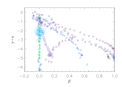
Figure 1: The initial conditions. A 2-dimensional projection in solution space to the Jeans equation. According to the Jeans equation, eq. (3), all points in this space may be populated. No stable solutions exist in the upper right corner. Our various initial conditions of equilibrated structure are created to span a large volume in the 3-dim solution space. All the structures of this figure are in equilibrium, and are stable when evolved in an N-body simulation.

5 The perturbations

All perturbations follow the repeated pattern of kick-flow. First the structure is perturbed (kicked) and then the N-body simulation allows it to settle into (flow towards) a new equlibrium configuration. This kick-flow is repeated numerous times.

We first consider 2 structures, each with initial Hernquist profile and with $\beta=0$. These are created using the Eddington and the Gaussian method respective. We then perturb the energies of each individual particle in the range $[0.75,1.25]$, in such a way that there is energy conservation at each radial bin. The structure is then evolved with Gadget-2 for 1 to 3 dynamical time at 13 times the scale radius. This process is repeated approximately 20 times. The final structures are compared, and we find no significant difference when plotted in the plane ($\beta,\gamma+\kappa$). This shows that there is virtually no dependence in the final result on the method of creating the initial conditions (Eddington vs. Gaussian).

We then take the isotropic Hernquist structure, using the Eddington method, and perturb by changing energies in the much larger range $[0.25,1.75]$. Also this structure ends in the same region in ($\beta,\gamma+\kappa$) after repeated perturbations. This demonstrates that the magnitude of the perturbation is not crucial to the final structure. We also test perturbations where we don’t prevent velocities above the escape velocity: for these structures some particles do leave the structure, and these perturbations are therefore less conservative. Also structures perturbed in this way land on the same curve in solution space. We can therefore perturb all structures by changing energies in the range $[0.25,1.75]$, irrespective of the method of creating the initial conditions.

The result of all these perturbations is presented in figure 2, from which it is clear, that all the structures end up along a 1-dimensional curve in this 2-dim parameter space. It is important to emphasize that we had initial conditions both above and below this attractor solution. When we plot in the 3-dim space spanned by $\gamma,\kappa,\beta$ we still find that the attractor solution spans a non-trivial 1-dim curve.

This curve is clearly S-shaped, but we can approximate it with a piecewise straight line, which for small $\beta$ could be $(\gamma+\kappa)=-8\beta$, and for intermediate $\beta$ it looks like $(\gamma+\kappa)=-0.7-4\beta$. It is interesting to note that the anisotropy-slope connection suggested by Hansen & Moore (2006) looks like $(\gamma)=-0.8-5\beta$ in the region which can be trusted, namely $-2.5<\gamma<-1$ (Hansen & Stadel, 2006; Zait et al., 2008; Navarro et al., 2010), which is in good agreement with our findings. For very high $\beta$ we are in the very outer region of the structures, where full equilibrium can be questioned, since a larger spread in the final points is observed. The included points have been allowed to equlibrate at least 20 dynamical times in total, however, the outermost points have only been allowed 1 dynamical times since the last perturbation. We therefore won’t speculate on the form of the attractor there.

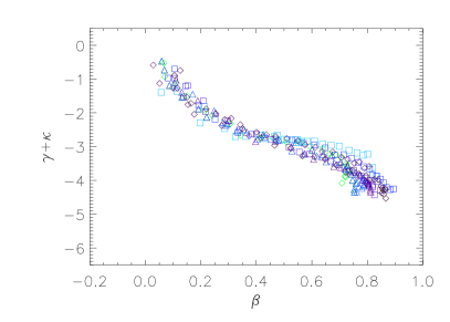
Figure 2: The attractor solution. The same 2-dimensional projection in solution space of the Jeans equation, eq. (3), as presented in Fig. 1. The points represent the final profiles for all the initial conditions, after these have been perturbed and allowed to equilibrate repeatedly. This attractor solution is also a 1-dim curve in the full 3-dim space spanned by $\gamma,\kappa$ and $\beta$.

Whereas the 1-dimensional attractor has a non-trivial S-shape in the space of $\gamma,\kappa$ and $\beta$, then it happens to lie in a simply parametrized sheet, given by one single free parameter, $\delta=0.15$,

$$\beta=\frac{Y}{\left(1+Y^{3}\right)^{\frac{1}{3}}}$$ (7)

where $Y=-\delta\gamma-(1-\delta)\kappa$. This means that when seen in a slightly different projection, the attractor in fig. (2) looks like a very simple curve.

With this attractor we can effectively remove one degree of freedom from the Jeans equation: for a given density profile there is now a unique connection between $\kappa$ and $\beta$, which allows us to calculate both.

6 An effective equation of state

The Jeans equation describing collisionless particles is fundamentally different from the Euler equation for collisional fluids, however, a standard mapping between the two is made by setting $\beta=0$ and interpreting $m\sigma^{2}_{r}/2$ as a temperature (Binney & Tremaine, 1987). The non-trivial part of this interpretations is to assume that $\beta=0$, since numerical simulations for years have demonstrated that $\beta$ is not generally zero (Carlberg et al., 1997; Cole & Lacey, 1996).

We now allow ourselves to use our newly found connection to make a different interpretation of the Jeans equation from a fluid perspective.

Let us first consider the region with small $\beta$, where the attractor solution approximately reads $(\gamma+\kappa)=-8\beta$. When we insert this into the Jeans equation, we get

$$\frac{GM_{\rm tot}}{r}=-\sigma^{2}_{r}\,A\,\left(\gamma+\kappa\right)\,,$$ (8)

where $A=3/4$. If we attempt to describe the dark matter by an effective equation of state (generalizing a polytropic index) we have

$$P=b\,\left(\rho\sigma_{r}^{2}\right)^{K_{0}}\,,$$ (9)

where $b$ is a constant. Thus, if we require that the Jeans equation, eq. (8), should take the form of the equation of hydrostatic equilibrium, $GM/r^{2}=\nabla P/\rho$, then we find the solution $K_{0}=3/4$. We can therefore interpret this by the DM behaving like a fluid with an effective polytropic index of $3/4$.

For intermediate $\beta$ we found approximately the connection $(\gamma+\kappa)=-0.7-4\beta$. This is almost solved in the same way, finding an effective polytropic index of $1/2$, however, the constant term ($B=-0.7$) changes the picture. In order to solve for such an effective polytropic index, we generalize eq. (9) to $P=b\,\rho^{K_{1}}\,\sigma_{r}^{2K_{2}}$, where $b$ is a new constant. We now need to introduce an assumption about the pseudo phase-space density, namely $\rho/\sigma_{r}^{\epsilon}\sim r^{-\alpha}$. Doing this we find the solution, $K_{1}=1/2-B/\alpha$, and $K_{2}=1/2+B\epsilon/2\alpha$.

7 Will any perturbation do?

A ball will always run downhill, if kicked randomly by a group of children playing, however, if they consistently kick the ball uphill, then the ball may appear to defy the attractiveness of gravity. We should expect the same to be possible with the abovefound attractor. In order to quantify this idea we tried to perturb only the radial velocity component. When the radial component is perturbed by a random number (always obeying exact energy conservation in any radial bin) then the radial velocity distribution gets flattend out. When we subsequently let the system evolve by the N-body simulation, the high energy tail of the distribution essentially gets cut off, and thereby the effective radial dispersion gets slightly smaller. When we repeatedly perform such kick-flow, we even manage to get negative values of $\beta$ at intermediate radii. This confirms our expectation that perturbations may be invented, which will defy the attractor. If we instead only perturb the tangential velocities, then the system flows towards the attractor.

We see from this discussion that it is relevant to consider which kind of perturbations should happen during structure formation. During merging there will be violent relaxation. Two salient features of violent relaxation is that it changes the energy of individual particles on a timescale similar to the dynamical time (Lynden-Bell, 1967), which for mergers is of the order $R/v$, where $R$ is the size of the smaller merging object and $v$ is its velocity. We are here interested in the energy exchange with specific particles in the larger structure, which has a different timescale from the equilibration of the smaller structure. The other feature is that violent relaxation acts on all particles irrespective of their orientation. In our example above we have an instantaneous exchange of energies between the particles (reminicent of violent relaxation) and then we let the system flow (which provides the needed phase mixing).

In our particular setup, the kicks do not change any properties of the profiles by themselves, and without the kicks there is no effect of the flow. Thus, when interpreted as violent relaxation (kick) and phase mixing (flow), we see that both are needed to move towards the attractor.

Antonov’s laws of stability state that e.g. an isotropic Hernquist structure will remain isotropic when exposed to minor perturbations. These laws are derived under the assumption that the r.h.s. of the Boltzmann equation is zero. Our perturbations act like an instantaneous non-zero term on the r.h.s. of the Boltzmann equation, and we are therefore not violating Antonov’s laws of stability.

Finally, it is worth emphasizing that we find the attractor in the space of $\gamma,\kappa$ and $\beta$. Very specifically, we do not in this work identify one unique density profile, $\rho(r)$. This may be because we are constraining the perturbations to allow very little freedom in modifying the density profile, or it may be because the universality of the density profile (Navarro et al., 1996; Moore et al., 1998) really finds its origin in accretion history (González-Casado et al., 2007).

8 Breaking the mass velocity anisotropy degeneracy

Let us finally discuss what our newly found attractor may do for the mass-velocity anisotropy degeneracy. When we observe the stellar kinematics in a dwarf galaxy we can observe the stellar density and the stellar dispersion. Then, the jeans equation, eq. (3), tells us that for any assumed velocity anisotropy profile for the stars, $\beta(r)$, we can solve for the total gravitating mass. However, if we had assumed a different $\beta(r)$ then we would have found a different total mass profile (Strigari, 2010).

If we for instance consider a Hernquist density profile with a $\beta$ profile in agreement with numerical simulations and observations (Hansen & Piffaretti, 2007; Host et al., 2009; Wojtak & Lokas, 2010), then the reconstructed mass is overestimated by up to $40\%$, if the analysis is made under the simplifying assumption $\beta=0$. Also the derived inner density slope (from the total mass) is systematically found to be more shallow than the true slope is, by up to $10\%$. This means that if the true density slope is $-1$, then we will measure around $-0.95$, if we assumed $\beta=0$ in the analysis.

This may no longer have to be the case. If our attractor solutions also applies to stellar systems in a dwarf galaxy, or to the dynamics of the galaxies in a galaxy cluster, then we have a unique connection between the 3 quantities, $\gamma,\kappa$ and $\beta$. Therefore, if we have measured (accurately) the stellar density and dispersion profiles, then we do in principle know exactly what $\beta(r)$ looks like, and we can then deduce the unique total mass profile.

9 Conclusions

We have identified an attractor solution for dark matter structures. This implies that any dark matter structure which is repeatedly perturbed (e.g. through violent relaxtion during merging) and then allowed to relax (phase mix), will flow towards this 1-dimensional curve in the 3-dimensional space spanned by the 2 radial derivatives of the density and velocity dispersion, and the velocity anisotropy.

This finding provides strong support for the idea that the universalities found in cosmological dark matter structures are a property of gravity, and not simply a result of similar accretion and merger histories of different structures.

This attractor solution effectively removes one degree of freedom from the Jeans equation, giving hope that we will eventually be able to solve the Jeans equations analytically, and thereby truely understand the origin of the universal profiles.

Acknowledgements
It is a pleasure to thank Jens Hjorth for discussions. The simulations were performed on the facilities provided by the Danish Center for Scientific Computing. The Dark Cosmology Centre is funded by the Danish National Research Foundation.

References

- An & Evans (2006) An, J. H., & Evans, N. W. 2006, ApJ, 642, 752
- Austin et al. (2005) Austin, C. G., Williams, L. L. R., Barnes, E. I., Babul, A., & Dalcanton, J. J. 2006, ApJ, 634, 756
- Bertschinger (1985) Bertschinger, E. 1985, ApJS, 58, 39
- Binney (1982) Binney, J. 1982, ARA&A, 20, 399
- Binney (1982) Binney, J. 1982, MNRAS, 200, 951
- Binney & Tremaine (1987) Binney, J., & Tremaine, S. 1987, Princeton, NJ, Princeton University Press, 1987, 747 p.
- Carlberg et al. (1997) Carlberg, R. G., et al. 1997, ApJ, 485, L13
- Ciotti & Morganti (2010) Ciotti, L., & Morganti, L. 2010, MNRAS, 401, 1091
- Cole & Lacey (1996) Cole, S., & Lacey, C. 1996, MNRAS, 281, 716
- Dehnen & McLaughlin (2005) Dehnen, W., & McLaughlin, D. 2005, MNRAS, 363, 1057
- Eddington (1916) Eddington, A. S. 1916, MNRAS, 76, 572
- González-Casado et al. (2007) González-Casado, G.s, Salvador-Solé, E., Manrique, A., & Hansen, S. H. 2007, arXiv:astro-ph/0702368
- Hansen (2004) Hansen S. H. 2004 MNRAS, 352, L41
- Hansen & Moore (2006) Hansen S. H., & Moore B 2006, New Astron., 11, 333
- Hansen & Stadel (2006) Hansen, S. H., & Stadel, J. 2006, Journal of Cosmology and Astro-Particle Physics, 5, 14
- Hansen & Piffaretti (2007) Hansen, S. H., & Piffaretti, R. 2007, A&A, 476, L37
- He & Kang (2010) He, Ping & Kang, Dong-Biao 2010, submitted
- Henriksen (2007) Henriksen, R. N. 2007, arXiv:0709.0434
- Hernquist (1990) Hernquist, L. 1990, ApJ, 356, 359
- Hernquist (1993) Hernquist, L. 1993, ApJS, 86, 389
- Hjorth & Williams (2010) Hjorth, J, & L. Williams, 2010, submitted
- Host et al. (2009) Host, O., Hansen, S. H., Piffaretti, R., Morandi, A., Ettori, S., Kay, S. T., & Valdarnini, R. 2009, ApJ, 690, 358
- Knollmann et al. (2008) Knollmann, S. R., Knebe, A. & Hoffman, Y. 2008, arXiv:0809.1439
- Ludlow et al. (2010) Ludlow, A. D., Navarro, J. F., Springel, V., Vogelsberger, M., Wang, J., White, S. D. M., Jenkins, A., & Frenk, C. S. 2010, arXiv:1001.2310
- Lynden-Bell (1967) Lynden-Bell, D. 1967, MNRAS, 136, 101
- Merritt (1985) Merritt, D. 1985, AJ, 90, 1027
- Moore et al. (1998) Moore, B., Governato, F., Quinn, T., Stadel, J. & Lake G. 1998, ApJ, 499, 5
- Navarro et al. (1996) Navarro, J. F., Frenk, C. S., & White, S. D. M. 1996, ApJ, 462, 563
- Navarro et al. (2010) Navarro, J. F., et al. 2010, MNRAS, 402, 21
- Osipkov (1979) Osipkov, L. P. 1979, Soviet Astronomy Letters, 5, 42
- Schmidt et al. (2008) Schmidt, K. B., Hansen, S. H., & Macciò, A. V. 2008, ApJ, 689, L33
- Springel et al. (2001) Springel, V., Yoshida, N., & White, S. D. M. 2001, New Astronomy, 6, 79
- Springel (2005) Springel, V. 2005, MNRAS, 364, 1105
- Strigari (2010) Strigari, L. E. 2010, Advances in Astronomy, 2010,
- Taylor & Navarro (2001) Taylor, J. E., & Navarro, J. F. 2001, ApJ, 563, 483
- Wojtak & Lokas (2010) Wojtak, R., & Lokas, E. L. 2010, arXiv:1004.3771
- Zait et al. (2008) Zait, A., Hoffman, Y., & Shlosman, I. 2008, arXiv:0711.3791