Magnetohydrodynamic Turbulent Cascade of Coronal Loop Magnetic Fields

Abstract

The Parker model for coronal heating is investigated through a high resolution simulation. An inertial range is resolved where fluctuating magnetic energy $E_{{}_{M}}(k_{\perp})\propto k_{\perp}^{-2.7}$ exceeds kinetic energy $E_{{}_{K}}(k_{\perp})\propto k_{\perp}^{-0.6}$. Increments scale as $\delta b_{{}_{\!\ell}}\simeq\ell^{-0.85}$ and $\delta u_{{}_{\!\ell}}\simeq\ell^{+0.2}$ with velocity increasing at small scales, indicating that magnetic reconnection plays a prime role in this turbulent system. We show that spectral energy transport is akin to standard magnetohydrodynamic (MHD) turbulence even for a system of reconnecting current sheets sustained by the boundary. In this new MHD turbulent cascade, kinetic energy flows are negligible while cross-field flows are enhanced, and through a series of “reflections” between the two fields, cascade more than half of the total spectral energy flow.

The heating of solar and stellar atmospheres is an outstanding astrophysical problem Reale (2010). The solar corona has temperatures ($\gtrsim 10^{6}\,K$) up to three orders of magnitude higher than the underlying photospheric and chromospheric layers, sustained by an energy flux of about $10^{7}\,erg\,cm^{-2}\,s^{-1}$ Withbroe and Noyes (1977).

Most of the coronal x-ray and extreme ultraviolet (EUV) radiation is emitted in loops, bright structures threaded by a strong axial magnetic field connecting photospheric regions of opposite polarity. In the scenario proposed by Parker Parker (1972), magnetic field lines are braided by convective photospheric motions that shuffle their footpoints, leading to the “spontaneous” development of small-scale current sheets where the plasma is heated.

It has long been proposed Einaudi et al. (1996) that this scenario can be regarded as a magnetohydrodynamic (MHD) turbulence problem as photospheric motions stir the magnetic field lines’ footpoints, and these motions are transmitted inside by the field-line tension stirring in this way (anisotropically) the whole plasma akin to a body force. Simulations have indeed revealed that the system exhibits many properties of an authentic MHD turbulent system, including the formation of field-aligned current sheets, power-law spectra for the energies, and power-law distributions for energy release, peak dissipation and duration of dissipative events Dmitruk and Gómez (1997); *Einaudi:1999p707; *Dmitruk:2003p499; Rappazzo et al. (2007); *Rappazzo:2008p344; *Rappazzo:2010p4099. Furthermore in recent papers Rappazzo et al. (2007); *Rappazzo:2008p344 we have developed a phenomenological scaling model for this turbulent cascade where at the large scales nonlinearity is weak (i.e., depleted similarly to Galtier et al. (2000)) and at the small scales strong Goldreich and Sridhar (1995).

However this new, line-tied, turbulent regime is quite distinct from the classical MHD turbulence system where energies are in approximate equipartition, as here fluctuating magnetic energy dominates over kinetic energy throughout the inertial range.

Certainly, this system can also be seen as a set of reconnecting current sheets sustained by the boundaries, and a large fraction of the kinetic energy might be contributed by the magnetic field through reconnection itself rather than from cascading large-scale kinetic energy.

It is therefore crucial to understand if turbulence is an appropriate framework to model this problem, namely, can a set of reconnecting current sheets be described in terms of turbulence? The influence of turbulence on magnetic reconnection is an active research topic (e.g., see Lazarian & Vishniac (1999) for a model), but are energy fluxes in a system where magnetic reconnection plays a prime role similar to those of MHD turbulence? We present here a novel investigation of the energy flows between different scales and fields in Parker’s model in order to determine how different the spectral fluxes are and what properties they share with the standard MHD turbulence case Dar et al. (2001); Alexakis et al. (2005); Aluie and Eyink (2010).

A coronal loop is modeled in Cartesian geometry as a plasma with uniform density $\rho_{0}$ embedded in a strong axial magnetic field $B_{0}$ directed along $z$ (see Rappazzo et al. (2008) for a more detailed description of the model and numerical code). Magnetic field lines are line tied at the top and bottom plates where a large-scale velocity field is imposed. In the perpendicular direction ($x$-$y$) periodic boundary conditions are used. The dynamics are modeled with the (non-dimensional) equations of reduced magnetohydrodynamics (RMHD) Kadomtsev and Pogutse (1974); *Strauss:1976p1438:

$${\displaystyle\partial_{t}\mathbf{u}}+\left(\mathbf{u}\cdot\!\mathbf{\nabla_{{}_{\!\!\perp}}}\!\right)\mathbf{u}=-\mathbf{\nabla_{{}_{\!\!\perp}}}\!P+\left(\mathbf{b}\cdot\!\mathbf{\nabla_{{}_{\!\!\perp}}}\!\right)\mathbf{b}+c_{{}_{\!A}}\partial_{z}\mathbf{b}+\frac{1}{R}\mathbf{\nabla_{{}_{\!\!\perp}}}^{\!\!\!2}\mathbf{u},$$

$$\partial_{t}\mathbf{b}+\left(\mathbf{u}\cdot\!\mathbf{\nabla_{{}_{\!\!\perp}}}\!\right)\mathbf{b}=\left(\mathbf{b}\cdot\!\mathbf{\nabla_{{}_{\!\!\perp}}}\!\right)\mathbf{u}+c_{{}_{\!A}}\partial_{z}\mathbf{u}+\frac{1}{R}\mathbf{\nabla_{{}_{\!\!\perp}}}^{\!\!\!2}\mathbf{b},$$ (1)

with $\mathbf{\nabla_{{}_{\!\!\perp}}}\!\!\cdot\mathbf{u}=\mathbf{\nabla_{{}_{\!\!\perp}}}\!\!\cdot\mathbf{b}=0$. Here gradient and Laplacian operators have only orthogonal ($x$-$y$) components as do velocity and magnetic field vectors ($u_{z}$=$b_{z}$=0), while $P$ is the total (plasma plus magnetic) pressure. $c_{{}_{\!A}}$ is the ratio between the Alfvén velocity of the axial field ($B_{0}/\sqrt{4\pi\rho_{0}}$) and the rms of photospheric velocity ($1\,km\,s^{-1}$) and $R$ is the Reynolds number. In the simulation presented here, $c_{{}_{\!A}}=400$, $R=2000$, and the domain spans $0\leq x,y\leq\ell$, $0\leq z\leq L$, with $\ell=1,L=10$ and $1024^{2}\times 512$ grid points. Given the orthogonal Fourier transform $\mathbf{u}(\mathbf{x}_{{}_{\!\perp}},z)=\sum_{\mathbf{k_{{}_{\!\perp}}}}\hat{\mathbf{u}}(\mathbf{k_{{}_{\!\perp}}},z)\,e^{i\mathbf{k_{{}_{\!\perp}}}\!\!\cdot\mathbf{x}_{{}_{\!\perp}}}$ with $\mathbf{k_{{}_{\!\perp}}}=2\pi\,\mathbf{n_{{}_{\!\perp}}}/\ell$ and $\mathbf{n_{{}_{\!\perp}}}\!\in\mathbb{Z}^{2}$, the shell-filtered field $\mathbf{u}_{{}_{K}}$ is defined as Alexakis et al. (2005)

$$\mathbf{u}_{{}_{K}}(\mathbf{x}_{{}_{\!\perp}},z)=\sum_{\mathbf{n}_{{}_{\!\perp}}\in K}\hat{\mathbf{u}}(\mathbf{k_{{}_{\!\perp}}},z)\,e^{i\mathbf{k_{{}_{\!\perp}}}\!\!\cdot\mathbf{x_{{}_{\!\perp}}}},$$ (2)

i.e., it has only components in the “shell” $K$ with wave numbers K-1$<\!|\mathbf{n_{{}_{\!\perp}}}|\!\leq$K. The boundary photospheric velocities at $z\!=\!0,L$ are given random amplitudes for all wave numbers 3$\leq\!n_{{}_{\!\perp}}\!\leq$4 and then normalized so that the rms value is $1/2$ (see Rappazzo et al., 2008). As a result the forcing boundary velocity has only components in shells 3 and 4.

Figure 1: Magnetic ($E_{{}_{M}}$) and kinetic ($E_{{}_{K}}$) energy spectra as a function of the orthogonal wave number $n_{{}_{\!\perp}}$ ($k_{{}_{\!\perp}}=2\pi n_{{}_{\!\perp}}$). Inset: Increments, velocity increasing at high wave numbers.

Since fields filtered in different shells are orthogonal, and indicating the volume integrals with $\langle...\rangle$, the equations for kinetic and magnetic energies $E_{{}_{u}}^{(K)}=\langle\,\mathbf{u}_{{}_{K}}^{2}/2\,\rangle$, $E_{{}_{b}}^{(K)}=\langle\,\mathbf{b}_{{}_{K}}^{2}/2\,\rangle$ in shell $K$ follow from Eqs. (1):

$$\partial_{t}E_{{}_{u}}^{(K)} = \sum_{Q}\left[\mathcal{T}_{{}_{uu}}^{(Q,K)}+\mathcal{T}_{{}_{bu}}^{(Q,K)}\right]+\frac{S^{(K)}}{2}-\frac{\mathcal{D}_{{}_{u}}^{(K)}}{\mathrm{R}}\quad$$ (3)

$$\partial_{t}E_{{}_{b}}^{(K)} = \sum_{Q}\left[\mathcal{T}_{{}_{ub}}^{(Q,K)}+\mathcal{T}_{{}_{bb}}^{(Q,K)}\right]+\frac{S^{(K)}}{2}-\frac{\mathcal{D}_{{}_{b}}^{(K)}}{\mathrm{R}}$$ (4)

These are obtained as for the three-periodic case Alexakis et al. (2005), except for terms $\propto\partial_{z}$ in Eqs. (1) that contribute the integrated Poynting flux $S^{(K)}$ (the work done by photospheric motions on magnetic field lines’ footpoints) entering the system at the boundaries in shell $K$:

$$S^{(K)}=c_{{}_{\!A}}\left(\int_{z=L}\!\mathrm{d}a\ \mathbf{u}_{{}_{K}}\!\cdot\mathbf{b}-\int_{z=0}\!\mathrm{d}a\ \mathbf{u}_{{}_{K}}\!\cdot\mathbf{b}\right).$$ (5)

This does not cancel out along the nonperiodic axial direction $z$. As photospheric velocities have only components in shells 3 and 4 $S^{(K)}$ vanishes outside these two shells (the injection scale). In similar fashion the dissipative terms $\mathcal{D}_{{}_{u}}^{(K)}=\langle\left|\mathbf{\nabla}\mathbf{u}_{{}_{K}}\right|^{2}\rangle$, $\mathcal{D}_{{}_{b}}^{(K)}=\langle\left|\mathbf{\nabla}\mathbf{b}_{{}_{K}}\right|^{2}\rangle$ contribute only at dissipative scales with large $K$.

Between the injection and dissipative scales only the following terms contribute:

$$\mathcal{T}_{{}_{uu}}^{(Q,K)}=-\langle\,\mathbf{u}_{{}_{K}}\!\cdot\left(\mathbf{u}\cdot\mathbf{\nabla}\right)\mathbf{u}_{{}_{Q}}\,\rangle$$ (6)

$$\mathcal{T}_{{}_{bu}}^{(Q,K)}=\langle\,\mathbf{u}_{{}_{K}}\!\cdot\left(\mathbf{b}\cdot\mathbf{\nabla}\right)\mathbf{b}_{{}_{Q}}\,\rangle+\mathcal{A}_{{}_{bu}}^{(K)}\delta_{{}_{Q,K}}$$ (7)

$$\mathcal{A}_{{}_{bu}}^{(K)}=c_{{}_{\mathcal{A}}}\langle\,\mathbf{u}_{{}_{K}}\!\cdot\partial_{z}\mathbf{b}_{{}_{K}}\,\rangle-\frac{1}{2}\,S^{(K)}$$ (8)

$$\mathcal{T}_{{}_{bb}}^{(Q,K)}=-\langle\,\mathbf{b}_{{}_{K}}\!\cdot\left(\mathbf{u}\cdot\mathbf{\nabla}\right)\mathbf{b}_{{}_{Q}}\,\rangle$$ (9)

$$\mathcal{T}_{{}_{ub}}^{(Q,K)}=\langle\,\mathbf{b}_{{}_{K}}\!\cdot\left(\mathbf{b}\cdot\mathbf{\nabla}\right)\mathbf{u}_{{}_{Q}}\,\rangle+\mathcal{A}_{{}_{ub}}^{(K)}\delta_{{}_{Q,K}}$$ (10)

$$\mathcal{A}_{{}_{ub}}^{(K)}=c_{{}_{\mathcal{A}}}\langle\,\mathbf{b}_{{}_{K}}\!\cdot\partial_{z}\mathbf{u}_{{}_{K}}\,\rangle-\frac{1}{2}\,S^{(K)}$$ (11)

These represent energy fluxes between fields in different shells. In fact given two fields $\mathbf{v}$ and $\mathbf{w}$ (either velocity or magnetic fields) the relation $\mathcal{T}_{{}_{vw}}^{(Q,K)}=-\mathcal{T}_{{}_{wv}}^{(K,Q)}$ holds for the flux between shells $Q$ and $K$, and together with Eqs. (3)-(4) define the fluxes Alexakis et al. (2005). For example,  $\mathcal{T}_{{}_{ub}}^{(Q,K)}$ represents conversion of kinetic energy in shell $Q$ to magnetic energy in shell $K$.

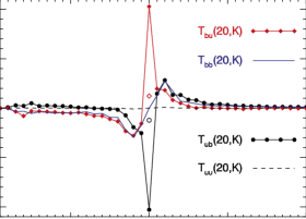
Figure 2: (Color online) Spectral fluxes [Eqs. (6), (9), (7), and (10)] showing incoming and outgoing energy transfers between different shells and fields to/from shell $Q$=20.

$\mathcal{A}_{{}_{ub}}^{(K)}$ is the flux due to the linear terms $\propto\partial_{z}$ in Eqs. (1). It does not transfer energy between different shells, but only in the same shell between fields $\mathbf{u}$ and $\mathbf{b}$. Notice that it has been symmetrized so that $\mathcal{A}_{{}_{ub}}^{(K)}=-\mathcal{A}_{{}_{bu}}^{(K)}$, as can be verified integrating by parts.

Equations (3)-(4) show that at the injection scale (shells 3 and 4) the photospheric forcing supplies energy at the same rate to both kinetic and magnetic energies, i.e., the forcing injects Alfvén waves unlike standard forced MHD turbulence where a mechanical force injects only kinetic energy.

The simulation is started with vanishing orthogonal velocity and magnetic fields ($\mathbf{u}=\mathbf{b}=0$) and a uniform axial magnetic field $\mathbf{B}=B_{0}\,\mathbf{\hat{e}_{z}}$ inside the computational box. As shown in our previous works Rappazzo et al. (2008) the constant forcing velocity at the boundary advects magnetic field lines generating a perpendicular component $\mathbf{b}$. This initially grows linearly in time before saturating nonlinearities develop, and kinetic and magnetic energies then fluctuate around a mean value, with magnetic field fluctuations dominating: $E_{{}_{M}}/E_{{}_{K}}\!\sim 87$ for the simulation presented here.

The magnetic and kinetic energy imbalance is reflected in the energy spectra shown in Fig. 1. Both spectra are peaked at the injection wave numbers 3 and 4, but beyond $n_{{}_{\!\perp}}\!$= 5 an inertial range is resolved where both spectra exhibit a power-law behavior with a steep index for the magnetic energy ($-2.7$) and a flatter one for the kinetic energy ($-0.6$). Since increments are obtained from band-integrated spectra [e.g., $\delta b^{2}(k_{{}_{\!\perp}}\!)\simeq k_{{}_{\!\perp}}E_{M}(k_{{}_{\!\perp}}\!)$], this implies

$$\delta b_{{}_{\!\ell}}\simeq\ell^{\sigma_{{}_{\!b}}},\quad\delta u_{{}_{\!\ell}}\simeq\ell^{\sigma_{{}_{\!u}}},\quad\sigma_{{}_{\!b}}\sim 0.85,\quad\sigma_{{}_{\!u}}\sim-0.2,$$ (12)

i.e., while magnetic energy decreases at small scales kinetic energy increases as it is expected to do for magnetic reconnection Lazarian & Vishniac (1999) where velocity is concentrated at small-scale current sheets Rappazzo et al. (2008).

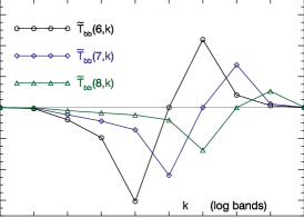
Figure 3: (Color online) Energy flows between scales (log bands) of the magnetic field. Log bands $(p_{k}]$=$(2^{k-2},2^{k-1}]$; see text.

Energy fluxes are shown in Fig. 2. As their behavior is similar along the whole inertial range, here we plot the fluxes in and out of shell $Q=20$. With respect to the equipartition case (EQPT) Alexakis et al. (2005), the most striking difference is the small value of the transfers between kinetic energy shells $\mathcal{T}_{{}_{uu}}^{(Q=20,K)}$, negligible with respect to the others. Indeed, the velocity eddies are not distorted by other velocity eddies as they are too weak compared to the strength of the magnetic field: both the orthogonal component $\mathbf{b}$ and the strong axial field $B_{0}$ are responsible for shaping the velocity field.

We analyze first the energy flows between shells of the magnetic field $\mathcal{T}_{{}_{bb}}^{(Q=20,K)}$. They are negative for all K$<$Q and positive for all K$>$Q meaning that the field is receiving energy from shells at smaller K and giving energy to shells of greater K. In contrast to EQPT for K$<$Q there is an almost constant small contribution from smaller K shells. As in Alexakis et al. (2005) a similar “tail” is also present for $\mathcal{T}_{{}_{bu}}^{(Q=20,K)}$, the magnetic field in shell 20 is receiving energy from smaller K shells of the velocity field and transferring it to larger K shells. $\mathcal{T}_{{}_{ub}}^{(Q=20,K)}=-\mathcal{T}_{{}_{bu}}^{(K,Q=20)}$ has the corresponding behavior.

The large peaks at K=20 represent the conversion of magnetic to kinetic energy in the same shell and are due to $\mathcal{A}_{{}_{bu}}^{(K=20)}\!>0$ ($\mathcal{A}_{{}_{ub}}^{(K)}\!=\!-\mathcal{A}_{{}_{bu}}^{(K)}$). Its large value is linked to the field-line tension of the dominant axial field $B_{0}$ as $\mathcal{A}_{{}_{bu}}$ is obtained from the linear terms $\propto c_{{}_{A}}\partial_{z}$ in eqs. (1), this is the Alfvén propagation term that in presence of a $b_{{}_{\!\perp}}$ contributes with a velocity $u_{{}_{\!\perp}}$ of the same shape. In Fig. 2 the values of the cross-field fluxes $\mathcal{T}_{{}_{bu}}$ and $\mathcal{T}_{{}_{ub}}$ for K=20 without these contributions are shown with a diamond and a solid circle, respectively

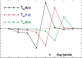
Figure 4: (Color online) Energy fluxes from magnetic to velocity fields scales. Log bands, e.g., $(p_{3}]$=[3, 4] and $(p_{6}]$=[17, 32]

.

The “tails” shown in Fig. 2 are also present for higher values of $Q$. In Alexakis et al. (2005), they were present only in cross-fields transfers, while here a comparable tail appears also in $\mathcal{T}_{{}_{bb}}$. The tail in this work is due to the steeper spectrum of the magnetic field; this induces a higher spectral transfer at low $K$ because of the higher value of $\mathbf{b}_{{}_{K}}$ in flux $\mathcal{T}_{{}_{bb}}$ [Eq. (9)] with respect to the EQPT case Alexakis et al. (2005). This feature has been indicated as evidence of the nonlocal nature of energy transfers in MHD turbulence Alexakis et al. (2005) because the cumulative transfers of farther shells seem to be more important than those of closer shells.

However, in scaling models of MHD turbulence Goldreich and Sridhar (1995); Galtier et al. (2000) and of Parker’s model Rappazzo et al. (2007); *Rappazzo:2008p344; *Rappazzo:2010p4099 scales are defined as log bands of shells. In fact a single shell does not represent a scale since, from the uncertainty principle, its associated field [Eq. (2)] is delocalized in space and cannot represent an eddy, the building block of K41 phenomenology.

Thus in order to understand how energy flows across scales we must use such log bands Aluie and Eyink (2010). Log band $(p]$ is defined as the shells included in $(p/2,p]$, equally spaced on a logarithmic scale. Considering $p_{n}\!=2^{n-1}$ we will indicate these intervals with their index $n$: $(p_{n}]=(2^{n-2},2^{n-1}]$ (n=1,…,10). With a $1024^{2}$ grid we have “only” $10$ distinct intervals. Figures 3 and 4 show the fluxes summed over these log bands of shells, e.g., $\widetilde{T}_{{}_{bb}}^{(q,k)}\!=\!\mathcal{T}_{{}_{bb}}^{(\,(p_{q}],(p_{k}]\,)}$ for q=6, 7 and 8. The injection scale is now $(p_{3}]$=[3,4], while $(p_{6}]$=[17,32], $(p_{7}]$=[33,64], $(p_{8}]$=[65,128], etc..

Figures 3-4 show that the apparently dominating contributions of distant shells (tails in Fig. 2) strongly decrease when considering log bands. In these bands the number of shells increases exponentially at higher wave numbers and the aggregate effect of local transfers asymptotically dominates Aluie and Eyink (2010); Aluie & Eyink (2009). Recently an analytical upper bound has been set for the locality of energy transfers Aluie and Eyink (2010), although within these bounds the energy transfers can be quite spread out Beresnyak & Lazarian (2010). In fact while cross energy transfers (Fig. 4) are quite local as energy flows between neighboring scales decrease swiftly, the transfers between scales of the magnetic field (Fig. 3) are more spread out. However for the Parker problem we do not observe a direct flow of energy between the forcing scale and the small scales Yousef et al. (2007).

Figure 5: Diagram of energy flows between fields and scales.

Overall energy is transferred from larger to smaller scales in a similar fashion as in MHD turbulence with energies in equipartition, except for the velocity field that is too weak compared to the magnetic field. As a result the magnetic field creates and shapes the velocity field. In fact from cross-field flows (Fig. 4) we see that magnetic field line tension enhanced by line tying, and predominantly represented by the fluxes $\mathcal{A}_{{}_{bu}}$, converts magnetic energy to kinetic energy at the same scale. In turn kinetic energy at larger scales is converted to magnetic energy at smaller scales, due to the magnetic stretching term. The magnetic advection term transfers a (smaller) fraction of energy toward smaller magnetic field scales (Fig. 3). A pictorial summary of the cascade is shown in Fig. 5 (magnetic flux spread not shown); the repeated conversion of kinetic to magnetic energies by the cross-field flows effectively cascades energy toward the small scales.

The upper bound for the locality of energy transfers found by Aluie and Eyink (2010) has been restricted to the case $0<\sigma_{{}_{\!b,u}}<1$ in analogy to the hydrodynamic case Aluie & Eyink (2009) but this condition is overrestrictive for MHD and we show that those bounds are valid also for the case [Eq. (12)] where $\sigma_{{}_{\!b}}\sim 0.85$, but $\sigma_{{}_{\!u}}\sim-0.2$ instead of the standard $\sigma_{{}_{\!b,u}}\sim 1/3$.

If $[K]$ is the log band of shells $[K/2,K]$, heuristic scalings [Eq. (12)] can be written more precisely for the generic band-summed field $\mathbf{a}^{[K]}=\sum\mathbf{a}_{{}_{K}}$ with $K\in[K]$ [Eq. (2)] as

$$\langle|\mathbf{a}^{[K]}|^{3}\rangle^{1/3}\simeq K^{-\sigma_{{}_{\!a}}}\quad\rightarrow\quad\langle|\nabla\mathbf{a}^{[K]}|^{3}\rangle^{1/3}\simeq K^{1-\sigma_{{}_{\!a}}}.$$ (13)

Since the scaling for the derivative is valid independently of the sign of $\sigma_{{}_{\!a}}$, following Aluie and Eyink (2010) the bound for the locality of cross-field transfers between band-summed fields is

$$\left|\,T_{{}_{bu}}^{(\,[Q],[K]\,)}\,\right|\leq K^{-(\sigma_{u}+\sigma_{b})}\,Q^{1-\sigma_{b}},\quad\textrm{for}\quad Q\ll K\quad$$ (14)

$$\left|\,T_{{}_{bu}}^{(\,[Q],[K]\,)}\,\right|\leq K^{1-\sigma_{u}}\,Q^{-2\sigma_{b}},\qquad\ \ \textrm{for}\quad Q\gg K$$ (15)

At fixed $K$, contributions from smaller bands [Eq. (14)] are negligible if $\sigma_{{}_{\!b}}<1$ so as from bigger bands [Eq. (15)] for $\sigma_{{}_{\!b}}>0$.

In similar fashion, we obtain the following bound for magnetic fluxes:

$$\left|\,T_{{}_{bb}}^{(\,[Q],[K]\,)}\,\right|\leq K^{-(\sigma_{u}+\sigma_{b})}\,Q^{1-\sigma_{b}},\quad\textrm{for}\quad Q\ll K$$ (16)

$$\left|\,T_{{}_{bb}}^{(\,[Q],[K]\,)}\,\right|\leq K^{1-\sigma_{b}}\,Q^{-(\sigma_{u}+\sigma_{b})},\quad\textrm{for}\quad Q\gg K$$ (17)

The requirement for asymptotic locality is still $\sigma_{{}_{\!b}}<1$ for Eq. (16), but $\sigma_{{}_{\!u}}+\sigma_{{}_{\!b}}>0$ for Eq. (17), all satisfied in our case.

The sign of the exponents containing $\sigma_{{}_{\!u}}$ remains unaltered with respect to the classic case $\sigma_{{}_{\!b,u}}\sim 1/3$, but while in Eqs. (14) and (16) $K^{-0.65}$ decreases for large $K$ in Eqs. (15) and (17) we have a positive power ($K^{1.2}$ and $K^{0.15}$, respectively) as in the standard case Aluie and Eyink (2010) with $K^{2/3}$. As in the hydrodynamic case Aluie & Eyink (2009) the origin of this pathological behavior stems from the use of Hölder inequality for fluxes [Eqs. (6)-(9)] to set the upper bound, since only the absolute values of their terms are considered, and any cancellation effect due to the scalar products in Eqs. (6)-(9) is neglected. This conclusion is reinforced by the fact that for Parker problem fluxes, Eqs. (6)-(9) exhibit scalings (not shown) in $Q$ well below upper bounds [Eqs. (14)-(17)].