Casimir-Foucault interaction: Free energy and entropy at low temperature

Abstract

It was recently found that thermodynamic anomalies which arise in the Casimir effect between metals described by the Drude model can be attributed to the interaction of fluctuating Foucault (or eddy) currents [Phys. Rev.  Lett. 103, 130405 (2009)]. We show explicitly that the two leading terms of the low-temperature correction to the Casimir free energy of interaction between two plates, are identical to those pertaining to the Foucault current interaction alone, up to a correction which is very small for good metals. Moreover, a mode density along real frequencies is introduced, showing that the Casimir free energy, as given by the Lifshitz theory, separates in a natural manner in contributions from eddy currents and propagating cavity modes, respectively. The latter have long been known to be of little importance to the low-temperature Casimir anomalies. This convincingly demonstrates that eddy current modes are responsible for the large temperature correction to the Casimir effect between Drude metals, predicted by the Lifshitz theory, but not observed in experiments.

I Introduction

For a decade the finite-temperature correction to the Casimir forceCasimir (1948) between parallel metal plates has been a topic of intense investigation and debate. Describing the metals by a standard Drude model

$$\varepsilon(\omega)=1-\frac{\Omega^{2}}{\omega(\omega+{\rm i}\gamma)},$$ (1)

where $\Omega$ is the plasma frequency and where the relaxation frequency $\gamma$ does not vanish at $T=0$, the Lifshitz theory implies that the temperature dependence is considerably different from perfect reflectorsBoström and Sernelius (2000): a significant thermal contribution is predicted already at distances shorter than the Wien wavelength $\hbar c/(2\pi k_{B}T)$, on the one hand, and there is a difference of a factor $\frac{1}{2}$ in the large-distance limit, on the other. Puzzlingly, such a large temperature dependence is not found in recent precision experiments at Purdue Decca et al. (2007). For reviews of the thermal debate around the Casimir effect, cf. Brevik et al. (2006); Bordag et al. (2009) and references therein.

The thermodynamics of the Casimir effect has been of particular interest in this context. For metals described by (1), the Gibbs-Helmholtz free energy of the Casimir interaction is non-monotonous as a function of temperature, leading to a negative Casimir entropy in a large temperature range Brevik et al. (2006). Moreover, if $\gamma$ vanishes faster than linear as the temperature $T\to 0$, the Casimir entropy remains nonzero in this limit; this was argued to violate Nernst’s theorem, the third law of thermodynamics Klimchitskaya and Mostepanenko (2001).

Recently two of the present authors investigated the contribution to the Casimir force from Johnson-Nyquist noise, focusing on specific solutions of the Maxwell equations for the two-plate set-up, namely purely dissipative (i.e., overdamped) modes which are physically Foucault current or ‘eddy current’ modes Intravaia and Henkel (2009). [A related investigation with a simplified model is due to Bimonte Bimonte (2007).] It was shown that the eddy current contribution alone accounts for the apparently anomalous thermodynamics of the Casimir effect. The non-vanishing entropy that appears when first $\gamma\to 0$ and then $T\to 0$ (taken in this order), is due to an infinite degeneracy of quasi-static Foucault current states, a glass-like situation for which the Nernst theorem does not apply Intravaia and Henkel (2010). The situation is closely analogous to that of a free particle coupled to a heat bath Ingold et al. (2009), which is essentially in its high temperature limit for any nonzero temperature when no damping is present, and for which the Nernst theorem is satisfied for a fixed friction rate Hänggi and Ingold (2006). The apparent thermodynamical anomaly in the Casimir context was investigated in detail in Refs. Intravaia and Henkel (2008); Ellingsen (2008); Ellingsen et al. (2009). It is now established that the Lifshitz theory gives a low-temperature expansion of the Casimir free energy between two Drude metals in the form Ingold et al. (2009); Brevik et al. (2004); Høye et al. (2007); Ellingsen et al. (2008); Brevik et al. (2008); Ellingsen et al. (2009)

$$\Delta F_{\text{CL}}(T)=f_{\text{CL}}^{(2)}T^{2}+f_{\text{CL}}^{(5/2)}T^{5/2}+...$$ (2)

where the free energies are split into

$$F(T)=F_{0}+\Delta F(T),$$ (3)

$F_{0}$ being the zero temperature value. The derivation of these results in Refs.Høye et al. (2007); Brevik et al. (2008); Ellingsen et al. (2008), starting from a Matsubara sum, is quite tricky, see Sec. 3 of Ref. Ellingsen et al. (2009). They were confirmed independently using a scattering approach by Ingold and collaborators Ingold et al. (2009).

In this paper we go one step further in showing how the behavior of the Casimir effect between good Drude metals is dictated entirely by the contribution from Foucault current modes. We introduce a free energy of interaction between Foucault current modes in two Drude plates, and find it to have the same form at low temperatures:

$$\Delta F_{D}(T)=f_{D}^{(2)}T^{2}+f_{D}^{(5/2)}T^{5/2}+...$$ (4)

We use throughout the subscript $D$ to denote the eddy current (or diffusive modes) contribution to the Casimir interaction. We are able to calculate the coefficients $f_{D}^{(2)}$ and $f_{D}^{(5/2)}$ and, quite remarkably, find

$$f_{D}^{(2)} =f_{\text{CL}}^{(2)}+\mathcal{O}[(\gamma/\Omega)^{2}];$$ (5a)

$$f_{D}^{(5/2)} =f_{\text{CL}}^{(5/2)}.$$ (5b)

The calculations are based on an analysis of the zeros and branch cuts of the dispersion function for the Casimir energy, similar to previous work based on the argument principle Davies (1972); Schram (1973). This analysis permits us to identify a density of states (DOS) for both the Foucault-current interaction and the full electromagnetic Casimir interaction within the Lifshitz theory. This method reveals a close relationship between the two interactions, and yields the results (5) in a fairly simple way, including the correction term to $f^{(2)}$ of order $\gamma^{2}/\Omega^{2}$ which we calculate in the limit of good conductors.

The low-temperature expansion is valid on a temperature scale lower than

$$k_{B}T\ll\frac{\hbar D}{L^{2}}=\frac{\hbar\gamma c^{2}}{\Omega^{2}L^{2}}$$ (6)

where $D$ is the diffusion coefficient of Foucault currents Jackson (1975) and $L$ the distance between the plates. This scale (‘Thouless energy’ Thouless (1977)) has been identified in previous work Torgerson and Lamoreaux (2004); Svetovoy (2007); Ellingsen (2008) and emerges naturally when spatially diffusive modes in two half-spaces are coupled by electromagnetic fields across a gap of width $L$ Intravaia and Henkel (2009). It corresponds to a temperature around 20 K for $L=100\,{\rm nm}$ and the conductivity of gold at room temperature. We shall refer frequently to this parameter in the following.

The paper is structured as follows: in section II, we introduce a general scheme for calculating the low temperature expansion of the Gibbs-Helmholtz free energy from DOS functions, and recapitulate the DOS for the Casimir-Lifshitz and Foucault current interactions, respectively. We use a method of contour integration to derive a relation between the DOS of the two types of interaction. This provides an intuitive tool for calculating the desired expansion coefficients $f^{(2)}$ and $f^{(5/2)}$ in section III, first to leading order in the small parameter $\gamma/\Omega$, then the correction term. Various mathematical results are collected in the appendixes.

Throughout the calculation we assume the material be described by (1), and let $\hbar=k_{\rm B}=1$. We shall use the terms eddy current and Foucault current interchangably.

II Mode densities

II.1 Introduction

The Gibbs-Helmholtz free energy $F$ for a system with a continuous distribution of bosonic normal modes is related to the DOS $\rho(\omega)$ (modes per angular frequency) by the relation

$$\Delta F(T) =T\int\limits_{0}^{\infty}\!{\rm d}\omega\,\rho(\omega)\log(1-{\rm e}^{-\omega/T})$$

$$=\int\limits_{0}^{\infty}\!{\rm d}\omega\frac{\mathcal{M}(\omega)}{{\rm e}^{\omega/T}-1},$$ (7)

where $\mathcal{M}(\omega)$ is the integrated mode density:

$$\rho(\omega)=-\partial_{\omega}\mathcal{M}(\omega).$$ (8)

(We fix the integration constant with $\mathcal{M}(0)=0.$) The mode density $\rho(\omega)$ (per angular frequency) specifies the physical system. (Note the difference to the density of states per unit energy introduced in Ref.Hanke and Zwerger (1995).) In the low-temperature limit, the exponential confines the integrand to small values of $\omega$, and we can expand $\mathcal{M}(\omega)$ in powers of $\omega$ [see also Ref. Ford and O’Connell (2005)]. Integrating termwise, each power $\omega^{\nu}$ of the expansion yields a contribution $\sim T^{\nu+1}$ according to

$$\int_{0}^{\infty} \frac{\mathrm{d}\omega\,\omega^{\nu}}{e^{\omega/T}-1}=\Gamma(\nu+1)\zeta(\nu+1)T^{\nu+1}.$$ (9)

This method is the real-frequency analog of the method laid out in Ellingsen et al. (2009) and used in Ellingsen et al. (2008) where Matsubara sums were expanded at low temperatures. The exponential cutoff from the temperature dependence makes the procedure considerably more straightforward here, since standard methods of asymptotic expansion are applicable.

For the two-plate geometry, $F$ is a free energy per area and also depends on their separation $L$, with the corresponding pressure given by $p=-\partial F/\partial L$. The low-frequency expansion of the mode density ${\cal M}_{D}(\omega)$ for diffusive modes is found to be of the form

$$\mathcal{M}_{D}(\omega)\approx\left[m^{(1)}_{D}\frac{\omega}{D}+m^{(3/2)}_{D}L\left(\frac{\omega}{D}\right)^{3/2}\dots\right]$$ (10)

where the inverse diffusion constant $1/D$ conveniently provides the physical units, and the Thouless frequency $D/L^{2}$ gives the relevant frequency scale. The coefficients $m^{(1)}_{D}$, $m^{(3/2)}_{D}$ are dimensionless, the first of which relates quite obviously to the static value of the mode density [see (8)]:

$$\rho_{D}(0)=-\frac{m^{(1)}_{D}}{D}.$$ (11)

Applying the identities (9), we get the desired free energy expansion

$$\Delta F_{D}(T)=\zeta(2)\frac{m^{(1)}_{D}}{D}T^{2}\\ +\frac{\sqrt{\pi}\,\zeta(\frac{5}{2})}{2}m^{(3/2)}_{D}\frac{T^{5/2}L}{D^{3/2}}+\mathcal{O}(T^{3})$$ (12)

where $\zeta(2)=\pi^{2}/6$ and $\zeta(\frac{5}{2})\approx 1.34149$. As we calculate in Section III below

$$m^{(1)}_{D} \approx \frac{2\log 2-1}{8\pi^{2}}+\frac{\lambda(\gamma/\Omega)^{2}}{4\pi^{2}(L+2\lambda)};$$ (13a)

$$m^{(3/2)}_{D} = -\frac{\sqrt{2}}{24\pi^{2}},$$ (13b)

where an expansion for good conductors ($\gamma\ll\Omega$) has been performed, with corrections to $m^{(1)}_{D}$ appearing at the order $\mathcal{O}^{2}(\gamma/\Omega)$. The plasma penetration depth is defined as $\lambda=c/\Omega$. Note that the limit $L\to\infty$ cannot be applied here, since it conflicts with the small parameter $TL^{2}/D$ in the expansion [Eq.(6)]; this is why the scaling with $L$ in the third term on the right hand side of of Eq.(12) is not unphysical. In the limit $L\to 0$, $\Delta F_{D}$ is nonzero and finite: this can be attributed to the change in the bulk self-energy of the electromagnetic excitations of the metallic medium, as a pair of surfaces is introduced (the ‘cleavage energy’ discussed by Barton Barton (1979)). The surfaces introduce boundary conditions for the fluctuating electromagnetic modes (eddy currents in this case), leading to a change in energy per area with respect to a uniform bulk medium.

We identify in the two following Sections the mode densities $\rho_{\rm CL}(\omega)$ and $\rho_{D}(\omega)$ that determine, respectively, the free energy due to all modes and due to diffusive modes. The former quantity is calculated within the Lifshitz theory for the Casimir effectLifshitz (1956).

II.2 All modes: Lifshitz mode density

Let us recall that the mode density $\rho_{\rm CL}(\omega)$ counts how the mode number at a given frequency $\omega$ for two half-spaces at separation $L$ differs from the situation of two plates at infinite distance. The Lifshitz formula for the Casimir free energy Parsegian (2006) can be written in the form of Eq.(7) so that the following form of the mode density can be read off

$$\rho_{\text{CL}}(\omega)=-{\rm Im}\,\partial_{\omega}\mathcal{D}(z=\omega+{\rm i}0).$$ (14)

Here and henceforth, let $z$ denote a complex frequency. The “dispersion function” $\mathcal{D}(z)$ is given by the integral

$$\mathcal{D}(z)\equiv \sum_{\sigma=\mathrm{p},\mathrm{s}}\mathcal{D}^{\sigma}$$

$$= \sum_{\sigma=\mathrm{p},\mathrm{s}}\int\limits_{0}^{\infty}\!\frac{k{\rm d}k}{2\pi^{2}}\log\left[1-r_{\sigma}^{2}(\kappa,z)\,{\rm e}^{-2\kappa L}\right],$$ (15)

Here, $\kappa=\sqrt{{k}^{2}-z^{2}/c^{2}}$, $\sigma$ is a polarization index, and $L$ the cavity width. In the following, we only consider the s- (or TE-) polarization and drop the polarization label. The reflection coefficient becomes (using the Drude dielectric function (1))

$$r(\kappa,z) = r_{\rm s}(\kappa,z)=\frac{\kappa-\sqrt{\kappa^{2}+\kappa_{\gamma}^{2}(z)}}{\kappa+\sqrt{\kappa^{2}+\kappa_{\gamma}^{2}(z)}};$$ (16a)

$$\kappa_{\gamma}(z) = \frac{\Omega}{c}\sqrt{\frac{z}{z+{\rm i}\gamma}}.$$ (16b)

All square roots are chosen here with positive real part; this implies in particular that ${\rm Im}\,\kappa\leq 0$ and ${\rm Im}\sqrt{\kappa^{2}+\kappa_{\gamma}^{2}(z)}\leq 0$ for $z$ in the upper half-plane.

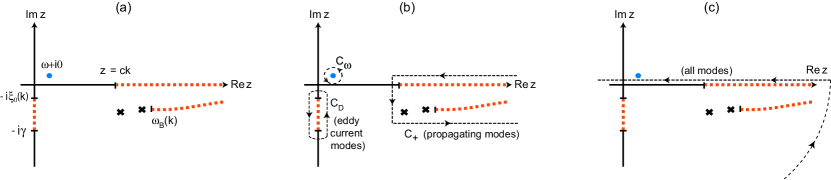
Figure 1: (Color online) (a) Complex eigenfrequencies in the parallel plate geometry, for a fixed wavevector $k$ (not to scale). The thick dotted lines show branch cuts (three-dimensional mode continuum), crosses mark poles (discrete frequencies). The circular dot is a pole of the first factor in Eq.(24). The pole structure is symmetric with respect to the imaginary axis, according to Eq.(25). The frequency $\omega_{\mathrm{B}}(k)$ marks the transition from discrete cavity modes to a continuum of bulk modes (see Intravaia et al. (2007) for details). (b) Integration path: $C_{D}$ around the eddy current continuum, $C_{\omega}$ around the pole at $z=\omega+{\rm i}0$, $C_{+}$ around cavity and propagating modes. The corresponding paths in the left half-plane are denoted $C_{-\omega}$ and $C_{-}$, respectively. (c) Integration path that encircles all modes, as relevant for the Lifshitz theory. Closing this contour in the upper half-plane, one gets the residue from the pole $z=\omega+{\rm i}0$ in the upper half-plane.

II.3 Eddy current modes

The dispersion function $\mathcal{D}(z)$ is analytic in the upper half-plane. When it is analytically continued, singularities appear on the real axis and in the lower half-plane: branch points where the argument of the logarithm in Eq.(15) vanishes, and branch cuts from the square roots involved in the reflection coefficients (see Fig.1). These singularities are related to the electromagnetic resonance frequencies of the two-plate setup that determine the Lifshitz free energy from the argument principle Schram (1973); Intravaia and Henkel (2008, 2010). They also provide a physically well-motivated way to isolate the contribution of a particular class of modes to the Casimir interaction.

The eddy current (diffusive) modes, for fixed $k$, are identified as a branch cut of $\mathcal{D}(z)$ along the negative imaginary frequency axis (see figure 1), $z=-i\xi_{0}\ldots-{\rm i}\gamma$ ($\xi_{0}=\xi_{0}(k)$ is defined below). This branch cut is an example of a dispersion function that is not real on the imaginary frequency axis, in distinction to the familiar behavior in the upper half-plane. Indeed, one can confirm from the macroscopic Maxwell equations that purely imaginary eigenfrequencies appear in a planar cavity of two half-spaces described by the Drude dielectric function Jackson (1975). As is well-known in scattering theory (see, e.g. Ref.Schram (1973); Nesterenko (2006)), the branch cut can be interpreted as a dense coalescence of discrete modes, and the relevant quantity is a mode density given by

$$\mu_{D}(\xi)=-{\rm Im}\,\partial_{\xi}\mathcal{D}(z=-{\rm i}\xi+0),\quad 0\leq\xi\leq\gamma.$$ (17)

The dispersion function is evaluated here to the right of the branch cut. Continuing analytically from the upper half-plane, we find that $\kappa$ is mainly real, while $\kappa_{\gamma}(-{\rm i}\xi+0)=-{\rm i}k_{\gamma}(\xi)$ becomes mainly imaginary with

$$k_{\gamma}(\xi)=\frac{\Omega}{c}\sqrt{\frac{\xi}{\gamma-\xi}}.$$ (18)

As a consequence, $[\kappa^{2}-k_{\gamma}^{2}(\xi)]^{1/2}$ moves to the (negative) imaginary axis if $\kappa$ is small enough; more precisely, we require

$$0\leq\kappa\leq k_{\gamma}(\xi)$$ (19)

This is equivalent to

$$\xi_{0}(k)\leq\xi\leq\gamma$$ (20)

where the lower bound $\xi_{0}(k)$ solves

$$(\gamma-\xi_{0})(c^{2}k^{2}+\xi_{0}^{2})=\Omega^{2}\xi_{0}.$$ (21)

We note the limiting behavior $\xi_{0}(k)\approx Dk^{2}$ as $k\to 0$ where $D$ is the diffusion coefficient of Eq.(6). In the range (20), the reflection coefficient becomes the unitary number

$$r(\kappa,-{\rm i}\xi+0)=\frac{\kappa+{\rm i}\sqrt{k_{\gamma}^{2}(\xi)-\kappa^{2}}}{\kappa-{\rm i}\sqrt{k_{\gamma}^{2}(\xi)-\kappa^{2}}}$$ (22)

where the sign of the square root applies on the right side of the branch cut and follows by carefully evaluating the imaginary parts of $\kappa$ and $k_{\gamma}(\xi)$. For imaginary frequencies outside the range (20), the reflection coefficient is real ($-1<r_{\rm s}<0$), and the eddy current mode density (17) vanishes.

After integrating over $k$, one gets a mode density $\mu_{D}(\xi)$ that is nonzero in the range $0\leq\xi\leq\gamma$. Finally, the density for eddy current modes $\rho_{D}(\omega)$ at real frequencies is defined by associating to each overdamped mode $z=-{\rm i}\xi$ a Lorentzian spectrum centered at zero frequency whose width is $\sim{\rm Im}\,z$. Referring to Ref.Intravaia and Henkel (2009) for details, we get

$$\rho_{D}(\omega) =\int\limits_{0}^{\gamma}\frac{\mathrm{d}\xi}{\pi}\frac{\xi}{\xi^{2}+\omega^{2}}\mu_{D}(\xi).$$ (23)

II.4 Contour integral representation

In this section we derive a contour integral represention for the mode densities of the full Casimir-Lifshitz interaction and of the eddy current contribution. This demonstrates a simple relation between $\rho_{\text{CL}}(\omega)$ and $\rho_{D}(\omega)$. We thus prepare the low-frequency analysis we perform in Sec.III focusing on the particular case of a good Drude conductor (i.e., $\gamma\ll\Omega$).

It is easy to see from the sign flip of the root involving $\kappa_{\gamma}(\xi)$ in Eq.(16), that the dispersion function $\mathcal{D}(z)$ jumps and changes into its complex conjugate across the branch cut $z=0\ldots-{\rm i}\gamma$. This jump defines the eddy current DOS in Eq.(17). The latter can thus be written as a contour integral in the complex plane,

$$\rho_{D}(\omega)=-\,\oint\limits_{C_{D}}\frac{\mathrm{d}z}{2\pi}\frac{z}{z^{2}-\omega^{2}}\partial_{z}\mathcal{D}(z),$$ (24)

where the path $C_{D}$ encircles the cut on the negative imaginary axis in the positive sense as shown in Fig.1(b). Now, shifting the contour towards infinity, we encounter the poles at $z=\pm\omega$ from Eq.(24) and other singularities (poles and branch cuts) of $\partial_{z}\mathcal{D}(z)$. The behavior of the exponential ${\rm e}^{-2\kappa L}$ for $|z|\to\infty$ makes $\mathcal{D}(z)$ vanish at infinity. Hence we conclude that the integral around $C_{D}$ is equal to the negative residues of the poles $z=\pm\omega$ minus integrals over the contours $C_{\pm}$ in Fig.1(b) that encircle the singularities near the left and right half of the real axis. We use here the link between the dispersion function and the response (or Green) function of the two-plate cavity Davies (1972); Schram (1973) that entails the symmetry relation

$$\mathcal{D}(-z^{*})=\mathcal{D}^{*}(z)\;.$$ (25)

As a consequence, complex mode frequencies and branch cuts appear in pairs on opposite sides of the imaginary axis. (In Fig.1, only the right half is shown.)

The residues at the poles are easily calculated from the contours $C_{\pm\omega}$ in Fig.1(b):

$$\oint\limits_{C_{\omega}+C_{-\omega}}\frac{{\rm d}z}{2\pi} \frac{z}{z^{2}-\omega^{2}}\partial_{z}\mathcal{D}(z)=\frac{{\rm i}}{2}\left(\partial_{z}\mathcal{D}(\omega)+\partial_{z}\mathcal{D}(-\omega)\right)$$

$$=-{\rm Im}\partial_{\omega}\mathcal{D}(\omega)=\rho_{\text{CL}}(\omega)$$ (26)

We thus recover the mode density for the Lifshitz theory as one term in the eddy current DOS. This is actually not surprising, since $\rho_{\text{CL}}(\omega)$ can be written as a similar contour integral as Eq.(24), but evaluated along a contour just above the real axis [Fig.1(c)] and closed at infinity in the lower half plane. This contour encircles all singularities of the dispersion function as it should, since the Lifshitz theory accounts for all modes. If this contour is shifted through infinity into the upper half-plane, only the two residues calculated in Eq.(26) contribute since the dispersion function is analytic inside the contour.

In conclusion, we can write the following splitting of the mode density for the Casimir effect

$$\rho_{\text{CL}}(\omega)=\rho_{D}(\omega)+\rho_{\pm}(\omega)$$ (27)

where the last term gives the contribution of modes near the real axis (contour $C_{+}$ in Fig.1(b), and corresponding $C_{-}$ in the left half-plane). By continuity with the limiting case $\gamma\to 0$, we can identify the latter modes with propagating modes in the vacuum cavity, in the bulk, or with electromagnetic surface modes (for example, surface plasmons that appear in the TM-polarization). We shall see in the next section that for nonzero, but small $\gamma\ll\Omega$, the mode density $\rho_{\pm}(\omega)$ becomes small at low frequencies ($\omega<D/L^{2},\gamma,c/L$), so that in this range, the full electromagnetic DOS $\rho_{\text{CL}}(\omega)$ nearly coincides with the eddy current DOS $\rho_{D}(\omega)$.

III Low-frequency expansion

We calculate now the small $\omega$ expansion of the density of states for eddy current modes. According to Eq. (27), we start with the full Casimir-Lifshitz interaction and discuss then the differences between the two. We begin with a general estimate of the scaling for good conductors.

III.1 Scaling for weak damping

The analysis in the complex plane, as illustrated in Fig.1, suggests that the density of diffusive modes is concentrated in a range $\sim\gamma$ near zero frequency. Anticipating from the analysis below a total number of $\sim 1/L^{2}$ modes per unit area, one gets for $\gamma\to 0$ a scaling $\rho_{D}(\omega)\approx 1/(\gamma L^{2})\theta(\omega/\gamma,L/\lambda)$ where the frequency appears in the function $\theta$ only in the dimensionless form $\omega/\gamma$ (and similarly for the distance $L/\lambda\equiv\Omega L/c$). A different behavior emerges for propagating modes (inside the contour $C_{+}$ in Fig.1): they move onto the real axis for small $\gamma$ and contribute to $\rho_{\pm}(\omega)$ in the range $\omega\sim c/L,\Omega$. Their contribution at much lower frequencies that interests us here, is proportional to their imaginary part and therefore scales linearly with $\gamma$. This observation shall provide us with a simple rule to identify the respective contributions of eddy current and propagating modes in the full (Lifshitz) mode density, Sec.III.2. Note that we consider here the case of a fixed (temperature-independent) scattering rate $\gamma$.

Some further corroboration of these rough estimates is desirable. Let us consider for the simplicity of argument that the dispersion function $\partial_{z}\mathcal{D}(z)$ has only discrete poles $\omega_{n}(k)$ in the lower half-plane, labelled by the momentum quantum number $k$. This can be achieved by enclosing the system in a finite box Schram (1973); Intravaia and Henkel (2008). One recovers the branch cuts by taking the box size to infinity Nesterenko (2006). From the symmetry relation (25), the poles occur either on the imaginary axis (as for diffusive modes) or pairwise in the lower left and right quadrants (as for propagating modes). The two terms $\rho_{D}(\omega)$ and $\rho_{\pm}(\omega)$ collect these poles, respectively.

We make the replacement ${\rm d}\xi\,\mu_{D}(\xi)\mapsto{\rm d}^{2}k/(2\pi)^{2}\sum_{n\in\text{eddy}}$ and find that the DOS for diffusive modes $\rho_{D}(\omega)$ can be written in the following scaling form

$$\rho_{D}(\omega)=\frac{1}{\gamma}\int\!\frac{k{\rm d}k}{2\pi^{2}}\,\bigg{[}\sum_{n\in\text{eddy}}\frac{\xi_{n}(k)/\gamma}{(\omega/\gamma)^{2}+(\xi_{n}(k)/\gamma)^{2}}\bigg{]}^{L}_{L\to\infty}\\$$

where the limit of the mode branches for two separate plates ($L\to\infty$) is subtracted. We have already seen that the mode frequencies satisfy $\xi_{n}(k)\leq\gamma$. As a consequence, the integral tends toward a finite limit as $\gamma\to 0$, $\rho_{D}(\omega)$ depends only on the scaled frequency $\omega/\gamma$ and is proportional to the scaling factor $1/\gamma$. This implies in particular that the integral over the diffusive mode density can give a nonzero contribution even as $\gamma\to 0$. We confirm these results in Eq.(36) below.

The density of propagating modes $\rho_{\pm}(\omega)$ shows a different scaling with $\gamma$. With the same re-writing, the contours $C_{+}$ and $C_{-}$ collect the modes away from the imaginary axis and lead to the representation

$$\rho_{\pm}(\omega) =-\oint_{C_{+}+C_{-}}\!\frac{{\rm d}z}{2\pi}\frac{z}{z^{2}-\omega^{2}}\partial_{z}\mathcal{D}(z)$$

$$=-\int_{0}^{\infty}\!\frac{k{\rm d}k}{2\pi^{2}}\,{\rm Im}\bigg{[}\sum_{n\in\text{prop}}\frac{\omega_{n}(k)}{\omega^{2}-\omega^{2}_{n}(k)}\bigg{]}^{L}_{L\to\infty}$$ (28)

where in the second line, we represent the modes by the poles in the lower right quadrant. Now, the imaginary part of the eigenfrequency $\omega_{n}(k)$ is negative and, for a small Drude scattering rate, of the order $\gamma$. A typical scale for its real part, on the other hand, is the lowest cavity eigenfrequency $c/L$ or the plasma frequency $\Omega$. Although we do not need them here, recall that the surface plasmon modes appear at $\approx\Omega/\sqrt{2}-{\rm i}\gamma/2$ for $k\gg\Omega/c$ Raether (1988). For an estimate of $\rho_{\pm}(\omega)$, we focus on frequencies $\omega$ much smaller than the real part, $\omega\ll c/L,\Omega$ and take $1/L$ to estimate the relevant wave vectors. This gives

$$\omega\to 0:\quad\rho_{\pm}(\omega)\sim\mathcal{O}\big{(}\frac{\gamma}{\Omega^{2}L^{2}}\big{)}\ldots\mathcal{O}\big{(}\frac{\gamma}{c^{2}}\big{)}$$ (29)

as we confirm in Eq.(44) below. This small “tail” of the mode density near zero frequency can be understood from the broadening of the discrete modes due to damping (a $\delta$-peak becomes similar to a Lorentzian, see also Ref.Hanke and Zwerger (1995)). In particular, it vanishes in the limit $\gamma\to 0$ where $\rho_{\pm}(\omega)$ goes over into the mode density of the plasma model which scales proportional to $\omega^{2}$.

To summarize this estimate, we expect from Eq.(27) that as $\gamma\to 0$, the low-frequency mode density for the Casimir-Foucault interaction and for the full Casimir interaction coincide in order $1/\gamma$, with a small difference $\sim\gamma$ arising from propagating modes. These contributions are calculated in the following sections. We are thus able to check our approach against the free energy expansion of Refs.Høye et al. (2007); Ellingsen et al. (2008).

III.2 Lowest order: Lifshitz theory

Let us calculate the coefficients $m^{(1)}_{D}$ and $m^{(3/2)}_{D}$ defined in Eq. (10), starting with the leading order in the small parameter $\gamma/\Omega$ which, as we have just seen, is provided by the full Lifshitz theory. It is convenient to work with the integrated mode density which from Eq.(14), we can read off as

$$\mathcal{M}_{\rm CL}(\omega)={\rm Im}\,\mathcal{D}(\omega+{\rm i}0).$$ (30)

We therefore start by analyzing in detail the behavior of $\mathcal{D}(z)$ for small frequencies $|z|\ll\gamma$.

The $k$-integral in Eq.(15) is re-written in terms of a real variable $y>0$ defined by $\kappa=y\kappa_{\gamma}(z)$. This is equivalent to a shift of the integration path in the complex $\kappa$-plane along a more convenient direction: one still has convergence from the exponential $\exp(-2\kappa L)$ because ${\rm Re}\,\kappa_{\gamma}(z)>0$ (keeping clear of the branch cut for $z$ on the negative imaginary axis). The reflection coefficient (16) becomes real along this direction and independent of $z$:

$$r(y)=\frac{y-\sqrt{y^{2}+1}}{y+\sqrt{y^{2}+1}}=\frac{1}{(y+\sqrt{y^{2}+1})^{2}}.$$ (31)

We get

$$\mathcal{D}(z)=\kappa^{2}_{\gamma}(z)\int\limits_{\chi(z)}^{\infty}\frac{y\mathrm{d}y}{2\pi^{2}}\log\left[1-r^{2}(y)e^{-2y\kappa_{\gamma}(z)L}\right]$$ (32)

where the lower limit is given by the complex number

$$\chi(z)=-\frac{\mathrm{i}z}{c\kappa_{\gamma}(z)}=-\frac{{\rm i}z}{\Omega}\sqrt{\frac{z+{\rm i}\gamma}{z}}.$$ (33)

For $|z|<\gamma$, we have $|\chi(z)|\leq\sqrt{2}(\gamma/\Omega)\ll 1$ for a good conductor, and to leading order, we can replace the lower limit in Eq.(32) by zero. This defines $\mathcal{D}_{0}(z)$ and via Eq.(30), $\mathcal{M}_{{\rm CL},0}(\omega)$. We write $\mathcal{M}_{{\rm CL},\gamma}(\omega)$ for the error (i.e., the integral from $0$ to $\chi(z)$) and calculate it in Eq.(37) below.

By inspection, $\mathcal{D}_{0}(z)$ depends on $z$ only via the function $\kappa_{\gamma}(z)$ that can be written as

$$\kappa_{\gamma}(z)=\kappa_{1}(z/\gamma)=\frac{\Omega}{c}\sqrt{\frac{z/\gamma}{z/\gamma+\mathrm{i}}},$$ (34)

involving the scaled quantity $z/\gamma$. From the reflection coefficient $r(y)$, the relevant integration domain is $0\leq y\lesssim 1$. We can therefore expand the exponential in Eq.(32) provided $\kappa_{1}(z/\gamma)L\ll 1$. This yields the condition $(|z|/\xi_{L})^{1/2}\ll 1$ where $\xi_{L}$ is the Thouless frequency introduced in Eq.(6). Expanding to the first order in this small parameter, we get ($D$ is the diffusion coefficient)

$$\mathcal{D}_{0}(z) \approx\frac{z}{{\rm i}D}\int\limits_{0}^{\infty}\frac{y\mathrm{d}y}{2\pi^{2}}\log\left[1-r^{2}(y)\right]$$ (35)

$${}+\frac{z}{{\rm i}D}\Big{(}\frac{z}{{\rm i}\xi_{L}}\Big{)}^{1/2}\int\limits_{0}^{\infty}\!\frac{y^{2}\mathrm{d}y}{2\pi^{2}}\frac{2r^{2}(y)}{1-r^{2}(y)}+\mathcal{O}^{2}(z/\xi_{L})$$

where powers $z$ and $z^{3/2}$ have appeared. The integrals can be solved exactly (see Appendix A), and we get from Eq.(30) the following approximation to the Lifshitz integrated DOS

$$\mathcal{M}_{{\rm CL},0}(\omega)\approx\frac{2\log 2-1}{8\pi^{2}}\frac{\omega}{D}-\frac{L\sqrt{2}}{24\pi^{2}}\left(\frac{\omega}{D}\right)^{3/2}$$ (36)

valid for $\omega\ll\xi_{L},\gamma$. This proves the first term in Eqs.(13). It is clear from this calculation (a power series in $(\omega/\xi_{L})^{1/2}$) that these results cannot be applied for $\gamma\to 0$ at fixed $\omega>0$. In other words, the limits $\gamma\to 0$ and $\omega\to 0$ do not commute. For a discussion, see Refs. Intravaia and Henkel (2008); Ellingsen (2008).

Calculate now the small correction $\mathcal{M}_{{\rm CL},\gamma}(\omega)$ from the lower integration limit in Eq.(32). This arises between the boundaries $y=0$ and $y=\chi(z)$. Recall that in the limit $\gamma\ll\Omega$, we have $|\chi(z)|\ll 1$ and expand the integrand for $y\ll 1$. This gives

$$\mathcal{M}_{{\rm CL},\gamma}(\omega) \approx-{\rm Im}\,\kappa^{2}_{\gamma}(z)\!\!\int\limits_{0}^{\chi(z)}\frac{y\mathrm{d}y}{2\pi^{2}}\log\left[2y(2+\kappa_{\gamma}(z)L)\right]$$

$$\approx-\frac{1}{16\pi}\frac{\omega^{2}}{c^{2}},$$ (37)

one half the mode density for the so-called plasma model where $\gamma=0$ is taken from the outset. Notably, this term gives a contribution to the free energy proportional to $T^{3}$, which exactly coincides with the expression given in Ellingsen et al. (2008, 2009). Note that the term scaling with Eq.(29) has not appeared in the full (Lifshitz) mode density. We outline an interpretation in Sec.IV.

III.3 Eddy current modes

We now address the density of eddy current modes alone that involves according to Eq.(23) an integral along the branch cut of $\mathcal{D}(z)$ on the imaginary axis. It is again convenient to work out the integrated mode density ${\cal M}_{D}(\omega)$. A partial integration leads to the integral representation

$$\mathcal{M}_{D}(\omega)=-\int\limits_{0}^{\gamma}\frac{\mathrm{d}\xi}{\pi}\frac{\omega}{\xi^{2}+\omega^{2}}M_{D}(\xi).$$ (38)

where $M_{D}(\xi)$ is the integrated mode density along the branch cut. By changing the momentum variable from $k$ to $\kappa$, this function can be written as

$$M_{D}(\xi)=-\int\limits_{\xi/c}^{k_{\gamma}(\xi)}\frac{\kappa\mathrm{d}\kappa}{2\pi^{2}}{\rm Im}\log[1-r^{2}(\kappa,-{\rm i}\xi)e^{-2\kappa L}],$$ (39)

where the integrand is zero above the upper integration limit $k_{\gamma}(\xi)$ that was defined in (18).

The limiting behavior of this expression for a good conductor can be worked out similar to Eq.(32). Writing the integral in terms of $x=\xi/\gamma$, we see that ${\cal M}_{D}(\omega)$ [Eq.(38)] depends on the scaled frequency $\omega/\gamma$. The upper integration limit takes a form similar to Eq.(34),

$$k_{\gamma}(\xi)=k_{1}(x)=\frac{\Omega}{c}\sqrt{\frac{x}{1-x}},$$ (40)

while the lower one, $\xi/c=x\gamma/c$, can be taken as small compared to the typical values $\kappa\sim 1/L$ and $\kappa\sim k_{1}(x)$ that appear in the integrand.

This motivates again a splitting of $M_{D}(\xi)$ in two terms, a first one where the lower boundary in Eq.(39) is taken as zero, and a correction, similar to what we did after Eq.(32). The two terms produce a split of the mode density (38) into

$$\mathcal{M}_{D,0}(\omega)+\mathcal{M}_{D,\gamma}(\omega).$$ (41a)

where the first term can be written as

$$\mathcal{M}_{D,0}(\omega) =\int\limits_{0}^{1}\frac{{\rm d}x}{\pi}\frac{\omega/\gamma}{x^{2}+(\omega/\gamma)^{2}}$$ (41b)

$${}\times\int\limits_{0}^{k_{1}(x)}\frac{\kappa\,\mathrm{d}\kappa}{2\pi^{2}}{\rm Im}\log[1-r^{2}(\kappa,-{\rm i}x\gamma)e^{-2\kappa L}]$$

Here, we have succeeded in removing from the integrand all dependence on $\gamma$, except for the frequency scaling. The second term, $\mathcal{M}_{D,\gamma}(\omega)$, is discussed in Sec.III.4, Eq.(44). This term is related to the correction proportional to $\gamma$ identified in Sec.III.1, the only difference being that we are dealing here with integrated mode densities. The expression $\mathcal{M}_{D,0}(\omega)$ [Eq.(41b)] is nonzero in the limit $\gamma\to 0$, except for the appearance of the scaled frequency $\omega/\gamma$. Therefore, this term corresponds to the (differential) mode density scaling with $1/\gamma$ of Sec.III.1. Since we know from Eq.(27) that the leading orders for $\gamma\to 0$ coincide for the diffusive modes and the Lifshitz theory, we can conclude

$$\mathcal{M}_{D,0}(\omega)=\mathcal{M}_{{\rm CL},0}(\omega)$$ (42)

provided the frequency $\omega$ is below the range where other (propagating) modes appear that are not contained in $\mathcal{M}_{D}(\omega)$. The identity (42) is checked by a direct calculation in Appendix B.

III.4 Damping correction of eddy current modes

We now show that one gets for good conductors the second term, of relative order $(\gamma/\Omega)^{2}$, in the coefficient $m_{D}^{(1)}$ [Eq.(13a)]. It arises from the correction $\mathcal{M}_{D,\gamma}(\omega)$ to the diffusive mode density. It is interesting that this shows a scaling $\sim\gamma\omega$, in distinction to the correction in the Lifshitz theory, Eq.(37).

The second term in Eq.(41a), $\mathcal{M}_{D,\gamma}(\omega)$, is of the same form as Eq.(41b), with the upper limit $k_{1}(x)$ replaced by $\gamma x/c$. For good conductors, the upper integration limit $\kappa\leq\gamma x/c$ is small compared to the scale $k_{1}(x)$ [Eq.(40)] that appears in the reflection coefficient. The argument of the exponential is small if we take $\gamma\ll c/L$. Expanding both quantities for small $\kappa$, we get

$$\mathcal{M}_{D,\gamma}(\omega) \approx\int\limits_{0}^{1}\frac{{\rm d}x}{\pi}\frac{\omega/\gamma}{x^{2}+(\omega/\gamma)^{2}}$$ (43)

$${}\times\int\limits_{0}^{\gamma x/c}\frac{\kappa\,\mathrm{d}\kappa}{2\pi^{2}}{\rm Im}\log[2\kappa(L+2{\rm i}/k_{1}(x)).]$$

The imaginary part does not depend on $\kappa$, and the integration gives a factor $\frac{1}{2}(\gamma x/c)^{2}$. At this stage, we can take the low-frequency limit ($\omega\ll\gamma$) and are left with

$$\mathcal{M}_{D,\gamma}(\omega) \approx\frac{\omega\gamma}{4\pi^{2}c^{2}}\int_{0}^{1}\frac{\mathrm{d}x}{\pi}\arctan\left(\frac{2\lambda}{L}\sqrt{\frac{1-x}{x}}\right)$$

$$=\frac{\omega}{D}\frac{\gamma^{2}}{4\pi^{2}\Omega^{2}}\frac{\lambda}{2\lambda+L},$$ (44)

where $\lambda=c/\Omega$ is the plasma wavelength. This yields the correction to $m_{D}^{(1)}$ appearing in Eq. (13a). We have checked that $\mathcal{M}_{D,\gamma}(\omega)$ does not contain, at the next order, a fractional power $\omega^{3/2}$, as found for $\mathcal{M}_{D,0}(\omega)$.

We suggest the following interpretation for this correction: it is related to the mutual influence of the two types of modes, overdamped and propagating waves. To wit, as the two slabs approach each other, the different mode frequencies cannot shift independently because taken all together, they have to satisfy a sum rule quoted in Ref.Intravaia and Henkel (2008):

$$\int\!{\rm d}^{2}k\,\,\left[\sum_{\text{all modes }}{\rm Im}\,\,\omega_{n}(k)\right]^{L}_{L\to\infty}=0$$ (45)

where the notation assumes that branch cut continua have been discretized (see Sec.III.1). The eddy current modes play a crucial role in satisfying this sum rule. Indeed, any modification in the imaginary part of the propagating (cavity and bulk) modes due to a change of the distance $L$ (i.e. the propagating modes leave the continuum above the plasma frequency and become discrete cavity modes as the distance $L$ is increased) is simultaneously balanced by a shift in the diffusive mode density on the imaginary axis that extends down to $-{\rm i}\gamma$.

Due to the sum rule (45), the small correction for eddy currents appears also, with opposite sign, in the propagating modes. For this reason, the Lifshitz mode density does not contain this term [see Eq.(36)], and its next-order correction Eq.(37) is independent of the damping rate $\gamma$.

IV Discussion and conclusions

We have calculated the low-temperature behavior of the interaction between two parallel half-spaces across a gap of width $L$ due to low-frequency Johnson noise in the bulk of the conducting medium, in particular eddy or Foucault currents that are coupled to TE-polarized electromagnetic fields. The interaction is calculated in orders $T^{2}$ and $T^{5/2}$ and is compared to the Casimir free energy within the Lifshitz theory for Drude metals. A striking result is uncovered: the low-temperature correction to the Casimir effect between parallel slabs of good Drude conductors is dictated entirely by the contribution from eddy currents, as demonstrated by the two leading order correction terms as $T\to 0$. This adds a further piece of support to the findings of Ref.Intravaia and Henkel (2009) where the unusual physics of the thermal Casimir effect between Drude conductors is attributed to the interaction between eddy currents.

Within our approach, we find small differences to the free energy that are of second order in the ratio scattering rate to plasma frequency, $\gamma/\Omega$ [Eq.(13a)]. This correction reflects the mutual influence between the modes that are constrained by a sum rule, Eq.(45). Note the curious fact that this makes $\Delta F_{D}$ depend on $L$ already at order $T^{2}$, different from $\Delta F_{\text{CL}}$. Therefore the eddy current interaction makes a tiny contribution to the pressure ($p=-\partial F/\partial L$) quadratic in temperature. However this is exactly cancelled by a corresponding contribution from propagating modes and the resulting Casimir pressure is proportional to $T^{5/2}$ to leading order, as Eq. (36) shows.

Let us finally emphasize the analysis of the singularities of the Lifshitz dispersion function that we performed in the complex plane. This picture identifies in a natural way the mode frequencies of the system, even in the presence of dissipation, and justifies a natural splitting of the free energy in contributions of specific types of modes. We gained in particular the insight that the mode density for the full Casimir-Lifshitz interaction is simply the sum of eddy current modes and of propagating cavity and bulk modes. The second contribution becomes small at low frequencies, weak damping and not too large distances because the complex mode frequencies are located sufficiently far away from the origin. This provides a deeper understanding why propagating modes are of little relevance to the temperature dependence of the Casimir-Lifshitz interaction between Drude metals. Indeed, this dependence was previously found to originate primarily in low-frequency evanescent modes Torgerson and Lamoreaux (2004); Svetovoy (2007).

Acknowledgement

We have benefited from discussions with Gert-Ludwig Ingold. Support from the European Science Foundation (ESF) within the activity ‘New Trends and Applications of the Casimir Effect’ (www.casimir-network.com) is greatfully acknowledged. FI acknowledges partial financial support by the Humboldt foundation and LANL.

Appendix A Integrals for Lifshitz theory

The integrals in Eq.(35) can be evaluated with the substitution $y=\sinh t$. This simplifies the reflection coefficient (31) into $r(y)=-{\rm e}^{-2t}$. Hence

$$\int\limits_{0}^{\infty}\mathrm{d}y\,y\log\left(1-r^{2}(y)\right)=\int\limits_{0}^{\infty}\mathrm{d}t\,\frac{\sinh 2t}{2}\log\left(1-{\rm e}^{-4t}\right)$$ (46)

Expanding the logarithm, integrating term by term and evaluating the sum, we get

$$\int_{0}^{\infty}\frac{\sinh 2t}{2}\log(1-{\rm e}^{-4t})=-\frac{2\log 2-1}{4}.$$ (47)

For the second integral in Eq.(35), the same substitution gives

$$\int\limits_{0}^{\infty}\!\mathrm{d}y\,\frac{2y^{2}r^{2}(y)}{1-r^{2}(y)}=\int\limits_{0}^{\infty}\mathrm{d}t\,\frac{\sinh t\,{\rm e}^{-2t}}{2}=\frac{1}{6}.$$ (48)

Appendix B Integrals for eddy currents

We prove here Eq.(42): the low-frequency mode densities for eddy currents, ${\cal M}_{D,0}(\omega)$, and for all modes, ${\cal M}_{{\rm CL},0}(\omega)$, coincide to leading order in $\gamma$.

Consider Eq.(41b) for the eddy current mode density. We want to write this as a contour integral, similar to Eq.(24), around the eddy current branch cut $C_{D}$ in Fig.1. Note first that the ${\rm Im}$ can be pulled in front of the $\kappa$-integral and that integral be extended from $k_{1}(x)$ to $\infty$. This is possible without changing the value of the integral if $\kappa$ is taken just below the real axis, the reflection coefficient (22) getting real and smaller than unity in modulus. Hence, the logarithm is real, and this part of the integration range does not make any contribution to the imaginary part.

The contour integral in the variable $z=-{\rm i}\gamma x\pm 0$ finally takes a form similar to Section II.4

$${\cal M}_{D,0}(\omega)=-\oint_{C_{D}}\!\frac{{\rm d}z}{2\pi}\frac{\omega}{\omega^{2}-z^{2}}{\cal D}_{D,0}(z)$$ (49)

where ${\cal D}_{D,0}(z)$ is the integral

$${\cal D}_{D,0}(z)=\int\limits_{0}^{\infty}\!\frac{\kappa\,{\rm d}\kappa}{2\pi^{2}}\log[1-r^{2}(\kappa,z){\rm e}^{-2\kappa L}],$$ (50)

and the reflection coefficient is given by Eq.(16). Note that to the right of the branch cut, $k_{1}(x)={\rm i}\kappa_{\gamma}(z)$.

The variable change $\kappa=y\kappa_{\gamma}(z)$ with $y\geq 0$ now shows that the function ${\cal D}_{D,0}(z)$ is indeed identical to the small-$\gamma$ approximation to the Lifshitz dispersion function, ${\cal D}_{0}(z)$, defined by setting the lower integration limit in Eq.(32) to zero. Note that this actually shifts the integration path in the lower right quadrant of the complex $\kappa$-plane: from ${\rm Re}\,\kappa_{\gamma}(z)>0$, convergence at $y\to\infty$ is secured. The reflection coefficient $r(y)$ [Eq.(31)] is analytic and of modulus smaller than unity in this quadrant, hence the logarithm encounters no branch points.

We still have to evaluate the integral (49) and do this with the same technique as in Sec.II.4. Pulling the contour $C_{D}$ to infinity, one encouters simple poles at $z=\pm\omega$. In the present case, we can argue that the function ${\cal D}_{0}(z)$ is analytic in the right half-plane and by the symmetry relation (25) also in the left half-plane: this is due to the way the integration variable $y$ keeps the wave vector $\kappa$ clear of the branch cuts that are located inside the contours $C_{\pm}$ [Fig.1]. Indeed, across these cuts either $\kappa$ or $\sqrt{\kappa^{2}+\kappa_{\gamma}^{2}(z)}$ are purely imaginary and jump in sign. This never happens along the path parametrized as $\kappa=y\kappa_{\gamma}(z)$, as can be checked easily. Indeed, if $z$ is in the right half-plane, $\kappa$ remains in the lower right quadrant, excluding the real and imaginary axes.

As a consequence of ${\cal D}_{0}(z)$ being analytic in the left and right half-planes, the integral (49) is given by the pole contributions ${\cal D}_{0}(\pm\omega)$ only. Referring to Eq.(30), we thus get the desired link to the approximated Lifshitz mode density

$${\cal M}_{D,0}(\omega)={\rm Im}\,{\cal D}_{0}(\omega)={\cal M}_{{\rm CL},0}(\omega)$$ (51)

which is Eq.(42).

References

- Casimir (1948) H. B. G. Casimir, Proc. Kon. Ned. Akad. Wet. 51, 793 (1948).
- Boström and Sernelius (2000) M. Boström and B. E. Sernelius, Phys. Rev. Lett. 84, 4757 (2000).
- Decca et al. (2007) R. S. Decca, D. López, E. Fischbach, G. L. Klimchitskaya, D. E. Krause, and V. M. Mostepanenko, Phys. Rev. D 75, 077101 (2007).
- Brevik et al. (2006) I. Brevik, S. A. Ellingsen, and K. A. Milton, New J. Phys. 8, 236 (2006).
- Bordag et al. (2009) M. Bordag, G. L. Klimchitskaya, U. Mohideen, and V. M. Mostepanenko, Advances in the Casimir Effect (Oxford University Press, Oxford, 2009).
- Klimchitskaya and Mostepanenko (2001) G. L. Klimchitskaya and V. M. Mostepanenko, Phys. Rev. A 63, 062108 (2001).
- Intravaia and Henkel (2009) F. Intravaia and C. Henkel, Phys. Rev. Lett. 103, 130405 (2009).
- Bimonte (2007) G. Bimonte, New J. Phys. 9, 281 (2007).
- Intravaia and Henkel (2010) F. Intravaia and C. Henkel, in Proceedings of “Quantum Field Theory under the Influence of External Boundary Conditions (Norman OK, Sep 2009)”, edited by K. A. Milton and M. Bordag (World Scientific, Singapore, 2010), eprint arXiv:0911.3490.
- Ingold et al. (2009) G.-L. Ingold, A. Lambrecht, and S. Reynaud, Phys. Rev. E 80, 041113 (2009).
- Hänggi and Ingold (2006) P. Hänggi and G.-L. Ingold, Acta. Phys. Pol. B 37, 1537 (2006).
- Intravaia and Henkel (2008) F. Intravaia and C. Henkel, J. Phys. A 41, 164018 (2008).
- Ellingsen (2008) S. A. Ellingsen, Phys. Rev. E 78, 021120 (2008).
- Ellingsen et al. (2009) S. A. Ellingsen, I. Brevik, J. S. Høye, and K. A. Milton, J. Phys. Conf. Series 161, 012010 (2009).
- Brevik et al. (2004) I. Brevik, J. B. Aarseth, J. S. Høye, and K. A. Milton, in Quantum Field Theory under the Influence of External Conditions, edited by K. A. Milton (Rinton Press, Princeton, NJ, 2004), p. 54, eprint arXiv:quant-ph/0311094.
- Høye et al. (2007) J. S. Høye, I. Brevik, S. A. Ellingsen, and J. B. Aarseth, Phys. Rev. E 75, 051127 (2007), comment: G. L. Klimchitskaya and V. M. Mostepanenko, Phys. Rev. E 77, 023101 (2008); reply: ibid. 77, 023102 (2008).
- Ellingsen et al. (2008) S. A. Ellingsen, I. Brevik, J. S. Høye, and K. A. Milton, Phys. Rev. E 78, 021117 (2008).
- Brevik et al. (2008) I. Brevik, S. A. Ellingsen, J. S. Høye, and K. A. Milton, J. Phys. A 41, 164017 (2008).
- Davies (1972) B. Davies, Chem. Phys. Lett. 16, 388 (1972).
- Schram (1973) K. Schram, Phys. Lett. A 43, 282 (1973).
- Jackson (1975) J. D. Jackson, Classical Electrodynamics (Wiley & Sons, New York, 1975), 2nd ed.
- Thouless (1977) D. J. Thouless, Phys. Rev. Lett. 39, 1167 (1977).
- Torgerson and Lamoreaux (2004) J. R. Torgerson and S. K. Lamoreaux, Phys. Rev. E 70, 047102 (2004).
- Svetovoy (2007) V. B. Svetovoy, Phys. Rev. A 76, 062102 (2007).
- Hanke and Zwerger (1995) A. Hanke and W. Zwerger, Phys. Rev. E 52, 6875 (1995).
- Ford and O’Connell (2005) G. W. Ford and R. F. O’Connell, Physica E 29, 82 (2005).
- Barton (1979) G. Barton, Rep. Progr. Phys. 42, 963 (1979).
- Lifshitz (1956) E. M. Lifshitz, Sov. Phys. JETP 2, 73 (1956), [Zh. Eksp. Teor. Fiz. USSR 29, 94 (1955)].
- Parsegian (2006) V. A. Parsegian, Van der Waals Forces – A Handbook for Biologists, Chemists, Engineers, and Physicists (Cambridge University Press, New York, 2006).
- Intravaia et al. (2007) F. Intravaia, C. Henkel, and A. Lambrecht, Phys. Rev. A 76, 033820 (2007).
- Nesterenko (2006) V. V. Nesterenko, J. Phys. A 39, 6609 (2006).
- Raether (1988) H. Raether, Surface Plasmons on Smooth and Rough Surfaces and on Gratings, vol. 111 of Springer Tracts in Modern Physics (Springer, Berlin, Heidelberg, 1988).