Gyroscopic pumping of large-scale flows in stellar interiors, and application to Lithium Dip stars

Abstract

The maintenance of large-scale differential rotation in stellar convective regions by rotationally influenced convective stresses also drives large-scale meridional flows by angular–momentum conservation. This process is an example of “gyroscopic pumping”, and has recently been studied in detail in the solar context. An important question concerns the extent to which these gyroscopically pumped meridional flows penetrate into nearby stably stratified (radiative) regions, since they could potentially be an important source of non-local mixing. Here we present an extensive study of the gyroscopic pumping mechanism, using a combination of analytical calculations and numerical simulations both in Cartesian geometry and in spherical geometry. The various methods, when compared with one another, provide physical insight into the process itself, as well as increasingly sophisticated means of estimating the gyroscopic pumping rate. As an example of application, we investigate the effects of this large-scale mixing process on the surface abundances of the light elements Li and Be for stars in the mass range 1.3–1.5$M_{\odot}$ (so-called “Li-dip stars”). We find that gyroscopic pumping is a very efficient mechanism for circulating material between the surface and the deep interior, so much in fact that it over-estimates Li and Be depletion by orders of magnitude for stars on the hot side of the dip. However, when the diffusion of chemical species back into the surface convection zone is taken into account, a good fit with observed surface abundances of Li and Be as a function of stellar mass in the Hyades cluster can be found for reasonable choices of model parameters.

1 Introduction

1.1 Gyroscopic pumping

Recently, Garaud & Acevedo-Arreguin (2009) (GAA09 hereafter) presented a preliminary analysis of a “new” mechanism for rotational mixing in stellar interiors and conjectured on its potential role in the depletion of Lithium in young Main Sequence stars. This mechanism, called “gyroscopic pumping”, was originally studied in the context of Earth’s atmospheric dynamics by Haynes et al. (1991) and later discussed in the astrophysical context by Gough & McIntyre (1998) and McIntyre (2007) who argued that it plays an important role in the dynamics of the solar interior. Loosely speaking, gyroscopic pumping occurs in any rotating fluid in the presence of additional stresses or forces which perpetually accelerate or decelerate the flows in the azimuthal direction. By conservation of angular momentum, the accelerated parcels of fluid move away from the rotation axis while the decelerated ones move toward the rotation axis, thus generating meridional fluid motion.

Stars with outer convective regions often exhibit a significant amount of surface differential rotation (e.g. Collier-Cameron 2007; Reiners 2007). This differential rotation is thought to be maintained by anisotropic and spatially varying Reynolds stresses (see Rüdiger 1989, for example), which tend to continually accelerate the equatorial regions and decelerate the poles in a manner most remarkably observed in the solar convection zone (Schou et al. 1998). If one assumes that the star is close to dynamical equilibrium, its mean rotation rate $\Omega_{\star}$ lies in between the polar and equatorial rotation rates. When viewed in a frame rotating with angular velocity $\Omega_{\star}$, the differential rotation of the star’s convective zone forms a large-scale azimuthal flow pattern, typically prograde in the equatorial region and retrograde in the polar regions. The aforementioned “gyroscopic pumping” can then be viewed in two equivalent ways. As described earlier the constant acceleration of the equatorial regions is a local source of angular-momentum to the fluid, which by angular-momentum conservation must move outward from the rotation axis. Similarly, fluid in the polar regions must move toward the rotation axis. Alternatively, one may simply note that the Coriolis force associated with the azimuthal flows described above pushes the fluid away from the rotation axis in prograde regions, and toward the rotation axis in retrograde regions. As illustrated in Figure 1, the process naturally drives large-scale meridional flows throughout the outer convection region, with an upwelling near the equator, a poleward velocity near the surface and downwelling near the poles. The polar downwelling does not need to stop at the radiative–convective interface, and could in principle cause significant non-local mixing between the outer convection zone and the regions below.

A similar gyroscopic pumping process is likely to drive fluid motion from within an inner convective zone as well. While the internal rotation profile of stars with convective cores has never been observed, one can readily expect some degree of differential rotation since the turbulent stresses associated with the rotationally constrained convective motions are likely to act in a similar fashion to those of the outer convective region. In that case again, there is no a-priori reason for the flows thus generated to stop at the interface with the overlying radiative zone, and one may wonder how much mixing they induce in the star.

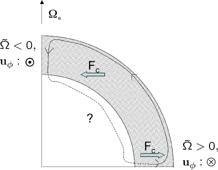
Figure 1: Illustration of gyroscopic pumping in a star with an outer convection zone (shaded area). Slower rotating regions near the poles pump the fluid towards the rotation axis through the action of the Coriolis force (${\bf F}_{\rm c}$) while the rapidly rotating region near the equator pump the fluid away from the rotation axis. A large-scale circulation is thus driven, poleward near the surface. The position of the return flow depends on the radiative zone physics (see GAA09 and §1.2 for detail).

1.2 Mixing in radiative regions induced by gyroscopic pumping

The first quantitative study of gyroscopic pumping in the context of stellar interiors was recently presented by GAA09. They focused on the solar case, i.e. a star with an outer convective region and an inner radiative region, and worked in the Boussinesq approximation (arguing that the solar radiative zone does not span too many pressure and density scaleheights). They showed that the fate of gyroscopically pumped flows – how much overall mixing they induce beyond the convective zone – depends equally on the thermal stratification and on the dynamical properties of the nearby radiative region.

In accordance with the earlier results of Garaud & Brummell (2008), they found that in stratified, rotating stars in quasi-steady dynamical balance, the effect of stratification on large-scale meridional flows is principally controlled by the quantity

$$\sigma=\sqrt{\rm Pr}\frac{N}{\Omega_{\star}}\mbox{ , }$$ (1)

where Pr $=\nu/\kappa$ is the Prandtl number (where $\nu$ is the local viscosity, and $\kappa$ is the local thermal diffusivity), $N$ is the local Brunt-Väisälä – or buoyancy – frequency and $\Omega_{\star}$ is the mean stellar rotation rate. When $\sigma$ is large, the effect of thermal stratification is strongly felt by the gyroscopically pumped meridional flows, which are exponentially damped away from the radiative–convective interface on the lengthscale $R_{\star}/\sigma$. Correspondingly, if $\sigma$ is small the flows can in principle penetrate much more deeply into the radiative interior, and cause significant large-scale mixing.

It is important to note that $\sigma$ depends on $\Omega_{\star}$, so that the effect of stratification (in the sense defined above) is strongly reduced for rapidly rotating stars. Figure 2 shows an estimate of $\sigma$ for various stars in the mass range $1.3M_{\odot}-1.5M_{\odot}$ at age 300Myr. In all cases, $\sigma$ remains well-below unity showing that large-scale mixing of the radiative zone by gyroscopic pumping could be significant for these stars.

Figure 2: Profile of $\sigma(r)$ for three different stellar masses at age 300Myr. The 1.3$M_{\odot}$, 1.4$M_{\odot}$ and 1.5$M_{\odot}$ stars are assumed to be rotating with the velocities $8\times 10^{-5}$rad/s, $1.3\times 10^{-4}$rad/s, and $1.5\times 10^{-4}$rad/s respectively. The stellar models are computed using a standard stellar evolution code developed by Bodenheimer et al. (2007).

Crucially, however, GAA09 showed that even in the very weakly stratified limit ($\sigma\ll 1$), a second condition needs to be satisfied for the pumped flows to penetrate into the nearby radiative region. Indeed, this limit corresponds to the case where the system’s dynamics are dominated by the balance between the perturbation to the pressure gradient and the Coriolis force. This well-known situation is called the “Taylor-Proudman” state, and (in the Boussinesq approximation) implies that all components of the velocity field are strongly constrained to be constant along the rotation axis. GAA09 showed that the Taylor-Proudman constraint can prohibit flow generated within the outer convection zone from entering the underlying radiative zone. Indeed, by mass conservation, any flows entering the radiative zone must somehow return to the convection zone. But such return flow would necessarily require breaking away from the Taylor-Proudman state. Hence, if there exists a region within the radiative zone where the Taylor-Proudman constraint is broken, then this region provides a channel through which the pumped flows can return, as illustrated in Figure 3. If such a region does not exist, the meridional flows instead return within the convection zone causing negligible mixing in the radiative zone.

Since the Taylor-Proudman constraint is broken whenever there exist additional stresses of amplitude comparable with the Coriolis force, various mechanisms can be invoked. Of particular interest are Maxwell stresses in the presence of small- or large-scale magnetic fields (see Gough & McIntyre 1998, for example), and turbulent stresses within another convective region. It is the latter we are mostly interested in studying in this work, namely the case of stars with a convective envelope and a convective core.

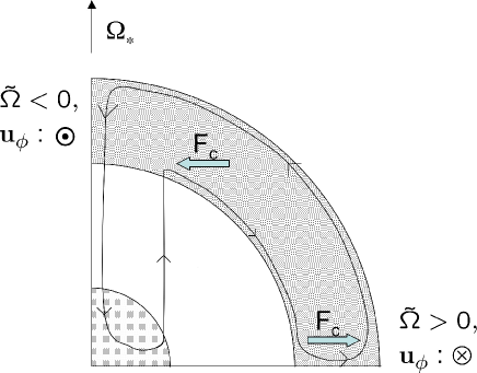
Figure 3: Illustration of the expected flow pattern for rapidly rotating stars with two convective zones. Gyroscopically pumped flows from one convection zone can enter the radiative zone and return within the second convective zone where the Taylor-Proudman constraint does not apply (see main text for detail). Note the role of the tangent cylinder in such a model in delimiting mixed regions from non-mixed regions.

This paper is organized as follows. We first present a fairly exhaustive study of gyroscopic pumping for rapidly rotating stars (in the limit where $\sigma<1$). In §2 we lay out the general formulation of the problem and the assumptions made. Note that the basic model used in this paper is largely inspired from the work of GAA09 but extends it to the case of multiple convective regions and uses a more generally applicable formalism for the fluid dynamics, namely the anelastic approximation. In §3 we first solve the problem analytically in a Cartesian coordinate system, using a much simplified stellar model. This exercise provides insight onto how the meridional flow velocities induced by gyroscopic pumping scale with the forcing mechanism (in this case the differential rotation of the inner and/or outer convection zone), with the stratification within the radiative region, and with the system’s geometry (i.e. the respective widths of the inner and outer convective regions). In §4, we then apply the same model in a two-dimensional spherical geometry, using a more realistic stellar model as the background state. By comparing Cartesian-model results with equivalent spherical-model results, we deduce a very simple rule to go from one to the other. This rule is particularly useful since one-dimensional Cartesian model numerical solutions can be obtained in a tiny fraction of the time necessary to integrate the two-dimensional spherical case, and can also be pushed to true stellar parameter values (which cannot be done in two dimensions).

Next, we present a simple application of this theory to estimate the surface abundances of lithium (Li) and beryllium (Be) in young Main Sequence stars as a function of their age and mass. More precisely, we are interested in young stars in the mass range of $1.3M_{\odot}-1.5M_{\odot}$, which have the well-known property of being significantly depleted in Li and Be in their surface layers as compared with slightly more and slightly less massive stars (Boesgaard & Tripico 1986; see Boesgaard 2005 and Anthony-Twarog et al. 2009 for reviews). These so-called “Li-dip” stars are unique in the sense that they have two significant convection zones (one inner and one outer) which, as described earlier, could promote large-scale mixing between the surface and the interior by gyroscopic pumping. In §5, we show that the Li and Be depletion rates as induced by gyroscopic pumping for Li-dip stars can be very significant. For reasonable model assumptions, the cool (low-mass) side of the dip is readily explained by gyroscopic pumping, while depletion fractions on the hot (high-mass) side are much larger than observed. When the diffusion of chemical species back into the outer convection zone (by overshooting motions for example) is taken into account, good agreement between the model and the data is achieved on both sides of the dip. Finally, we conclude in §6 by summarizing our main results and discussing future prospects.

2 The model

In this section we briefly derive the model equations used throughout this paper. We consider a star of radius $R_{\star}$, rotating with a mean angular velocity $\Omega_{\star}$. In all that follows, we assume that the system is in a quasi-steady state, non-magnetic, and axially symmetric. While these assumptions are probably over-simplistic, they help us narrow down gyroscopic pumping to its essence.

The star considered can have up to two convective regions: a convective core, extending from the center of the star to a first radiative–convective interface located at the radius $r=r_{\rm in}$; and a convective envelope, located between the outer radiative–convective interface at $r=r_{\rm out}$ and the surface. Note that the stellar surface and both interfaces are assumed to be perfectly spherical.

GAA09 studied large-scale meridional flows within the solar interior using the Boussinesq approximation. This approximation treats the thermodynamical quantities as the sum of a weakly varying background plus small perturbations. One may argue in favor of its use in the solar radiative zone, which does not span too many density scaleheights. Here, however, we aim to model stars with very thin outer convective regions, in which case the radiative zone extends nearly all the way to the stellar photosphere. We must therefore switch to using the more general anelastic approximation instead, which allows for a more strongly varying background stratification.

The anelastic approximation implicitly assumes that all velocities are small compared with the local sound speed, and that thermodynamical perturbations are small compared with the equivalent background quantities. We thus define $\bar{p}(r)$, $\bar{\rho}(r)$, $\bar{T}(r)$ and $\bar{s}(r)$ as the spherically symmetric background pressure, density, temperature and entropy profiles, and the equivalent $\tilde{p}$, $\tilde{\rho}$, $\tilde{T}$ and $\tilde{s}$ as two-dimensional perturbations to these quantities. If the equation of state is assumed to be that of a perfect gas (which is an acceptable approximation for the purpose of this work), then the perturbations are related by

$$\frac{\tilde{p}}{\bar{p}}=\frac{\tilde{\rho}}{\bar{\rho}}+\frac{\tilde{T}}{\bar{T}}\mbox{ , }$$ (2)

neglecting for simplicity the dependence on the chemical gradients.

The momentum, thermal energy and mass conservation equations describing the dynamics of the interior flows and thermodynamical perturbations, in the anelastic approximation, are:

$${\bf u}\cdot\nabla{\bf u}+2{\bf\Omega}_{\star}\times{\bf u}=-\frac{\nabla\tilde{p}}{\bar{\rho}}+\frac{\tilde{\rho}}{\bar{\rho}}\bar{\bf g}+\frac{1}{\bar{\rho}}\nabla\cdot\Pi\mbox{ , }$$

$$\bar{\rho}\bar{c}_{p}\bar{T}{\bf u}\cdot\nabla\bar{s}=\nabla\cdot(\bar{k}_{T}\nabla\tilde{T})-\nabla\cdot F_{T}\mbox{ , }$$

$${\mathbf{\nabla}}\cdot(\bar{\rho}{\bf u})=0\mbox{ , }$$ (3)

where ${\bf u}$ is the velocity field expressed in a frame rotating with angular velocity $\Omega_{\star}$, $\bar{\bf g}=(0,0,-\bar{g})$ is gravity, $\Pi$ is the viscous stress tensor, $\bar{c}_{\rm p}$ is the specific heat at constant pressure, $\bar{k}_{T}=\bar{\rho}\bar{c}_{\rm p}\bar{\kappa}$ is the thermal conductivity and finally $F_{T}$ is the turbulent heat flux (in the convective regions). Note that we have neglected any distortion of the star caused by the centrifugal force, as well as perturbations to the gravitational field. These assumptions suppress the well-known global Eddington-Sweet flows (see Spiegel & Zahn 1992).

Following GAA09, we model the inertial term of the momentum equation in the convective regions by the sum of a turbulent viscosity plus a linear drag term driving the system toward a differentially rotating profile: $-({\bf u}-u_{\rm cz}{\bf e}_{\phi})/\tau$, where $u_{\rm cz}{\bf e}_{\phi}$ is the assumed/observed azimuthal velocity profile in the convective zones and where $\tau$ is the local convective turnover timescale (which varies with depth). This drag term is introduced to “mimic” the effect of turbulent convection on driving differential rotation. It is only significant in the convection zones, and drops to zero in the radiative region. The very slow flow velocities expected in the radiative zone justify neglecting the various nonlinear terms in the momentum and heat equation there. We replace the turbulent heat advection term by a turbulent diffusivity, which is assumed to be very large in the convection zones and rapidly tends to zero otherwise.

The resulting model equations, which we use throughout this work unless otherwise specified, are therefore:

$$2{\bf\Omega}_{\star}\times{\bf u}=-\frac{\nabla\tilde{p}}{\bar{\rho}}+\frac{\tilde{\rho}}{\bar{\rho}}\bar{\bf g}+\frac{1}{\bar{\rho}}\nabla\cdot\left(\Pi+\Pi_{\rm turb}\right)-\frac{{\bf u}-u_{\rm cz}{\bf e}_{\phi}}{\tau}\mbox{ , }$$

$$\frac{\bar{\rho}\bar{c}_{p}\bar{T}\bar{N}^{2}}{g}{\bf u}\cdot{\bf e}_{r}=\nabla\cdot((\bar{k}_{T}+k_{\rm turb})\nabla\tilde{T})\mbox{ , }$$

$$\frac{\tilde{p}}{\bar{p}}=\frac{\tilde{\rho}}{\bar{\rho}}+\frac{\tilde{T}}{\bar{T}}\mbox{ , }$$

$${\mathbf{\nabla}}\cdot(\bar{\rho}{\bf u})=0\mbox{ , }$$ (4)

where $\Pi_{\rm turb}$ is similar to the microscopic stress tensor, but using a turbulent viscosity instead. Note that we have rewritten the background heat advection term to emphasize the dependence on the buoyancy frequency $\bar{N}$ (see Spiegel & Zahn 1992, for example).

3 A simplified Cartesian model

Much can be learned about the dynamics of stellar interiors by first studying a simplified problem in Cartesian geometry (the “planar star” approximation, see Garaud & Brummell 2008 and GAA09 for example). Equations in this geometry can usually be solved analytically to gain insight into the physical processes at play. They often reveal important scaling laws governing the solutions, and finally, are rarely more than an “order one” geometrical factor away from more realistic solutions in spherical geometry (in fact we prove this in §4). Our primary goals in this section are therefore not quantitative. Rather, we aim to determine, qualitatively, how deeply the meridional flow velocities generated by gyroscopic pumping penetrate into the radiative zone, and characterize how their amplitude scales with the system parameters.

Since the Cartesian model solutions obtained are knowingly off by a factor of order unity anyway, we further simplify the equations, in this section only, with the following substitutions:

$$\frac{1}{\bar{\rho}}{\mathbf{\nabla}}\cdot(\Pi+\Pi_{\rm turb})\rightarrow(\bar{\nu}+\nu_{\rm turb}){\mathbf{\nabla}}^{2}{\bf u}\mbox{ , }$$

$$\nabla\cdot\left((\bar{k}_{T}+k_{\rm turn})\nabla\tilde{T}\right)\rightarrow(\bar{k}_{T}+k_{\rm turb})\nabla^{2}\tilde{T}\mbox{ . }$$ (5)

It can be shown (through numerical integrations) that neither of these substitutions affect the scalings of the solutions in the case where both convection zones are present. Finally, and following Spiegel & Zahn (1992) we neglect in this section, for analytical simplicity, the pressure perturbations in the linearized equation of state so that:

$$\frac{\tilde{\rho}}{\bar{\rho}}=-\frac{\tilde{T}}{\bar{T}}\mbox{ . }$$ (6)

3.1 Model setup and non-dimensional equations

As in GAA09, we consider a Cartesian coordinate system $(x,y,z)$ with $z$ aligned with both gravity and with the rotation axis. The $x$-direction represents the azimuthal direction, while the $y$-direction is equivalent to minus the co-latitude. Distances are normalized to the stellar radius $R_{\star}$, so that the stellar interior is in the interval $z\in[0,1]$, the inner convection zone spans the interval $[0,z_{\rm in}]$ and the outer convection zone spans $[z_{\rm out},1]$. Figure 4 illustrates the geometry of the Cartesian system. We assume that the star is axially symmetric, i.e. independent of $x$, and periodic in $y$ on the interval $[0,\pi]$ (representing the two “poles”) with equatorial symmetry (i.e. symmetric about $y=\pi/2$).

Figure 4: Cartesian model geometry and intended correspondence with the spherical case. The shaded area marks the convective regions, where forcing is applied. The $y=0$ and $y=\pi/2$ lines mark the “poles” and the “equator”. The system is assumed to be periodic with period $\pi$ in the $y-$direction.

The background stellar model is chosen to be very simple, so that analytical solutions of the problem can easily be found. We take

• $\bar{\rho}(z)=\rho_{c}e^{-z/D_{\rho}}$ and $\bar{T}(z)=T_{c}e^{-z/D_{T}}$,

• $\bar{\nu}$, $\bar{\kappa}$ and $\bar{g}$ are constant.

Note that fits to actual stellar models show that the non-dimensional density and temperature scaleheights typically satisfy the inequalities $D_{\rho}\ll D_{T}<1$.

The global velocity field in the rotating frame is ${\bf u}=(u,v,w)$ and flow velocities are normalized to $R_{\star}\Omega_{\star}$. In this framework, the unit timescale is $\Omega_{\star}^{-1}$. Density and temperature perturbations are normalized by $\rho_{c}$ and $\epsilon T_{c}$ respectively, where $\epsilon=R_{\star}\Omega_{\star}^{2}/\bar{g}$ is the ratio of the centrifugal force to gravity. Pressure perturbations are normalized to $\rho_{c}R^{2}_{\star}\Omega_{\star}^{2}$. The set of equations (2) then simplifies to the non-dimensional system:

$$2{\bf e}_{z}\times{\bf u}=-\nabla\tilde{p}\,e^{z/D_{\rho}}+\tilde{T}e^{z/D_{T}}{\bf e}_{z}+(E_{\nu}+E_{\nu,{\rm turb}}){\mathbf{\nabla}}^{2}{\bf u}-\frac{{\bf u}-{\bf u}_{\rm cz}}{\tau}\mbox{ , }$$

$$\frac{\bar{N}^{2}}{\Omega_{\star}^{2}}e^{-z/D_{T}}w=(E_{\kappa}+E_{\kappa,{\rm turb}})\nabla^{2}\tilde{T}\mbox{ , }$$

$${\mathbf{\nabla}}\cdot(e^{-z/D_{\rho}}{\bf u})=0\mbox{ , }$$ (7)

where we have introduced a series of standard parameters, namely the Ekman number

$$E_{\nu}=\frac{\bar{\nu}}{R_{\star}^{2}\Omega_{\star}}\mbox{ , }$$ (8)

and the equivalently defined $E_{\nu,{\rm turb}}$, as well as

$$E_{\kappa}=\frac{\bar{\kappa}}{R_{\star}^{2}\Omega_{\star}}\mbox{ , }$$ (9)

which is actually an inverse Peclet number, and the equivalently defined $E_{\kappa,{\rm turb}}$. Note that the microscopic diffusivities normally vary with depth within a star, but are assumed here to be constant for simplicity. Deep within the interiors of Hyades-age stars in the Li-dip mass range,

$$E_{\nu}\sim 10^{-17}-10^{-15}\mbox{ , }E_{\kappa}\sim 10^{-12}-10^{-7}\mbox{ . }$$ (10)

In order to fully specify the model, the functions $\bar{N}(z)$, $\tau(z)$, $u_{\rm cz}(y,z)$ and the turbulent diffusivity profiles must be selected. The buoyancy frequency is taken to be

$$\bar{N}(z)=\frac{N_{\rm rz}}{2}\left[\tanh\left(\frac{z_{\rm out}-z}{\Delta_{\rm out}}\right)+\tanh\left(\frac{z-z_{\rm in}}{\Delta_{\rm in}}\right)\right]\mbox{ , }$$ (11)

so that $\bar{N}(z)\rightarrow 0$ in both convection zones, and $\bar{N}(z)\simeq N_{\rm rz}$ in the radiative zone. The lengthscales $\Delta_{\rm in}$ and $\Delta_{\rm out}$ may be thought of as the respective thicknesses of the “overshoot” regions located near each of the two convection zones (and in this section are taken to be equal to one another, for simplicity). For $\tau(z)$, we take

$$\tau(z)^{-1}=\frac{\Lambda_{\rm in}}{2}\left[1+\tanh\left(\frac{z_{\rm in}-z}{\Delta_{\rm in}}\right)\right]+\frac{\Lambda_{\rm out}}{2}\left[1+\tanh\left(\frac{z-z_{\rm out}}{\Delta_{\rm out}}\right)\right]\mbox{ , }$$ (12)

where $\Lambda_{\rm in}$ and $\Lambda_{\rm out}$ are assumed to be constant and equal to the inverse of the (non-dimensional) convective turnover time in the relevant convection zone.

Both convective zones may be differentially rotating. For mathematical simplicity again, we assume in this Cartesian model that their latitudinal dependence is similar. We therefore select the following functional form for $u_{\rm cz}(y,z)$:

$$u_{\rm cz}(y,z)=\hat{u}_{\rm cz}(z)e^{iky}\mbox{ , }$$ (13)

where $k=2$ to guarantee equatorial symmetry. The radial profile $\hat{u}_{\rm cz}(z)$ is then chosen to be

$$\hat{u}_{\rm cz}(z)=\frac{\hat{u}_{\rm cz}^{\rm out}(z)}{2}\left[1+\tanh\left(\frac{z-z_{\rm out}}{\Delta_{\rm out}}\right)\right]+\frac{\hat{u}_{\rm cz}^{\rm in}(z)}{2}\left[1+\tanh\left(\frac{z_{\rm in}-z}{\Delta_{\rm in}}\right)\right]\mbox{ . }$$ (14)

The functions $\hat{u}_{\rm cz}^{\rm out}(z)$ and $\hat{u}_{\rm cz}^{\rm in}(z)$ can a priori depend on depth (see GAA09 for example). By analogy, the non-dimensional turbulent diffusivity profiles are constructed as

$$E_{\nu,{\rm turb}}(z)=\frac{E^{\rm out}_{\nu,{\rm turb}}(z)}{2}\left[1+\tanh\left(\frac{z-z_{\rm out}}{\Delta_{\rm out}}\right)\right]+\frac{E^{\rm in}_{\nu,{\rm turb}}(z)}{2}\left[1+\tanh\left(\frac{z_{\rm in}-z}{\Delta_{\rm in}}\right)\right]\mbox{ , }$$ (15)

and similarly for $E_{\kappa,{\rm turb}}(z)$.

Projecting the model equations into Cartesian coordinates, using invariance in the $x-$direction and seeking periodic solutions in the form of $q(y,z)=\hat{q}(z)e^{iky}$ for each of the dependent variables yields:

$$-2\hat{v}=(E_{\nu}+E_{\nu,{\rm turb}})\left(\hat{u}_{zz}-k^{2}\hat{u}\right)-\frac{\hat{u}-\hat{u}_{\rm cz}}{\tau}\mbox{ , }$$

$$2\hat{u}=-ik\hat{p}e^{z/D_{\rho}}+(E_{\nu}+E_{\nu,{\rm turb}})\left(\hat{v}_{zz}-k^{2}\hat{v}\right)-\frac{\hat{v}}{\tau}\mbox{ , }$$

$$0=-\hat{p}_{z}e^{z/D_{\rho}}+\hat{T}e^{z/D_{T}}+(E_{\nu}+E_{\nu,{\rm turb}})\left(\hat{w}_{zz}-k^{2}\hat{w}\right)-\frac{\hat{w}}{\tau}\mbox{ , }$$

$$\frac{\bar{N}^{2}}{\Omega_{\star}^{2}}e^{-z/D_{T}}\hat{w}=(E_{\kappa}+E_{\kappa,{\rm turb}})\left(\hat{T}_{zz}-k^{2}\hat{T}\right)$$

$$ik\hat{v}e^{-z/D_{\rho}}+(e^{-z/D_{\rho}}\hat{w})_{z}=0\mbox{ . }$$ (16)

where the subscript $z$ denotes a derivative with respect to $z$.

Finally, we need to specify an adequate set of boundary conditions for the system. The two boundaries at $z=0$ and $z=1$ are assumed to be impermeable ($\hat{w}=0$), stress-free ($\hat{u}_{z}=\hat{v}_{z}=0$), and the temperature perturbations are assumed to be zero. Note that as long as the system boundaries are located in a convective region, the actual choice of boundary conditions has little influence on the result.

3.2 Solution and interpretation of the model

The set of equations (16) and associated boundary conditions (see above) can be solved analytically when the overshoot regions are very thin compared with the depths of the respective convective zones. The complete derivation of the solution is fairly straightforward although algebraically cumbersome. It is detailed in Appendix A: exact solutions are derived in each of the three regions $[0,z_{\rm in}]$, $[z_{\rm in},z_{\rm out}]$ and $[z_{\rm out},1]$, and matched to one another across the radiative–convective interfaces at $z_{\rm in}$ and $z_{\rm out}$ respectively. In what follows, we discuss the most important outcome of this analysis, namely the prediction of the gyroscopically pumped mass flux mixing the radiative zone.

3.2.1 General behavior of the model solutions.

As found by GAA09, in the limit where $\sigma<1$ the meridional flows generated in the convective regions can penetrate deeply into the nearby radiative zone. A very simple way of seeing this is to note that in this limit, the $x-$component of the momentum equation in (16) reduces to $\hat{v}=O(E_{\nu})$ in the radiative zone which then implies, by mass conservation, that

$$(e^{-z/D_{\rho}}\hat{w})_{z}=O(E_{\nu})\mbox{ . }$$ (17)

Hence the non-dimensional vertical mass flux mixing the radiative zone, $\bar{\rho}\hat{w}$, is constant along the rotation axis:

$$\bar{\rho}\hat{w}=W_{\rm rz}\mbox{ , }$$ (18)

and spans the entire region, extending from one convection zone to the other as drawn in Figure 3 for example.

The details of the calculation of the pumped mass flux $W_{\rm rz}$, even for this simplified stellar model, are fairly complicated and are presented in Appendix A. In the limit where the depths of both convection zones $d_{\rm in}=z_{\rm in}$ and $d_{\rm out}=1-z_{\rm out}$ are small compared with the stellar radius (which is true for most stars in the Li dip), we show that

$$W_{\rm rz}=\frac{2}{k}\frac{P}{\frac{N_{\rm rz}^{2}}{\Omega_{\star}^{2}}\frac{G}{E_{\kappa}}-\frac{1}{k^{2}}\left(\frac{4+\Lambda_{\rm in}^{2}}{\Lambda_{\rm in}d_{\rm in}}+\frac{4+\Lambda_{\rm out}^{2}}{\Lambda_{\rm out}d_{\rm out}}\right)}\mbox{ , }$$ (19)

where $P$ is the “pumping term”

$$P = \bar{\rho}(z_{\rm out})u_{\rm cz}^{\rm out}(z_{\rm out})-\bar{\rho}(z_{\rm in})u_{\rm cz}^{\rm in}(z_{\rm in})+d_{\rm out}\left.\frac{{\rm d}(\bar{\rho}u^{\rm out}_{\rm cz})}{{\rm d}z}\right|_{z=z_{\rm out}}+d_{\rm in}\left.\frac{{\rm d}(\bar{\rho}u^{\rm in}_{\rm cz})}{{\rm d}z}\right|_{z=z_{\rm in}}\mbox{ , }$$ (20)

and where $G$ is the following fairly obscure factor:

$$G=L^{2}(z_{\rm out}-z_{\rm in})$$ (21)

$$- kL^{4}\left[1-\frac{2L}{d_{\rm out}}+\frac{2L}{d_{\rm out}}e^{-d_{\rm out}/L}\right]\left[\frac{e^{k}}{\sinh(k)}\left(1+\frac{d_{\rm out}}{L}\right)-\frac{e^{-(z_{\rm out}-z_{\rm in})/L}}{\sinh(k)}\left(1-\frac{d_{\rm in}}{L}\right)-\frac{1}{kL}\right]$$

$$+ kL^{4}\left[1+\frac{2L}{d_{\rm in}}-\frac{2L}{z_{\rm in}}e^{z_{\rm in}/L}\right]\left[\frac{e^{(z_{\rm out}-z_{\rm in})/L}}{\sinh(k)}\left(1+\frac{d_{\rm out}}{L}\right)-\frac{e^{-k}}{\sinh(k)}\left(1-\frac{d_{\rm in}}{L}\right)-\frac{1}{kL}\right]\mbox{ ,}$$

where

$$L^{-1}=D_{\rho}^{-1}-D_{T}^{-1}\mbox{ .}$$ (22)

Note that $G$ is found to be negative for all reasonable parameter values, so that the denominator of (19) never vanishes. Our analytical solution is easily verified by comparison with numerical solutions of the full set of equations (16), as shown in §3.2.3. However, let us first attempt to understand the meaning of (19) on physical grounds.

3.2.2 Interpretation of the dependence of the pumped mass flux on physical parameters

This expression for $W_{\rm rz}$ calculated in §3.2.1 can be interpreted more easily in two different asymptotic limits.

The unstratified limit.

When $N_{\rm rz}\rightarrow 0$ (the unstratified limit), $W_{\rm rz}$ takes the simpler form:

$$|W_{\rm rz}|=\frac{2}{k}\frac{P}{\frac{4+\Lambda_{\rm in}^{2}}{\Lambda_{\rm in}d_{\rm in}}+\frac{4+\Lambda_{\rm out}^{2}}{\Lambda_{\rm out}d_{\rm out}}}\mbox{ . }$$ (23)

We see that $W_{\rm rz}$ is roughly of the order of the pumping term, times a factor which depends only on the respective properties (depth, convective turnover time) of the convective zones. Our main conclusion is that the mass flux into the radiative zone appears to go to zero if one of the convection zones vanishes, either by becoming vanishingly thin ($d_{\rm in}$ or $d_{\rm out}\rightarrow 0$), or if the associated convective stresses become negligible ($\Lambda_{\rm in}$ or $\Lambda_{\rm out}\rightarrow 0$).

This important result can in fact be easily understood in the light of the work of GAA09 described in §1.2. Indeed, in the unstratified case, radiative zone flows must satisfy the Taylor-Proudman constraint. Any flows generated by gyroscopic pumping in one convection zone can only enter the radiative zone if there is a return path at the other end. If the second convective zone vanishes, this return path is no longer available. The flows instead return within the existing convection zone, and do not mix the radiative region significantly. The stratified case with $\sigma<1$ is very similar.

Based on these very simple considerations, we can therefore expect that the overall mixing rate in the star resulting from gyroscopic pumping must reach a maximum for a given stellar mass between $1M_{\odot}$ (no or negligible convective core) and $1.8M_{\odot}$ (no or negligible convective envelope). This simple idea motivated our study of the Li dip (see §5), although, as we shall show, the real problem is much more subtle.

The stratified case.

The unstratified limit discussed above is of course artificial. In real stars $N_{\rm rz}\neq 0$ and one must instead compare the two terms in the denominator of (19) to one another. In the limit where the first term is much larger than the second then

$$|W_{\rm rz}|\simeq\frac{2P}{k}\frac{E_{\kappa}}{G}\frac{\Omega_{\star}^{2}}{N_{\rm rz}^{2}}\mbox{ . }$$ (24)

The flow velocities pumped into the radiative zone are now found to follow a local Eddington-Sweet scaling law, which is not surprising since we are looking at quasi-steady flows in a stratified fluid driven by rotational forcing. Such solutions were already found by Spiegel & Zahn (1992) for example in the case of the Sun. Naturally, local Eddington-Sweet flows are much slower than the flows pumped through each individual convective zone, although they could still provide significant sources of mixing in fairly rapidly rotating stars.

The effect discussed in the unstratified case, namely the complete suppression of $W_{\rm rz}$ in the limit where one of the convection zone disappears, still occurs but only when

$$\frac{\sigma^{2}G}{E_{\nu}}=\frac{N_{\rm rz}^{2}}{\Omega_{\star}^{2}}\frac{G}{E_{\kappa}}\ll\frac{1}{k^{2}}\left(\frac{4+\Lambda_{\rm in}^{2}}{\Lambda_{\rm in}d_{\rm in}}+\frac{4+\Lambda_{\rm out}^{2}}{\Lambda_{\rm out}d_{\rm out}}\right)\mbox{ .}$$ (25)

Since $N_{\rm rz}^{2}/E_{\kappa}\Omega_{\star}^{2}$ is typically very large because $E_{\kappa}$ is very small, this limit is only relevant for extremely thin or weak convective regions.

Based on these considerations, we can now re-interpret (19) in the following way: $W_{\rm rz}$ has two strict upper limits: a first upper limit, which arises from mechanical constraints (by the driving force and the Taylor-Proudman constraint), and a second upper limit which arises from the thermal stratification of the system (which can strongly suppress radial flows). The actual value of $W_{\rm rz}$ mixing the radiative zone is the smaller of the two, thus defining two different regimes, the “unstratified” regime (where $W_{\rm rz}$ is mechanically constrained) and the “weakly stratified” regime (where $W_{\rm rz}$ is thermally constrained).

3.2.3 Comparison with full solutions of the governing equations

In this section we verify the analytical solution for $W_{\rm rz}$ expressed in (19) by comparison with numerical solutions of the same equations. Numerical solutions are obtained by integrating the two-point boundary value problem (16) with associated boundary conditions, background state and forcing as specified in §3.2.1.

A direct comparison of the analytical and numerical solutions for $W_{\rm rz}$ is shown in Figure 5, for a wide range of simulations. For all the calculations presented, the microscopic diffusion parameters $E_{\nu}=10^{-7}$ and the Prandtl number Pr = $E_{\nu}/E_{\kappa}=10^{-2}$ are fixed. The turbulent diffusivities are set to 0 for simplicity. For the forcing by the differential rotation, as expressed in (14), we take $\hat{u}_{\rm cz}^{\rm out}(z)=\hat{u}_{\rm cz}^{\rm in}(z)=u_{0}$ and $\Lambda_{\rm in}=\Lambda_{\rm out}=10$. Note that the problem is linear so the value of $u_{0}$ is irrelevant. The overshoot depths are taken to be $\Delta_{\rm in}=\Delta_{\rm out}=10^{-4}$. The background density and temperature scaleheights are selected to be $D_{\rho}=0.075$ and $D_{T}=0.275$, so that $L=0.1$. Note that these scaleheights are a good approximation to the true density and temperature scaleheights in the radiative zones of stars in the $1.3M_{\sun}-1.5M_{\sun}$ range. The non-dimensional buoyancy frequency of the radiative zone $N_{\rm rz}/\Omega_{\star}$ is varied for each set of simulations, leading to $\sigma$ ranging from $10^{-4}$ to 10. Finally, each symbol corresponds to a particular geometry of the system, with different possible pairs of values $(z_{\rm in},z_{\rm out})$ as shown.

For each simulation the quantity $\bar{\rho}\hat{w}$ is measured from the numerical solution at $z=0.5$. Note that for $\sigma<1$, $\bar{\rho}\hat{w}$ is found to be constant across much of the radiative zone (as expected), so exactly where $\bar{\rho}\hat{w}$ is measured does not matter much. For $\sigma\geq 1$, $\bar{\rho}\hat{w}$ is no longer constant, so the specific height $z=0.5$ is selected for consistency across simulations.

Figure 5: Comparison between the numerical and analytical results for $W_{\rm rz}=\bar{\rho}\hat{w}$. For each selected value of $\sigma$ ranging from $10^{-4}$ to 10, two sets of simulations are shown with different convection zone depths: the case of thinnest convection zones ($z_{\rm in}=0.05$, $z_{\rm out}=0.95$) is shown as diamond symbols, while ($z_{\rm in}=0.15$, $z_{\rm out}=0.85$) is shown as squares. The corresponding analytical solutions are shown as dotted and solid lines respectively. For $\sigma<1$ the numerical and analytical results fit very well for all cases, showing that the approximate formula for $W_{\rm rz}$ (see equation (19)) applies. For $\sigma>1$ the formula doesn’t do so well, as expected.

We find that the analytical solution (19), shown in the dotted and solid lines, fits the numerical results very well as long as $\sigma<1$. The mismatch for $\sigma>1$ was expected because we can no longer assume that $\bar{\rho}\hat{w}$ is constant across the radiative zone (see GAA09 for example), while this is key to the derivation of (19). Figure 5 also shows the two regimes discussed in §3.2.3. In the “unstratified limit”, for $\sigma\rightarrow 0$, we observe a plateau in $W_{\rm rz}$ which sets the largest achievable value for flows in the interior. As the degree of stratification increases, the flows driven into the radiative zone are slowed down by the local thermal stratification, a phenomenon which becomes more pronounced as $N_{\rm rz}$ increases (equivalently, as $\sigma$ increases). The flow velocities in this “weakly stratified” regime scale as $\sigma^{-2}$, which is equivalent to the aforementioned local Eddington-Sweet scaling since $E_{\nu}$ and Pr are constant. Note that in this regime, the flow pattern still spans the entire region with constant $\bar{\rho}\hat{w}$.

3.3 Summary

To summarize this section, we have used a simple toy model to study how gyroscopic pumping by convective zone stresses induces large-scale meridional fluid motions. We found that the pumping indeed drives significant large-scale flows within the convection zone(s) (see GAA09). Furthermore, in some circumstances, a fraction of the pumped mass flux may enter the adjacent radiative zone, and induce a circulation of material with the following properties:

• Convection zone flows penetrating into the nearby radiative zone are exponentially damped on a lengthscale $R_{\star}/\sigma$ where $\sigma$ is given by equation (1). If $\sigma<1$ (which is the case for most rapid rotators) the flows can potentially mix the entire star (Garaud & Brummell 2008, GAA09).

• In the limit $\sigma<1$ the pumped mass flux within the radiative zone $\bar{\rho}\hat{w}$ is mechanically constrained to be constant along the rotation axis.

• The fraction of the gyroscopically pumped mass flux which does enter the radiative zone (by contrast with the mass flux which returns immediately within the driving convection zone) is capped by the lowest of two constraints: a mechanical constraint, which crucially depends on the presence of another source of stresses somewhere else within the system to enable flows to return to their point of origin (see previous sections for detail, as well as GAA09), and a thermal constraint, which limits the flow velocities to local Eddington-Sweet velocities. Note that this second constraint was not discussed by GAA09, but turns out to be the most relevant one for most stars.

The efficiency of gyroscopic pumping on mixing stellar interiors thus depends on many factors, including the background stellar structure, the thermal diffusivity, the stellar rotation rate and the nature of the convective zone stresses. However, thanks to the analytical formula (19), we now have a reasonably clear picture of precisely how all of these factors influence the amplitude of the gyroscopically pumped mass flux within a star.

4 From Cartesian to Spherical models

The next step of this investigation is to move to more realistic numerical simulations of the problem in a spherical geometry. We have two goals in this endeavour. The first is to understand the effect of the spherical geometry on the solutions. In particular, we are interested in the dichotomy between the regions located respectively within and outside of the cylinder tangent to the convective core and aligned with the rotation axis (see Figure 3). The second goal is much more quantitative, and is to extract (if possible) simple laws relating the calculated mass flux $W_{\rm rz}$ in the Cartesian case to its equivalent in the spherical case. Since Cartesian solutions are much easier to calculate than spherical geometry solutions, a simple rule to go from one set of solutions to the other could prove particularly useful later.

4.1 Model description

The spherical model used is very similar to the model presented in GAA09. The salient points are repeated here for completeness.

We consider a spherical coordinate system $(r,\theta,\phi)$ where $\theta=0$ denotes the rotation axis and $\theta=\pi/2$ marks the equator. The governing equations are the original ones (2) derived in §2. Since we are principally interested in studying the effects of the spherical geometry on the model predictions for the large-scale flow amplitudes, we consider “hypothetical stars” instead of real stellar models. This largely facilitates the comparison between the various simulation outputs, and enables us to focus on how the model depends on specific control parameters.

In all cases, the “star” used is a solar-type star ($R_{\star}=R_{\sun}$, $M_{\star}=M_{\sun}$), and the background thermodynamical quantities such as density, pressure, and temperature ($\bar{\rho}(r)$, $\bar{p}(r)$ and $\bar{T}(r)$ respectively) are extracted from Model S of Christensen-Dalsgaard et al. (1996). However, to model cases with various size convection zones, we create artificial profiles of the buoyancy frequency by using the expression

$$\bar{N}^{2}(r)=N^{2}_{\rm rz}\sin\left(\frac{\pi(r-r_{\rm in})}{r_{\rm out}-r_{\rm in}}\right)\mbox{ if }r\in[r_{\rm in},r_{\rm out}]\mbox{ , }$$

$$\bar{N}^{2}(r)=-10^{-11}\mbox{ otherwise, }$$ (26)

where $r_{\rm in}$ is the radius of the lower radiative–convective interface, and $r_{\rm out}$ is the radius of the upper radiative–convective interface. The maximum value of $\bar{N}(r)$ within the radiative zone, $N_{\rm rz}$, is one of our input parameters, while that of the convection zones is merely chosen to be arbitrarily low and has little effect on the outcome of the simulation. In what follows, we define the global parameter $\sigma_{\star}$ as

$$\sigma_{\star}=\sqrt{{\rm Pr}}\frac{N_{\rm rz}}{\Omega_{\star}}\mbox{ . }$$ (27)

Note that the Prandtl number is assumed to be constant (see below).

In all simulations, the star is assumed to be rotating at the mean angular velocity $\Omega_{\star}=3\times 10^{-4}$rad/s. In all cases, the applied forcing by differential rotation is

$${\bf u}_{\rm cz}(r,\theta)=\frac{r\sin\theta\Omega_{\rm cz}(\theta)}{2}\left[2+\tanh\left(\frac{r-r_{\rm out}}{\Delta_{\rm out}}\right)+\tanh\left(\frac{r_{\rm in}-r}{\Delta_{\rm in}}\right)\right]\mbox{ }{\bf e}_{\phi}\mbox{ , }$$ (28)

where

$$\Omega_{\rm cz}(\theta)=\Omega_{\rm eq}\left(1-a_{2}\cos^{2}\theta\right)\mbox{ , }$$ (29)

with

$$a_{2}=0.01\mbox{ and }\Omega_{\rm eq}=\Omega_{\star}\left(1-\frac{3a_{2}}{15}\right)^{-1}\mbox{ , }$$ (30)

to ensure that the total applied angular momentum to the system is zero. Note that for simplicity, the same differential rotation is chosen in both convection zones, and is measured by the parameter $a_{2}$. This value is chosen to be fairly small, since the observed differential rotation of rapidly rotating stars is typically quite small. In practice, since we are studying a linear problem, the solutions scale linearly with $a_{2}$. Finally, the expression for the non-dimensional quantity $\tau(r)$ is the same as that given in (12) with $\Lambda_{\rm in}=\Lambda_{\rm out}=10$ in both inner and outer convection zones.

The total diffusivities (i.e. the sum of the microscopic and turbulent components) are assumed to have the following profiles:

$$\bar{\kappa}(r)+\kappa_{\rm turb}(r)=\kappa_{c}e^{r/D_{\kappa}}+\frac{\kappa_{\rm turb}}{2}\left[2+\tanh\left(\frac{r-r_{\rm out}}{\Delta_{\rm out}}\right)+\tanh\left(\frac{r_{\rm in}-r}{\Delta_{\rm in}}\right)\right]\mbox{ ,}$$

$$\bar{\nu}(r)+\nu_{\rm turb}(r)={\rm Pr}\,(\bar{\kappa}(r)+\kappa_{\rm turb}(r))\mbox{ .}$$ (31)

The selected exponential profile for the microscopic part of $\bar{\kappa}(r)$ is not too dissimilar from that of a real star in the 1.3-1.5$M_{\odot}$ range provided $D_{\kappa}/R_{\star}=0.14$. We define the inverse Peclet number $E_{\kappa c}=\kappa_{c}/R_{\star}^{2}\Omega_{\star}$. The value of $E_{\kappa c}$ will be varied in the various simulations, and decreased as much as possible to reach the asymptotic stellar regime. We take the Prandtl number to be constant and equal to Pr$=10^{-2}$. The selected value of Pr is chosen to be smaller than one to respect stellar conditions, but larger than the actual stellar values (which are of order of $10^{-6}$ typically) to ease the numerical computations. The “convective” value $\kappa_{\rm turb}$ is fixed so that the non-dimensional $E_{\kappa,{\rm turb}}$ is equal to $10^{-1}$. The overshoot layer depths $\Delta_{\rm in}$ and $\Delta_{\rm out}$ are taken to be 0.01. While these choices are fairly arbitrary, they are reasonable given our qualitative goals.

The computational domain is a spherical shell with the outer boundary located at $0.95R_{\star}$ and the inner boundary at $0.01R_{\star}$. The outer boundary is chosen to be well-below the stellar surface to avoid numerical complications related to the very rapidly changing background in the region $r>0.95R_{\star}$. The inner boundary is chosen to be well-within the inner convection zone, but excludes the origin to avoid coordinate singularities. The upper and lower boundaries are assumed to be impermeable and stress-free, with $\tilde{T}=0$.

The numerical method of solution is based on the expansion of the governing equations onto the spherical coordinate system, followed by their projection onto Chebishev polynomials $T_{n}(\cos\theta)$, and finally, solution of the resulting ODE system in $r$ using a Newton-Raphson-Kantorovich algorithm. The typical solutions shown have 3000 meshpoints and 70 Fourier modes. For more detail on the numerical algorithm, see Garaud (2001) and Garaud & Garaud (2008).

4.2 Typical solution

Solutions have been computed for a wide range of values of the parameters $d_{\rm in}=r_{\rm in}$ and $d_{\rm out}=R_{\star}-r_{\rm out}$ (the respective depths of the inner and outer convection zones), $E_{\kappa c}$ and $\sigma_{\star}$. For low enough diffusivities the overall structure of the radiative zone flows converges to a pattern which only depends on $d_{\rm in}$, $d_{\rm out}$ and $\sigma_{\star}$ (and with an amplitude which scales as the calculated $W_{\rm rz}$). Figure 6 shows a representative example of the kind of 2D flow structure found within the star, for $E_{\kappa c}=10^{-7}$ and $\sigma_{\star}=0.1$. An artificial case with fairly thick convective zones ($r_{\rm in}=0.2R_{\star}$ and $r_{\rm out}=0.8R_{\star}$) was chosen to make it easier to visualise the results.

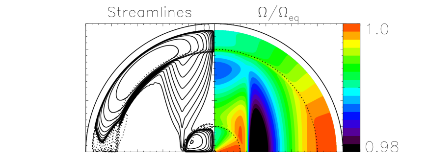
Figure 6: Numerical solution for $r_{\rm out}=0.8R_{\star}$, $r_{\rm in}=0.2R_{\star}$, $E_{\kappa c}=10^{-7}$ and $\sigma_{\star}=0.1$. The two quadrants represent the stellar interior, with the radiative–convective interfaces denoted as dotted circles. The left-side panel shows selected streamlines of the flow, as logarithmically-spaced contours of the stream-function. Solid lines represent clockwise flow, while dotted lines represent counter-clockwise flow. The right-side panel shows the normalized differential rotation profile.

Discussion of the meridional flow structure.

Representative streamlines are shown in the left-side panel of Figure 6 and reveal the structure of the meridional flows driven by gyroscopic pumping. In the outer convection zone, we observe a dominant cell in mid and high latitudes, poleward near the surface and equatorward near $r_{\rm out}$. In addition, a small counter-cell of fairly surprising shape is observed in the equatorial region. The inner convection zone also has a dominant cell of the same vorticity (with poleward flows in the outer layers, and a deep equatorward return flow), and a small counter-cell located just above it along the polar axis. The structure of the two dominant cells in the respective convective zones are easily understood from angular momentum balance. The smaller counter-cell above the inner convection zone is required to match the flows downwelling from the outer convection zone to the inner core flows.

The bulk of the mass flux generated in a given convection zone returns within, or close to the edge of that same convection zone. However, weak flows from the polar region of the outer convective zone, and from the equatorial region of the inner convection zone escape and mix the cylinder tangent to the convective core. Note how, by contrast, the region outside of the tangent cylinder is mostly quiescent.

The variation of the vertical flow amplitude with latitude for the simulation of Figure 6 can be seen more clearly in Figure 7: it illustrates the downward pumping of the flows in the polar regions, while mixing in the equatorial region is mostly negligible. The variation of the amplitude of the flows with depth is well-explained by the variation in the background density: flows pumped downward along the polar axis roughly satisfy $u_{r}=W_{\rm rz}/\bar{\rho}$ (where $u_{r}$ is the radial velocity) where $W_{\rm rz}$ is constant. This constraint is more easily seen in Figure 8 which shows the profile of $\bar{\rho}u_{r}$ at $88^{\circ}$ latitude for the simulation shown in Figure 6. Within the radiative zone we see that $\bar{\rho}u_{r}$ is roughly constant as expected. Figure 8 also illustrates how only a small fraction of the pumped mass flux enters the radiative zone, while most of it remains within the generating convection zone.

Figure 7: Variation of $u_{r}$ with latitude for four different non-dimensional radii $r/R_{\star}$ for the simulation shown in Figure 6. The latitudinal position of the tangent cylinder at each radius is marked by a small diamond. This figure illustrates the polar downwelling, the return flow just outside the tangent cylinder and the mostly negligible mixing at low latitudes. Note that the calculated value of $u_{r}$ should not be taken at face value: it needs to be rescaled appropriately in order to estimate mixing velocities in real stars (see §3.2.1). See §5 for more quantitative estimates in Li-dip stars.

Figure 8: Variation of $\bar{\rho}|u_{r}|$ with depth near the polar axis (at a latitude of $88^{\circ}$) in the simulation of Figure 6. A logarithmic scale is used to visualize simultaneously the convection zone flows and the radiative zone flows. The solid line denotes upwelling flows, while the dashed line denotes downwelling flows. Note the radiative region $r/R_{\star}\in[0.2,0.8]$ where $\bar{\rho}u_{r}$ is constant as expected from the analytical solution.

Discussion of the azimuthal flow structure.

As seen in Figure 6, both convection zones exhibit a rotation profile close to the imposed profile (i.e. with $\Omega/\Omega_{\rm eq}$ ranging from 1-$a_{2}$ to 1 between the pole and the equator, and with $\Omega$ nearly constant with radius), as expected. Meanwhile, the radiative zone exhibits a similar level of differential rotation, with a striking shear layer near the tangent cylinder. This shear is presumably caused by the deposition of negative angular momentum by the meridional flows as they carry fluid away from the rotation axis and begin to rise up in the radiative interior again. Other numerical simulations (not shown here) show that this feature is stronger when flows are stronger, i.e. when the system is more weakly thermally stratified or more rapidly rotating ($\sigma_{\star}$ smaller). An interesting consequence of this shear layer, however, is the possibility that it may become unstable to Rayleigh instabilities in the vicinity of the tangent cylinder, where for extreme cases the specific angular momentum may locally begin to decrease with distance from the polar axis.

4.3 Comparison between Cartesian model predictions and spherical model solutions

The results presented in the previous section show that, for stars with $\sigma_{\star}<1$, the downward pumped mass flux into the radiative zone $W_{\rm rz}$ is indeed constant with depth along the rotation axis, as found in the Cartesian model analysis of §3. We can now compare more quantitatively the results of these spherical simulations with equivalent Cartesian solutions for $W_{\rm rz}$, first in order to verify the scalings derived in (19) and then to see if there exists a simple relationship between the Cartesian model velocities and the spherical model velocities.

We first run a series of two-dimensional spherical simulations, based on the model presented in §4.1, with the following parameters varied:

• We consider three different geometries: $(r_{\rm in}/R_{\star}=0.05,\,r_{\rm out}/R_{\star}=0.9)$ $(r_{\rm in}/R_{\star}=0.1,\,r_{\rm out}/R_{\star}=0.8)$, and $(r_{\rm in}/R_{\star}=0.2,\,r_{\rm out}/R_{\star}=0.8)$. The purpose is to explore the effect of varying the convection zone sizes on the predicted velocities.

• For the case with $r_{\rm in}/R_{\star}=0.1,r_{\rm out}/R_{\star}=0.8$ we consider two different values of $\sigma_{\star}$ (by changing $N_{\rm rz}$): $\sigma_{\star}=0.1$ and $\sigma_{\star}=0.03$. For the other two geometries $\sigma_{\star}$ is fixed to be $0.1$.

• Finally, we consider a range of inverse Peclet numbers from $10^{-5}$ down to the lowest achievable value, $E_{\kappa c}=10^{-10}$.

In all cases, we measure the mass flux $W_{\rm rz}^{\rm spher}=\bar{\rho}|u_{r}|$ at $r/R_{\star}=0.5$, at a latitude of $85^{\circ}$. Note that this choice is fairly arbitrary: $\bar{\rho}|u_{r}|$ does not change with depth nor with latitude much as long as the point selected lies well-within the tangent cylinder.

In order to compare the value obtained in the spherical case with Cartesian model simulations, we integrate the equivalent equations and boundary conditions, now expressed in a Cartesian coordinate system using exactly the same geometries ($z_{\rm in}=r_{\rm in}/R_{\star}$, $z_{\rm out}=r_{\rm out}/R_{\star}$), background profiles, diffusivities and convective turnover timescale as in the spherical cases described above (e.g. equation (12), and equation (31) with $r$ replaced by $z$). We construct the forcing velocity $\hat{u}_{\rm cz}(z)e^{iky}$ based on the differential rotation profile $\Omega_{\rm cz}(r,\theta)$ in the following way: we take $k=2$, and set

$$\hat{u}_{\rm cz}(z)=\frac{a_{2}}{2}\left[2+\tanh\left(\frac{z-z_{\rm out}}{\Delta_{\rm out}}\right)+\tanh\left(\frac{z_{\rm in}-z}{\Delta_{\rm in}}\right)\right]\mbox{ ,}$$ (32)

in both inner and outer convection zones. We then measure $W_{\rm rz}^{\rm cart}=\bar{\rho}\hat{w}$ at the same height ($z=0.5$).

As shown in Figure 9 we find that there is an excellent agreement of the Cartesian model calculations with the spherical model calculations, for all sets of simulations at low enough values of the diffusivities, provided we divide the Cartesian model results by a factor of 2$\pi$:

$$W_{\rm rz}^{\rm spher}=\frac{W_{\rm rz}^{\rm cart}}{2\pi}\mbox{ .}$$ (33)

The discrepancy for higher values of the diffusivities appears to arise when the diffusive layer thicknesses become of the order of the modelled structures (i.e. the thickness of the outer convection zone or the width of the tangent cylinder).

This result implies that the overall scalings derived are indeed correct, but furthermore that it is possible to use the simplified Cartesian model to get very precise estimates of the mass flux into the radiative zone within the tangent cylinder. The good fit between the two sets of simulations can presumably be attributed to the fact that as long as $r_{\rm in}\ll R_{\star}$, the tangent cylinder is quite thin and curvature effects should indeed be negligible. The multiplicative factor of 1/2$\pi$ is not obvious a priori (hence the need for this exercise), but is not particularly surprising either. We attribute it to the fact that in the cylindrical case, the rotation axis is “infinitely far” away from the region where the flows are calculated, whereas it plays an important role in the calculation in the spherical case.

Figure 9: Comparison between $\bar{\rho}|u_{r}|$ extracted from the spherical model calculations (symbols) as described in the main text, and the equivalent Cartesian model calculation (lines) where $W^{\rm cart}_{\rm rz}$ is divided by a factor of 2$\pi$. The solid lines correspond to the case where $r_{\rm in}=0.1R_{\star}$ and $r_{\rm out}=0.8$, for $\sigma_{\star}=0.1$ and $\sigma_{\star}=0.03$ for the lower and upper line respectively. The dashed line corresponds to $r_{\rm in}=0.2R_{\star}$ and $r_{\rm out}=0.8R_{\star}$, while the dotted line corresponds to $r_{\rm in}=0.1R_{\star}$ and $r_{\rm out}=0.9R_{\star}$.

4.4 Summary

To summarize this section, we have seen that the gyroscopic pumping mechanism still works (as expected!) in a spherical geometry, and that the dynamics within the cylinder tangent to the inner convective core (for stars with two convective zones, see Figure 3) are very similar, qualitatively and quantitatively, to the dynamics studied in §3. In particular, we found that the pumped mass flux within this tangent cylinder, as measured in full two-dimensional spherical geometry calculations, is equal to the equivalent pumped flux calculated in the Cartesian case, but divided by a factor of $2\pi$.

This important result provides an interesting and practical mean of getting precise estimates for the rate of mixing induced by gyroscopic pumping, which can in principle be used in stellar evolution models. In the following section, we provide an example of application of this idea, to the Li-dip problem.

5 Application to the Li dip problem

5.1 Introduction

An outstanding problem in stellar astrophysics concerns the measured abundance of the rare light element Lithium in the atmospheres of F-type main-sequence stars (for reviews see Boesgaard 2005 and Anthony-Twarog et al. 2009). Lithium burns by nuclear reactions at temperatures of 2.5 $\times 10^{6}$ K or above in these stars, but the depletion is not evident at the surface unless there is a mixing mechanism to bring the Li down to layers at that temperature at some time during the evolution of the star. In the mass range of interest, between 1.1–1.6 M_⊙, the pre-main- sequence convection zone does not extend down to high enough temperatures to result in appreciable Li depletion at the surface, and in fact most main sequence Pop I stars in this mass range have Li abundances ($N_{\rm Li}\approx 2\times 10^{-9}$ that of hydrogen by number) characteristic of those in the youngest stars, indicating little, if any depletion.

However, as first discovered in the Hyades cluster (Boesgaard & Tripico 1986) there is a narrow range in effective temperature 6400 K $<T_{\rm eff}<6900$ K (spectral types F6–F0) where a sharp dip in the Li abundance is observed, with a minimum value of $N_{\rm Li}<10^{-11}$ at $T_{\rm eff}\approx 6650$ K. The mass range within the dip is 1.3–1.5 M_⊙. The depth of the surface convection zone decreases rapidly as $T_{\rm eff}$ increases across the dip. The same temperature range also corresponds to a rapid change in spectroscopic rotational velocities (Boesgaard 1987; Wolff & Simon 1997), with the stars around $T_{\rm eff}=7000$ K rotating with $v\sin i$ up to 150 km/s and those at $T_{\rm eff}=6400$ K with only 20 km/s. A similar dip is also observed in the Praesepe cluster (Soderblom et al. 1993a) with an age similar to that of the Hyades (600-700 Myr). In the much younger Pleiades cluster (100 Myr) the dip at about $T_{\rm eff}=6700$ K is marginal (Soderblom et al. 1993b) or not present (Boesgaard 2005). In the even younger cluster $\alpha$ Per (50 Myr) the dip is also not yet evident (Balachandran et al. 1996). Nevertheless the data suggest that at least some Li depletion occurs relatively early, before an age of 200 Myr (Anthony-Twarog et al. 2009). In the Hyades, a similar dip, but not as deep, is observed for the light element beryllium (Boesgaard & King 2002). In the older cluster IC 4651 (1–2 Gyr) both the Li dip and the (less deep) Be dip are observed (Smiljanic et al. 2010). For further details on the properties of the dip in various clusters see Pinsonneault (1997) and Anthony-Twarog et al. (2009).

Main-sequence surface convection zones in this mass range do not extend deep enough to mix Li and Be down to their respective burning radii, so the challenge is to find another mixing process that operates only in this particular range of spectral types. As summarized by Pinsonneault (1997) and Anthony-Twarog et al (2009), the various proposed mixing mechanisms to explain the dip can be divided roughly into three types: mass loss, diffusion, or slow mixing as a consequence of rotation or waves. Schramm et al. (1990) suggest that the temperature range of the lithium dip also corresponds to that of the pulsational instability strip where it intersects the main sequence, so that a slow mass loss rate, induced by low-amplitude pulsations, could simply remove the lithium remaining in the surface layers.

Michaud (1986; see also Richer & Michaud 1993) explained the dip by diffusion and gravitational settling of Li atoms out the bottom of the convection zone. In their model the cool side of the dip arises from the increasing effectiveness of diffusion once the convection zone becomes thin, and the hot side is explained by radiative upward acceleration which counteracts the diffusion once the star becomes hot enough. To obtain good agreement with observations, a small amount of mass loss is also required in the theory. However, diffusion models tend to deplete Li and Be at about the same rate, and are not consistent with observations.

Some form of rotationally-induced mixing seems to be the most promising effect to explain the observations (Pinsonneault 1997), in particular the Li/Be ratio in the dip (Deliyannis & Pinsonneault 1997). This process can circulate Li out of the surface convection zone down to layers where it can be destroyed, but no entirely satisfactory model has yet been found. Such mixing can be induced by gravity waves generated by the surface convection zone (Garcia Lopez & Spruit 1991, Talon & Charbonnel 2003) or by meridional circulation or secular shear instabilities (Deliyannis & Pinsonneault 1997). In the rotational mixing models the cool side of the dip is explained by the increase in rotational velocity as $T_{\rm eff}$ increases, possibly combined with the gravity wave model. The hot side is much more difficult to explain; Talon & Charbonnel (1998) propose a model involving wind-driven meridional circulation and turbulent transport induced by differential rotation, based on earlier work by Zahn (1992) and Talon & Zahn (1997). This type of model was shown to be consistent with both Li and Be observations around the gap in IC 4651 (Smiljanic et al. 2010).

5.2 Li and Be depletion by gyroscopic pumping

In this section, we are primarily interested in determining the effect of gyroscopic pumping on Li and Be depletion as a stand-alone mechanism (i.e. in the absence of any of the effects described in §5.1). We consider stars in the mass range of the Li dip, namely $1.3M_{\odot}-1.6M_{\odot}$. We use the results of §4 to estimate the depletion rate of Li and Be in the surface layers of these stars, induced by gyroscopic pumping, as follows. First, we find numerical estimates for the pumped mass flux out of the convective envelope and flowing into the deep interior within the cylinder tangent to the inner core (see Figure 3 and also Figure 11). In order to do this, we solve the set of equations (2) expressed in a Cartesian geometry using a real stellar background model, extract the desired value of the pumped mass flux $W_{\rm rz}^{\rm cart}$, and then use the rule (33) to estimate the equivalent pumped mass flux in the more realistic case of a spherical star. Using simple geometrical arguments, we then construct and solve evolution equations for the surface Li and Be abundances, which can be compared with observations.

5.2.1 Background model

We use the code developed by Bodenheimer et al. (2007) to construct a sequence of reference background models in the range $1.3M_{\odot}-1.6M_{\odot}$, evolved from the ZAMS up to 300 Myr which is about half the age of the Hyades cluster. For reference, this code solves the standard equations of stellar structure and evolution, and uses a gray model atmosphere as an outer boundary condition. We assume a solar initial composition. The code is calibrated to match the Sun’s observed properties at 4.57 Gyr.

Table 1 summarizes various properties of these modelled stars at age 300 Myr: the stellar radius $R_{\star}$, the respective depths of the inner and outer convection zones $d_{\rm in}$ and $d_{\rm out}$, an estimate of the convective velocities in the bulk of each convection zone, $v_{\rm conv}^{\rm in}$ and $v_{\rm conv}^{\rm out}$ and finally the radii $r_{\rm Li}$ and $r_{\rm Be}$ below which the local stellar temperature exceeds the Li-burning and Be-burning temperatures of $2.5\times 10^{6}$ K and $3.5\times 10^{6}$ K respectively.

$M_{\star}$	$R_{\star}$	$d_{\rm in}$	$d_{\rm out}$	$v_{\rm conv}^{\rm in}$	$v_{\rm conv}^{\rm out}$	$r_{\rm Li}$	$r_{\rm Be}$	$\Omega_{\star}$
1.30	8.84	$5.5\times 10^{-2}$	$1.2\times 10^{-1}$	$8.0\times 10^{2}$	$2\times 10^{4}$	0.61	0.51	$8.8\times 10^{-5}$
1.35	9.28	$5.8\times 10^{-2}$	$1.0\times 10^{-1}$	$5.0\times 10^{2}$	$1\times 10^{4}$	0.60	0.50	$1.0\times 10^{-4}$
1.40	9.69	$6.3\times 10^{-2}$	$7.5\times 10^{-2}$	$1.0\times 10^{3}$	$3\times 10^{4}$	0.59	0.49	$1.3\times 10^{-4}$
1.45	10.1	$6.9\times 10^{-2}$	$5.3\times 10^{-2}$	$1.2\times 10^{3}$	$5\times 10^{4}$	0.57	0.48	$1.5\times 10^{-4}$
1.50	10.3	$7.5\times 10^{-2}$	$2.9\times 10^{-2}$	$1.5\times 10^{3}$	$1\times 10^{5}$	0.57	0.48	$1.5\times 10^{-4}$
1.55	10.6	$8.0\times 10^{-2}$	$1.4\times 10^{-2}$	$1.8\times 10^{3}$	$1\times 10^{5}$	0.57	0.48	$1.5\times 10^{-4}$
1.60	10.8	$8.5\times 10^{-2}$	$6.5\times 10^{-3}$	$2.0\times 10^{3}$	$1\times 10^{5}$	0.57	0.48	$1.5\times 10^{-4}$

Table 1: Stellar features as extracted from our reference $1.3M_{\odot}-1.6M_{\odot}$ background models evolved to 300 Myr. From left to right: the stellar mass (in units of $M_{\odot}$), the stellar radius (in units of $10^{10}$cm), the depths of the inner and outer convection zones in units of the stellar radius, the convective velocities in each convection zone in cm/s, the Li and Be burning radii (see main text) in units of the stellar radius, and finally an estimated rotation rate for the star (see main text) in radians per second.

These reference stars are assumed to rotate with an angular velocity $\Omega_{\star}$ derived from the results of Wolff & Simon (1997), who provide estimates for the mean $v\sin i$ of stars in various mass ranges and ages (see their Table 4). We first note that in the mass range considered, the mean rotational velocities do not change much between the Pleiades age and the Hyades age. We interpolate the observations of these two clusters to an age of approximately 300 Myr. We also note that at the Pleiades age their rather high $1.4-1.5M_{\odot}$ measurement only has 4 data points; we discard it. We then interpolate their remaining results to our selected stellar masses to get: $<v\sin i>_{\rm obs}(1.3M_{\odot})=50$km/s, $<v\sin i>_{\rm obs}(1.35M_{\odot})=61$km/s, $<v\sin i>_{\rm obs}(1.4M_{\odot})=79$km/s, $<v\sin i>_{\rm obs}(1.45M_{\odot})=96$km/s, $<v\sin i>_{\rm obs}(1.5M_{\odot})=98$km/s, $<v\sin i>_{\rm obs}(1.55M_{\odot})=100$km/s and $<v\sin i>_{\rm obs}(1.6M_{\odot})=100$km/s. To convert the mean $v\sin i$ measurements into rotational velocities, we note that the mean value of $\sin i$ over all possible measurements is (very roughly) $2/\pi$. In that case, we take

$$\Omega_{\star}=\frac{\pi<v\sin i>_{\rm obs}}{2R_{\star}}\mbox{ .}$$ (34)

The resulting $\Omega_{\star}$ values are listed in Table 1. Note that because of the change in the stellar radius across the selected mass range, $\Omega_{\star}$ does not vary too much.

We also extract from the stellar models the radial density, temperature, opacity and buoyancy frequency profiles within the stars, which are used as the background state for the Cartesian calculation of the gyroscopically pumped mass flux. From these quantities, we continue constructing the model as follows. The microscopic viscosity and thermal diffusivity profiles $\bar{\nu}(r)$ and $\bar{\kappa}(r)$ are calculated using the formula given by Gough (2007) (see also Garaud & Garaud 2008). The turbulent diffusivities in the convective regions (see equation (15)) are derived from the model convective velocities as:

$$E^{\rm in}_{\kappa,{\rm turb}}(z)=E^{\rm in}_{\nu,{\rm turb}}(z)=\frac{v^{\rm in}_{\rm conv}d_{\rm in}}{R_{\star}^{2}\Omega_{\star}}\mbox{ , }$$ (35)

in the convective core, and similarly for the outer convection zone. The overshoot depths $\Delta_{\rm in}$ and $\Delta_{\rm out}$ may be different near the inner and outer convective regions, and are taken to be equal to 10% of the local pressure scaleheight at the respective radiative–convective interfaces.

The convection zones are both assumed to be rotating differentially with the profile given in equation (29). The parameter $a_{2}$, which to a good approximation is equal to the difference between the equator and the polar rotation rate, normalized by $\Omega_{\star}$, is assumed for simplicity to be the same in both convection zones, and is a free parameter in the problem (recall that the predicted velocities scale linearly with $a_{2}$). The convective velocities are used to derive the quantities $\Lambda_{\rm in}$ and $\Lambda_{\rm out}$ which characterize the relaxation timescale to this assumed differential rotation profile (see equation (12)). We take

$$\Lambda_{\rm in}=\frac{v_{\rm conv}^{\rm in}}{\Omega_{\star}R_{\star}}\mbox{ , }$$ (36)

and similarly for $\Lambda_{\rm out}$. Note that this quantity is the most difficult to relate to real stellar parameters, since it refers to our very simplified parametrization of the effects of turbulence. Here we have used $R_{\star}$ as a typical lengthscale instead of the depth of the convective region in calculating the relaxation timescale. The reasoning behind this choice is that angular momentum has to be transported all the way from the pole to the equator (i.e. a typical lengthscale $R_{\star}$) for the large-scale differential rotation profile to be established.

Finally, it is crucial to note that while some of our choices (of $\Omega_{\star}$, of $\Lambda_{\rm in}$ and $\Lambda_{\rm out}$) are arguably arbitrary, it so happens that they do not influence the resulting depletion rates much. The reasons for this will be explained in detail in §5.2.3.

5.2.2 Calculated mass flux and depletion timescale

In order to evaluate the mass flux induced by gyroscopic pumping we now integrate the two-point boundary value problem (2), expanded in Cartesian geometry, with the realistic background stellar model described in the previous section. The advantage of the Cartesian calculation is that it can indeed be performed with true stellar values of the diffusivities, using 100,000 meshpoints. This would not be possible with spherical-geometry calculations. We extract from the numerical solutions the quantity $W^{\rm cart}_{\rm rz}$ by measuring the value of $\bar{\rho}\hat{w}$ at $z=0.5$, although, as discussed in §3, the exact height does not matter since $\bar{\rho}\hat{w}$ is constant within the radiative zone. We first convert this value back into dimensional form, and then to the spherical case using (33) to obtain an estimate for $W^{\rm spher}_{\rm rz}$, the local mass flux flowing in the tangent cylinder. The results are shown in Figure 10, and discussed in §5.2.3.

Figure 10: Calculated mass flux $W^{\rm spher}_{\rm rz}$ in the model simulations as a function of stellar mass. Note that $W^{\rm spher}_{\rm rz}$ scales linearly with $a_{2}$, hence the rescaling on the $y-$axis. To estimate a radial velocity at radius $r$, divide $W_{\rm rz}^{\rm spher}$ by the density at that radius, $\bar{\rho}(r)$.

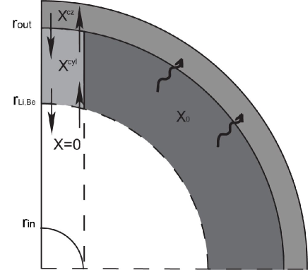
Figure 11: Schematic of the Li (or Be) mass flux in the various regions of a Li-dip star’s interior. The surface and the two radiative–convective interfaces are shown as solid circles. The dashed line represents the Li-burning (or alternatively the Be-burning) radius – only one of the two is shown on this Figure for clarity. Fluid is pumped from the surface downward along the rotation axis, and returns to the outer convection zone in a thin layer close to the edge of the tangent cylinder (vertical dashed line). By mass conservation, both fluxes are the same and equal to $W_{\rm rz}^{\rm spher}\pi r_{\rm in}^{2}$. The mass abundance of Li (and Be) in the outer convection zone is $X^{\rm cz}$, that in the cylinder $C_{\rm Li,Be}$ is $X^{\rm cyl}$ while $X=0$ below the burning radius. In the region below the outer convection zone but above the burning radius, the abundance ($X_{0}$) is essentially primordial. Diffusion (squiggly arrows) brings Li and Be back into the outer convection zone.

Based on the numerical results from §4.1, and best illustrated in Figure 6, we now approximate the Li circulation pattern in the manner depicted in Figure 11 (see also Figure 3). Li-rich fluid is pumped down from the outer convective zone, through the cylindrical region $C_{\rm Li}$ (delimited in radius by the cylinder tangent to the convective core and in the vertical direction by $r_{\rm Li}$ and $r_{\rm out}$ respectively), down to the Li-burning interior. By mass conservation, Li-free material is pumped up from the deep interior, through $C_{\rm Li}$, to the outer convective zone. As a result, $C_{\rm Li}$ and the outer convection zone are both progressively depleted in Li with time.

Note that the timescale for material to flow vertically from the Li-burning radius $r_{\rm Li}$ to the base of the outer convection zone $r_{\rm out}$ (or vice-versa) can easily be calculated by integrating the inverse of the radial velocity $W^{\rm spher}_{\rm rz}/\bar{\rho}$ between $r_{\rm Li}$ and $r_{\rm out}$. The results, using $W^{\rm spher}_{\rm rz}$ estimated above and the true stellar density profiles, are shown in Figure 12, together with the equivalent timescale for the transport of Be from the Be-burning radius $r_{\rm Be}$ to the outer convection zone. In all stars considered, the transport timescales are of the order of 30-100 Myr and 100-300 Myr for Li and Be respectively when the differential rotation rate $a_{2}$ is one percent. Note that the transport timescale is not equal to the depletion timescale, although the two are related (see Appendix B for detail). Figure 12 also shows the similarly calculated timescale required for material to move from the convective core to the convective envelope. It is interesting and reassuring to note that for reasonable values of $a_{2}$, this timescale is of the order of tens of Gyr, so that one would not expect to see a strong modification of the surface abundances of He or CNO nuclei over the lifetime of these stars. This is an important self-consistency check of the model.

Figure 12: Timescales for the circulation of material from the base of the outer convective zone down to the Li-burning radius (solid line), the Be-burning radius (dashed line) and the inner convective core (dotted line). Note that since $W^{\rm spher}_{\rm rz}$ scales linearly with $a_{2}$, so do these timescales, hence the rescaling of the $y-$axis. For reasonable values of $a_{2}$ (of the order of a percent), the Li- and Be-circulation timescales are smaller than the age of the star, while the circulation from the surface down to the inner core is of tens of Gyr.

We now evaluate the rate of change of the mass fraction of Li in the outer convective zone, denoted as $X_{\rm Li}^{\rm cz}$. By definition $X_{\rm Li}^{\rm cz}=M_{\rm Li}^{\rm cz}/M^{\rm out}_{\rm cz}$, the ratio of the total mass of Li in the outer convection zone to the total mass of the outer convection zone. Since material flows through $C_{\rm Li}$ on its way up and down, we also need to define the mass fraction of Li in $C_{\rm Li}$, $X_{\rm Li}^{\rm cyl}=M_{\rm Li}^{\rm cyl}/M(C_{\rm Li})$, i.e. the total mass of Li contained in $C_{\rm Li}$ divided by the mass of that region. Note that

$$M(C_{\rm Li}) = \int_{r_{\rm Li}}^{r_{\rm out}}{\rm d}r\int_{0}^{\sin^{-1}(r_{\rm in}/r)}\quad 2\pi\bar{\rho}(r)r^{2}\sin\theta{\rm d}\theta$$ (37)

$$= \int_{r_{\rm Li}}^{r_{\rm out}}2\pi\bar{\rho}(r)r^{2}\left(1-\sqrt{1-\frac{r_{\rm in}^{2}}{r^{2}}}\right){\rm d}r\mbox{ ,}$$

and can easily be integrated numerically.

Based on Figure 11, we see that

$$\dot{M}^{\rm cz}_{\rm Li}=-\pi r_{\rm in}^{2}W^{\rm spher}_{\rm rz}X^{\rm cz}_{\rm Li}+\pi r_{\rm in}^{2}W^{\rm spher}_{\rm rz}X^{\rm cyl}_{\rm Li}\mbox{ ,}$$

$$\dot{M}^{\rm cyl}_{\rm Li}=\pi r_{\rm in}^{2}W^{\rm spher}_{\rm rz}X^{\rm cz}_{\rm Li}-2\pi r_{\rm in}^{2}W^{\rm spher}_{\rm rz}X^{\rm cyl}_{\rm Li}+0\mbox{ ,}$$ (38)

since the total mass flux both up and down, within the tangent cylinder, is equal to $\pi r_{\rm in}^{2}W^{\rm spher}_{\rm rz}$. Dividing the first equation by $M_{\rm cz}^{\rm out}$ and the second by $M(C_{\rm Li})$, we finally get

$$\dot{X}^{\rm cz}_{\rm Li}=-\frac{\pi r_{\rm in}^{2}W^{\rm spher}_{\rm rz}}{M^{\rm out}_{\rm cz}}X^{\rm cz}_{\rm Li}+\frac{\pi r_{\rm in}^{2}W^{\rm spher}_{\rm rz}}{M^{\rm out}_{\rm cz}}X^{\rm cyl}_{\rm Li}\mbox{ ,}$$

$$\dot{X}^{\rm cyl}_{\rm Li}=\frac{\pi r_{\rm in}^{2}W^{\rm spher}_{\rm rz}}{M(C_{\rm Li})}X^{\rm cz}_{\rm Li}-\frac{2\pi r_{\rm in}^{2}W^{\rm spher}_{\rm rz}}{M(C_{\rm Li})}X^{\rm cyl}_{\rm Li}\mbox{ ,}$$ (39)

which implicitly defines two timescales,

$$\tau^{\rm cz}_{\rm pump}=\frac{M^{\rm out}_{\rm cz}}{\pi r_{\rm in}^{2}W^{\rm spher}_{\rm rz}}\mbox{ ,}$$

$$\tau^{\rm cyl}_{\rm Li,pump}=\frac{M(C_{\rm Li})}{\pi r_{\rm in}^{2}W^{\rm spher}_{\rm rz}}\mbox{ .}$$ (40)

The timescale $\tau^{\rm cz}_{\rm pump}$ is the characteristic timescale over which the material within the outer convection zone is recirculated by gyroscopic pumping, while $\tau^{\rm cyl}_{\rm Li,pump}$ is the timescale over which the material within the cylinder $C_{\rm Li}$ is recirculated. If $\tau^{\rm cz}_{\rm pump}\ll\tau^{\rm cyl}_{\rm Li,pump}$ then $X^{\rm cz}_{\rm Li}\simeq X^{\rm cyl}_{\rm Li}$ at all times. Meanwhile, if $\tau^{\rm cz}_{\rm pump}$ is of the order of or greater than $\tau^{\rm cyl}_{\rm Li,pump}$, then $X^{\rm cz}_{\rm Li}$ can differ from $X^{\rm cyl}_{\rm Li}$ significantly.

The set of equations (39) can easily be solved analytically given the initial condition $X^{\rm cz}_{\rm Li}(t=0)=X^{\rm cyl}_{\rm Li}(t=0)=X_{\rm Li,0}$, the initial Li abundance in the star. The calculation is detailed in Appendix B. A very similar calculation can be done to estimate the surface Be abundance $X^{\rm cz}_{\rm Be}$ as a function of time. The only difference is that one should replace $r_{\rm Li}$ with $r_{\rm Be}$, the Be-burning radius, which defines the slightly larger cylindrical region $C_{\rm Be}$, and equivalently the quantity $X^{\rm cyl}_{\rm Be}$. The timescale $\tau^{\rm cz}_{\rm pump}$ remains the same, while we define

$$\tau^{\rm cyl}_{\rm Be,pump}=\frac{M(C_{\rm Be})}{\pi r_{\rm in}^{2}W^{\rm spher}_{\rm rz}}\mbox{ .}$$ (41)

Our theoretical results, now expressed as Li and Be depletion fractions, are shown in Figure 13, assuming values of $a_{2}=0.002$, $0.005$, and $0.01$. They are compared with observed Li and Be abundances in the Hyades as reported by Boesgaard (2005). It is quite clear that contrary to our naive expectation of §3, the gyroscopic pumping of Li and Be out of the outer convection zone does not decrease for the higher-mass stars despite the fact that their outer convection zone becomes smaller and smaller. This is also clear from Figure 10, where $W_{\rm rz}^{\rm spher}$ continues to increase with stellar mass instead of being quenched as initially expected. In the next sections, we discuss why this is the case, and how to reconcile the model with observations.

Figure 13: Relative depletion of Li and Be in the Hyades cluster (assumed to be 700Myr old) as a function of stellar mass around the Li dip. Note that $\Delta N({\rm Li})=\log(X_{\rm Li}^{\rm cz}/X_{\rm Li,0})$ and similarly for Be. The thin lines connecting the symbols show data interpolated from Boesgaard (2005). The solid line and squares correspond to the Li data, while the dashed lines and triangle correspond to the Be data. The model predictions are shown in thick solid and dashed lines for the Li and Be cases respectively, from top to bottom in each case for $a_{2}=0.002$, $0.005$ and $0.01$ (the larger $a_{2}$, the larger the depletion).

5.2.3 Discussion

The most important conclusion from this analysis is that gyroscopic pumping alone may be able to explain the cool side of the dip for reasonable values of the differential rotation rate (one merely needs to adjust $a_{2}$), but always vastly over-estimates the depletion rate for stars on the hot side of the dip. Since the gyroscopic pumping mechanism is quite generic, and arises from simple first-principles of angular momentum conservation our study then raises the question of how one might suppress the effects of pumping in the hot side of the dip. In order to address the problem, it is important first to understand the cause of the sharp decrease in the predicted depletion timescale for high-mass stars in this model.

First, note that most of the pumping in the stars considered comes from the inner core. Indeed, the density in the outer convection zone is so low that the mass flux $\bar{\rho}u_{\rm cz}^{\rm out}$ generated in the outer convection zone is negligible compared with the mass flux generated from the inner convection zone (see equation (19)). As a result, the characteristics of the inner core dominate the forcing of the flows, while the outer convection zone merely plays the role of providing a pathway for the flows to return to the interior. This is easily verified numerically by setting (artificially) $\Lambda_{\rm out}=0$ to suppress the forcing in the outer convection zone. Since turbulent viscosity in the outer convection zone is nevertheless still present, the return path still exists and as seen in Figure 14, the resulting depletion rates are hardly changed.

One may then wonder what the main factor controlling the variation in the depletion rate as a function of stellar mass actually is. A few immediate possibilities come to mind. The convective velocities in the inner core of these stars, as well as the size of the inner core (see Table 1), both increase with $M_{\star}$, implying that the total mass flux pumped by the inner convection zone is larger for stars on the hot side of the dip. In addition, the increase in the rotation rates of the stars as $M_{\star}$ increases implies that the allowed flow speeds through the radiative zone are larger on the hot side of the dip (see equation (24)). All of these effects explain the trend seen in Figure 10, which clearly shows that the pumped mass flux $W_{\rm rz}^{\rm spher}$ increases with $M_{\star}$ across the dip.

However, this is not sufficient to explain the vast increase in the depletion rates observed in Figure 13 as $M_{\star}$ increases. In Figure 14 we show different artificial models to illustrate this statement. Model M1 is the aforementioned case where $\Lambda_{\rm out}$ is set to zero. Model M2 is created holding $\Omega_{\star}$ constant and equal to $10^{-4}$rad/s across all stars in the model, to suppress the effect of increased rotation rate across the dip. Model M3 is created holding $\Lambda_{\rm in}$ constant and equal to 10 across all stars in the model, to suppress the effect of increased convective velocities across the dip. Model M4 is created holding $r_{\rm in}$ constant and equal to 0.05$R_{\star}$ across all stars in the model, to suppress the effect of increased core size across the dip. In all cases, all other quantities are the same as the original model of Figure 13. As we can see, none of these changes affect the predicted depletion rates much. This incidentally also shows that the exact details of the model are not particularly important, and that another, much more fundamental effect controls the overall depletion rate. Finally, we show (as the two dotted lines) a variant of model M2 in which $\Omega_{\star}$ is held constant but this time equal to $2\times 10^{-5}$rad/s. This value is closer to the typical angular velocity (derived from $v\sin i$) of stars for which Li has actually been observed, which is significantly smaller than the median rotation rates for stars of the same mass (see Boesgaard 1987). Very similar depletion rates to those of models M1-M4 can be recovered provided the overall differential rotation is chosen to be larger ($a_{2}=0.08$). This shows that there is some degeneracy in the model parameters, which is not entirely surprising.

Figure 14: Relative depletion of Li (solid lines) and Be (dashed lines) in the Hyades cluster as a function of stellar mass in the Li dip, as predicted in various artificial test-models. $\Delta N$ is defined as in Fig. 13. In all cases, $a_{2}=0.002$. In model M1, $\Lambda_{\rm out}$ is set to zero for all stars. In model M2, $\Omega_{\star}=10^{-4}$rad/s for all stars. The dotted lines show the variant of model M2 for which $\Omega_{\star}=2\times 10^{-5}$rad/s and $a_{2}=0.08$, for Li and Be respectively. In model M3, $\Lambda_{\rm in}=10$ for all stars. In model M4, $r_{\rm in}=0.05R_{\star}$ for all stars. In model M5, the mass of the outer convective zone is set $10^{-3}M_{\odot}$ for all stars. In model M6, the contribution of the cylinder (see main text) to $M_{\rm Li}$ and $M_{\rm Be}$ is set to 0. All other quantities are as in Figure 13. Note that in model M6, the two lines for Li and Be are on top of each other, as expected from the analytical model.

The dominant effect in the model depletion trend is in fact found to be the decrease in the mass of the regions which need to be depleted in Li or Be as $M_{\star}$ increases. This mass has two contributions: the mass of the outer convective zone $M_{\rm out}^{\rm cz}$, plus the mass contained in the cylinders $C_{\rm Li}$ and $C_{\rm Be}$ respectively. To illustrate the effect in question, we create two additional artificial models. In model M5 the mass of the outer convective zone is artificially held constant (and equal to $10^{-3}M_{\odot}$). In model M6 the mass in the cylinders is set to 0 (assuming that only the Li and Be fractions in the convective zone need to be recirculated). The results are also shown in Figure 14. The depletion rates in each case are now strikingly different from those of models M1-4. In the case of M5, the depletion fraction is now much more constant across all stars. This strongly suggests that the depletion timescale in Figure 13 varies with stellar mass more because the total mass which needs to be depleted varies than because the pumped mass flux $W_{\rm rz}^{\rm spher}$ varies. Model M6 illustrates a fundamental property of these rapidly rotating Li-dip stars undergoing gyroscopic pumping. Since the pumped mass flux is independent of depth below the convection zone, unless the mass of Be to be depleted is different from the mass of Li to be depleted, the predicted depletion timescales will be exactly the same for the two species. This is precisely the case illustrated by model M6 which ignores the contribution of the cylinders $C_{\rm Li}$ and $C_{\rm Be}$, so the predicted depletion fractions of Li and Be are exactly the same. Hence, the mixed inner cylinders are crucial to the difference in the depletion timescales of Li and Be. Moreover, their radii and heights uniquely determine the predicted ratio of the Li and Be depletion fraction. As seen in Figure 13, the original model described in §5.2.2 appears to predict the correct ratio, even though the absolute depletion fractions are too large for the hot side of the dip.

The remaining question is why the pumping is not suppressed for stars of masses higher than 1.5$M_{\odot}$, as originally expected from the gradual disappearance of the outer convective zone. In fact, it turns out that $d_{\rm out}$ and $v_{\rm conv}^{\rm out}$ remain significant in these stars, even though the total mass of the convection zone becomes negligible. Since the main role of the outer convection zone is to provide a pathway to recirculate the small mass flux pumped by the inner core, there is no notable suppression of the pumping in this mass range contrary to our original idea described in §3.

5.3 The role of Li (and Be) diffusion

While the model as it stands appears to reproduce the depletion trend on the cool side of the dip with reasonable assumptions for the differential rotation of the inner core ($a_{2}=O(0.01)$), it vastly overestimates the depletion fraction on the hot side of the dip. Our efforts now shift to the problem of reconciling the model with observations, or in other words on reducing the depletion rate on the hot side of the dip.

The answer, as it happens, is quite simple, and lies in the balance between advection of Li-rich (and Be-rich) material out of the outer convection zone by gyroscopic pumping, and diffusion of these elements back into it from the radiative zone below which, as illustrated in Figure 11, still has primordial Li and Be abundances. To take this new effect into account, equation (38) must be modified as

$$\dot{M}^{\rm cz}_{\rm Li}=-\pi r_{\rm in}^{2}W^{\rm spher}_{\rm rz}X^{\rm cz}_{\rm Li}+\pi r_{\rm in}^{2}W^{\rm spher}_{\rm rz}X^{\rm cyl}_{\rm Li}-4\pi r_{\rm out}^{2}\bar{\rho}(r_{\rm out})D\nabla X_{\rm Li}\mbox{ ,}\\$$

where the new third term is the mass flux of Li diffused back into the outer convection zone. The diffusion coefficient $D$ is presumably the sum of a microscopic and a turbulent contribution from convective overshoot. The microscopic contribution is evaluated using the prescription of Gough (2007), while the turbulent contribution presumably decays exponentially with depth below the convection zone on a typical overshoot depth lengthscale, yielding

$$D(r)=D_{\rm micro}(r)+D_{\rm turb}(r)=D_{\rm micro}(r)+v_{\rm conv}^{\rm out}d_{\rm out}\exp\left(\frac{r-r_{\rm out}}{\Delta_{\rm out}}\right)\mbox{ for }r<r_{\rm out}\,.$$ (42)

The equation for the evolution of $M_{\rm Li}^{\rm cyl}$ remains unchanged (neglecting the diffusion of Li through the sides of the cylinder for simplicity).

Unfortunately, the addition of a diffusive component to the Li flux now prevents us from deriving simple analytical solutions of these equations analogous to the ones found in §5.2.2. Instead, solutions can only be obtained numerically by integrating the partial differential equation (5.3) with time, and following the evolution of the spatially varying Li profile. Given the other approximations made throughout this work (e.g. assuming that the rotation rate of the star, the background stellar structure and the convective forcing are all constant with time), and since our aim is merely a preliminary “proof-of-concept”, it seems futile to try to obtain a precise numerical solution of (5.3).

Instead, in this first paper we proceed by approximating the gradient term to cast (5.3) in the form of an ordinary differential equation similar to (39). This can be done simply be writing

$$\nabla X_{\rm Li}=\frac{X_{\rm Li}^{\rm cz}-X_{\rm Li,0}}{d_{\rm diff}}\mbox{ ,}$$ (43)

where we have assumed that there is a “reservoir” of material with primordial Li abundance in the radiative zone in the form of a spherical shell of width $d_{\rm diff}$ adjacent to $r_{\rm out}$, and that Li has to diffuse across that reservoir to be mixed into the convection zone. For this reservoir to contain enough Li to replenish the convection zone it must have roughly the same mass, so we set $d_{\rm diff}=\beta d_{\rm out}$ where $\beta$ is a free parameter of the problem of order unity. Finally, the diffusion coefficient must also be approximated by a constant for (5.3) to become a true ODE. Since the turbulent transport is weakest furthest from the radiative–convective interface, this is the “bottleneck” region for the diffusion of Li back into the convection zone. Hence we take

$$D=D_{\rm micro}(r_{\rm out}-d_{\rm diff})+v_{\rm conv}^{\rm out}d_{\rm out}\exp\left(-\frac{d_{\rm diff}}{\Delta_{\rm out}}\right)\mbox{ .}$$ (44)

As before, we divide (5.3) by $M_{\rm cz}^{\rm out}$ to get

$$\dot{X}^{\rm cz}_{\rm Li}\simeq-\frac{X^{\rm cz}_{\rm Li}}{\tau^{\rm cz}_{\rm pump}}+\frac{X^{\rm cyl}_{\rm Li}}{\tau^{\rm cz}_{\rm pump}}-\frac{X_{\rm Li}^{\rm cz}-X_{\rm Li}(0)}{\tau_{\rm diff}}\mbox{ ,}$$

$$\dot{X}^{\rm cyl}_{\rm Li}\simeq\frac{X^{\rm cz}_{\rm Li}}{\tau^{\rm cyl}_{\rm Li,pump}}-2\frac{X^{\rm cyl}_{\rm Li}}{\tau^{\rm cyl}_{\rm Li,pump}}\mbox{ ,}$$ (45)

where

$$\tau_{\rm diff}=\frac{D}{d_{\rm diff}d_{\rm out}}\frac{4\pi r_{\rm out}^{2}d_{\rm out}\bar{\rho}(r_{\rm out})}{M_{\rm cz}^{\rm out}}\simeq\frac{D}{\beta d_{\rm out}^{2}}\mbox{ .}$$ (46)

As shown in Appendix B, one can integrate these equations analytically fairly straightforwardly. We find, as expected on physical grounds, that when the Li diffusion timescale into the convection zone becomes shorter than the advection timescale out of the convection zone, the surface Li abundance remains close to the primordial value.

The resulting depletion fractions calculated using this method, for Li and Be, are shown in Fig. 15 for a simple grid of parameters ($a_{2}=0.005$, $a_{2}=0.02$, $\beta=0.9$ and $\beta=1.1$), with the stellar models otherwise exactly the same as the ones used to create Figure 13. Note how, for all chosen parameter values, the Li and Be profiles now exhibit a clear dip centered roughly around the position of the observed Li-dip. On the cool side the effects of diffusion are negligible and the predicted depletion rates are very similar to the ones obtained in the absence of diffusion (see Figure 13). On the hot side, diffusion is important and continuously replenishes the outer convection zone with Li-rich and Be-rich material. The transition between the cool and hot sides, in the model, occurs when the diffusion timescale of Li back into the convection zone, namely $\tau_{\rm diff}$, becomes comparable with the advection timescale of Li-rich material out of it (namely $\tau^{\rm cz}_{\rm Li,pump}$), and depends both on the diffusion rate (as controlled by $\beta$ for example) and on the pumping rate (as controlled by $a_{2}$).

Note that for the larger value of $a_{2}$, the ratio of the Li depletion fraction to the Be depletion fraction within the dip remains close to 1, contrary to observations. Instead, the ratio of the predicted depletion fractions is closer to observations for lower values of $a_{2}$. The overall “best fit” is found for $a_{2}=0.005$ and $\beta=0.9$, which are not unreasonable parameter values. However, with our very crude model of the diffusion, we are not able to fit the exact position and amplitude of both Li and Be dips simultaneously. Since we were only aiming for a proof-of-concept, we view the results obtained as quite satisfactory, although a more careful model will be required in the future should one wish to explain the structure of both dips in more detail.

Figure 15: Relative depletion of Li (solid lines) and Be (dashed lines) in the Hyades cluster as a function of stellar mass in the Li dip, as predicted for various values of the model parameters $a_{2}$ (related to the stellar differential rotation) and $\beta$ (related to the diffusion of chemical species across the base of the convection zone). $\Delta N$ is defined as in Fig. 13. See main text for detail.

5.4 Summary

To summarize this section, we have found that the combination of gyroscopic pumping and turbulent diffusion of chemical species by overshooting motions ubiquitously predicts the presence of a dip in both Li and Be surface abundances for young MS stars in the mass range $1.3-1.5M_{\odot}$ (Li-dip stars). Depletion profiles close to the observed ones can be reproduced for reasonable values of model parameters. The increase in the depletion fraction on the cool side of the dip is explained by gyroscopic pumping and the progressively smaller amount of material which needs to be recirculated, while the decrease in the depletion fraction on the hot side of the dip is explained by the effect of diffusion on replenishing the outer convection zone with Li and Be.

6 Discussion and prospects

In this paper we performed an exhaustive study of a non-local source of rotational mixing called “gyroscopic pumping”, which was originally studied in the context of the Earth’s atmosphere by Haynes et al. (1991) and later discussed in the case of the Sun by Gough & McIntyre (1998), McIntyre (2007), and GAA09.

In this mechanism, large-scale meridional motions are driven by angular-momentum conservation whenever fluid undergoes forces in the azimuthal direction (see §1.2 and in particular Figure 1 for detail). This is exactly the case in stellar convective zones, where rotationally influenced convection gives rise to the so-called $\Lambda-$effect (cf. Rüdiger 1989; see also Garaud et al. 2010), and typically leads to the azimuthal acceleration of equatorial regions and deceleration of the poles. The resulting large-scale meridional circulation has fluid flowing outward from the rotation axis near the equator, and toward the rotation axis near the pole. Note that this mechanism is quite generic, since it is simply based on angular momentum conservation. However, by contrast with other well-studied significant sources of rotational mixing, it does not rely on stellar spin-down to be effective – it is an inherently quasi-steady mechanism.

As first shown by GAA09 and studied more extensively here, whether the fluid gyroscopically pumped in the convective zone ends up mixing the nearby radiative zone or not depends on many factors. The case of stars with a single convection zone, in the absence of any other mechanism, was first studied by GAA09. In this case the overall amplitude of the flows penetrating into the radiative zone is limited to slow Ekman flows, which are unlikely to play any significant role in mixing the stellar interior. However, this conclusion could be different if a large-scale magnetic field is present (Gough & McIntyre 1998), as it is for instance thought to be the case in the Sun. We defer the magnetic case to a subsequent paper.

Here we focused on stars with two convection zones, in the absence of magnetic fields (we accept that this approximation is probably over-simplistic). We found that gyroscopic pumping provides a significant source of non-local mixing in the radiative zones of these stars, more precisely along the rotation axis, within the cylinder tangent to the inner core (see Figure 11). This mixing readily explains, for example, the cool side of the well-known Li-dip and, when moderated by the effects of diffusion, provides predictions for the Li- and Be-depletion fractions which give a surprisingly good fit to the data on both sides of the dip (see Figure 15). It is important to note that contrary to previous models, turbulent mixing here is needed not to explain Li destruction but to explain the replenishment of the surface layers in Li. Of course, the various other effects described in §5.1, which were not taken into account here, could also affect the Li and Be abundances: mixing by gravity waves, large-scale rotational mixing induced by stellar spin-down, radiative acceleration, etc. A more sophisticated study of the Li-dip in the light of gyroscopic pumping, taking these effects into account as well as stellar evolution, is deferred to a subsequent publication. Furthermore, it is interesting to note that the gyroscopic pumping mechanism probably plays a role in the global redistribution of angular momentum within the star. Whether this is related to the dichotomy between slow rotators and fast rotators on either side of the dip is an interesting question, which we hope to address in the future.

Gyroscopic pumping, as studied here, also opens up other interesting observational prospects beyond Li-dip stars. For example, another important evolutionary phase when stars have two convective zones is the core helium burning phase on the red giant branch. Our study shows that this pumping mechanism could provide an important connection between the convective envelope and the core, and perhaps help reconciliate some of the long-standing discrepancies in surface abundances of CNO elements between models and observations. It is also interesting to note that the pumping itself has a tendency to drive a strong azimuthal shear in the system, close to the tangent cylinder (see Figure 6). This shear could perhaps become unstable for very rapidly rotating stars, leading to much more violent mixing in the radiative zone. Alternatively, this shear layer could also become the seat of an $\Omega-$effect and generate strong toroidal fields around the tangent cylinder. It is interesting to speculate on what kind of field such a flow structure would sustain, and what observable feature it may lead to – although a full answer to that question will require a study of gyroscopic pumping in the presence of magnetic fields.

Appendix A: Analytical derivation of $W_{\rm rz}$

In this appendix, we derive the analytical expression for the solution of the Cartesian model described in §3.2.1, focusing in particular on the derivation of the mass flux into the radiative zone, $W_{\rm rz}$. Solutions to the set of equations (16) are first found in each of the three regions separately, then matched to one another at the interfaces (at $z_{\rm in}$ and $z_{\rm out}$) and to boundary conditions (at $z=0$ and $z=1$).

Solution in the outer convection zone.

In the outer convection zone, the viscous stresses are negligible compared with the linear drag term and $N(z)=0$. As a result, the equations reduce to

$$\hat{T}_{zz}-k^{2}\hat{T}=0\mbox{ , }$$

$$-2\hat{v}=-\Lambda_{\rm out}(\hat{u}-\hat{u}^{\rm out}_{\rm cz})\mbox{ , }$$

$$2\hat{u}=-ike^{z/D_{\rho}}\hat{p}-\Lambda_{\rm out}\hat{v}\mbox{ , }$$

$$0=-\hat{p}_{z}e^{z/D_{\rho}}+e^{z/D_{T}}\hat{T}-\Lambda_{\rm out}\hat{w}\mbox{ , }$$

$$e^{-z/D_{\rho}}ik\hat{v}+(e^{-z/D_{\rho}}\hat{w})_{z}=0\mbox{ . }$$ (47)

The temperature equation is easily solved as

$$\hat{T}(z)=ae^{kz}+be^{-kz}\mbox{ . }$$ (48)

The remaining system of four equations can by transformed into a linear system of ODEs with constant coefficients using the following new mass flux variables: $U=e^{-z/D_{\rho}}\hat{u}$ (and similarly for $u_{\rm cz}$), $V=e^{-z/D_{\rho}}\hat{v}$, and $W=e^{-z/D_{\rho}}\hat{w}$. In that case,

$$-2V=-\Lambda_{\rm out}(U-U^{\rm out}_{\rm cz})\mbox{ , }$$

$$2U=-ik\hat{p}-\Lambda_{\rm out}V\mbox{ , }$$

$$0=-\hat{p}_{z}-\Lambda_{\rm out}W+Te^{-z/L}\mbox{ , }$$

$$ikV+W_{z}=0\mbox{ , }$$ (49)

where $L^{-1}=D_{\rho}^{-1}-D_{T}^{-1}$.

Eliminating each variable in turn we can reduce the system to a second-order, forced linear ordinary differential equation for $W$ (for example):

$$W_{zz}=W\frac{k^{2}\Lambda_{\rm out}^{2}}{4+\Lambda_{\rm out}^{2}}+\frac{2ik\Lambda_{\rm out}}{4+\Lambda_{\rm out}^{2}}S_{\rm cz}^{\rm out}-e^{-z/L}\frac{k^{2}\Lambda_{\rm out}}{4+\Lambda_{\rm out}^{2}}\hat{T}\mbox{ ,}$$ (50)

where

$$S_{\rm cz}^{\rm out}(z)=\frac{{\rm d}U^{\rm out}_{\rm cz}(z)}{{\rm d}z}=\frac{{\rm d}}{{\rm d}z}\left(e^{-z/D_{\rho}}\hat{u}^{\rm out}_{\rm cz}(z)\right)\mbox{ .}$$ (51)

The solution of this equation is the sum of the solution of the homogeneous problem plus a particular solution. If we assume for simplicity that $S_{\rm cz}^{\rm out}$ is constant in the outer convection zone , the particular solution is easily expressed as:

$$W(z)=Ae^{z/\delta_{\rm out}}+Be^{-z/\delta_{\rm out}}-\frac{2iS_{\rm cz}^{\rm out}}{k\Lambda_{\rm out}}-\frac{a}{\Lambda_{\rm out}}\frac{e^{(k-L^{-1})z}}{\delta_{\rm out}^{2}(k-L^{-1})^{2}-1}-\frac{b}{\Lambda_{\rm out}}\frac{e^{(-k-L^{-1})z}}{\delta_{\rm out}^{2}(k+L^{-1})^{2}-1}\mbox{ ,}$$ (52)

where we have defined the new lengthscale

$$\delta_{\rm out}=\frac{\sqrt{4+\Lambda_{\rm out}^{2}}}{k\Lambda_{\rm out}}\mbox{ .}$$ (53)

Using the solutions obtained for $W$ and $T$ we deduce the solution for the pressure perturbation:

$$\hat{p}(z) = \frac{2iU^{\rm out}_{\rm cz}}{k}-\Lambda_{\rm out}\delta_{\rm out}\left(Ae^{z/\delta_{\rm out}}-Be^{-z/\delta_{\rm out}}\right)$$ (54)

$$+ a\frac{(k-L^{-1})e^{(k-L^{-1})z}}{(k-L^{-1})^{2}-\delta_{\rm out}^{-2}}-b\frac{(k+L^{-1})e^{(-k-L^{-1})z}}{(k+L^{-1})^{2}-\delta_{\rm out}^{-2}}\mbox{ .}$$

Solution in the inner convection zone.

By analogy, the solutions in the inner convection zone are given by

$$\hat{T}(z)=ce^{kz}+de^{-kz}$$

$$W(z)=Ce^{z/\delta_{\rm in}}+De^{-z/\delta_{\rm in}}-\frac{2iS_{\rm cz}^{\rm in}}{k\Lambda_{\rm in}}-\frac{c}{\Lambda_{\rm in}}\frac{e^{(k-L^{-1})z}}{\delta_{\rm in}^{2}(k-L^{-1})^{2}-1}-\frac{d}{\Lambda_{\rm in}}\frac{e^{(-k-L^{-1})z}}{\delta_{\rm in}^{2}(k+L^{-1})^{2}-1}\mbox{ ,}$$

$$\hat{p}(z)=\frac{2iU^{\rm in}_{\rm cz}}{k}-\Lambda_{\rm in}\delta_{\rm in}\left(Ce^{z/\delta_{\rm in}}-De^{-z/\delta_{\rm in}}\right)$$

$$\quad\quad\quad+c\frac{(k-L^{-1})e^{(k-L^{-1})z}}{(k-L^{-1})^{2}-\delta_{\rm in}^{-2}}-d\frac{(k+L^{-1})e^{(-k-L^{-1})z}}{(k+L^{-1})^{2}-\delta_{\rm in}^{-2}}\mbox{ ,}$$ (55)

where $\delta_{\rm in}$ and $S_{\rm cz}^{\rm in}$ are defined by analogy with $\delta_{\rm out}$ and $S_{\rm cz}^{\rm out}$ and where four new integration constants ($c$, $d$, $C$ and $D$) have been introduced.

Solution in the radiative zone.

In the radiative zone, the governing equations (16) reduce to

$$-2\hat{v}=E_{\nu}\left(\hat{u}_{zz}-k^{2}\hat{u}\right)\mbox{ , }$$

$$2\hat{u}=-ik\hat{p}e^{z/D_{\rho}}+E_{\nu}\left(\hat{v}_{zz}-k^{2}\hat{v}\right)\mbox{ , }$$

$$0=-\hat{p}_{z}e^{z/D_{\rho}}+\hat{T}e^{z/D_{T}}+E_{\nu}\left(\hat{w}_{zz}-k^{2}\hat{w}\right)\mbox{ , }$$

$$\frac{N_{\rm rz}^{2}}{\Omega_{\star}^{2}}e^{-z/D_{T}}\hat{w}=E_{\kappa}\left(\hat{T}_{zz}-k^{2}\hat{T}\right)\mbox{ , }$$

$$ik\hat{v}e^{-z/D_{\rho}}+(e^{-z/D_{\rho}}\hat{w})_{z}=0\mbox{ . }$$ (56)

In the limit of very small Ekman number, and for $\sigma<1$, the system is approximated by

$$-2\hat{v}=O(E_{\nu})\mbox{ , }$$

$$2\hat{u}=-ike^{z/D_{\rho}}\hat{p}+O(E_{\nu})\mbox{ , }$$

$$e^{z/D_{\rho}}\hat{p}_{z}=e^{z/D_{T}}\hat{T}+O(E_{\nu})\mbox{ , }$$

$$e^{-z/D_{T}}\frac{N_{\rm rz}^{2}}{\Omega_{\star}^{2}}\hat{w}=E_{\kappa}(\hat{T}_{zz}-k^{2}\hat{T})\mbox{ , }$$

$$(e^{-z/D_{\rho}}\hat{w})_{z}=O(E_{\nu})\mbox{ , }$$ (57)

which successively implies that

$$e^{-z/D_{\rho}}\hat{w}=W_{\rm rz}+O(E_{\nu})\mbox{ , }$$

$$\hat{T}=K_{1}e^{kz}+K_{2}e^{-kz}+\frac{N_{\rm rz}^{2}}{\Omega_{\star}^{2}}\frac{W_{\rm rz}}{E_{\kappa}}\frac{e^{z/L}}{L^{-2}-k^{2}}+O(E_{\nu})\mbox{ , }$$

$$\hat{p}=p_{\rm rz}+\frac{K_{1}e^{z(k-L^{-1})}}{k-L^{-1}}-\frac{K_{2}e^{z(-k-L^{-1})}}{k+L^{-1}}+\frac{N_{\rm rz}^{2}}{\Omega_{\star}^{2}}\frac{W_{\rm rz}}{E_{\kappa}}\frac{z}{L^{-2}-k^{2}}+O(E_{\nu})\mbox{ , }$$ (58)

and where $W_{\rm rz}$, $K_{1}$, $K_{2}$ and $p_{\rm rz}$ are integration constants.

We see that the condition where $\bar{\rho}\hat{w}$ is constant arises simply from mass conservation and geostrophy. Assuming that $W_{\rm rz}$ is known, the pumped flow induces local temperature perturbations as a result of the thermal energy equation: this can easily be seen in the solution for $\hat{T}$, which contains two parts: the particular solution of the Poisson problem which includes the source term arising from the advection of the background temperature by the meridional flows, plus the general solution of $\nabla^{2}\hat{T}=0$. The constants $K_{1}$ and $K_{2}$ are simply there to match the temperature profile in the radiative zone to that of the convection zones. The expression for the pressure perturbation can be interpreted in a similar way.

Matching the solutions and radial velocity in the radiative zone.

We have found twelve integration constants, which can be uniquely determined by applying four boundary conditions (impermeability at $z=0$ and $z=1$, and $\hat{T}=0$ at the top and the bottom) and eight matching conditions (continuity of $\hat{w}$ – alternatively of $W$ – $\hat{p}$, $\hat{T}$ and $d\hat{T}/dz$ at each of the two interfaces).

The boundary conditions at $z=0$ and $z=1$ imply:

$$Ae^{1/\delta_{\rm out}}+Be^{-1/\delta_{\rm out}}=\frac{2iS_{\rm cz}^{\rm out}}{k\Lambda_{\rm out}}+\frac{a}{\Lambda_{\rm out}}\frac{e^{(k-L^{-1})}}{\delta_{\rm out}^{2}(k-L^{-1})^{2}-1}+\frac{b}{\Lambda_{\rm out}}\frac{e^{(-k-L^{-1})}}{\delta_{\rm out}^{2}(k+L^{-1})^{2}-1}\mbox{ , }$$

$$C+D=\frac{2iS_{\rm cz}^{\rm in}}{k\Lambda_{\rm in}}+\frac{c}{\Lambda_{\rm in}}\frac{1}{\delta_{\rm in}^{2}(k-L^{-1})^{2}-1}+\frac{d}{\Lambda_{\rm in}}\frac{1}{\delta_{\rm in}^{2}(k+L^{-1})^{2}-1}\mbox{ , }$$

$$ae^{k}+be^{-k}=0\mbox{ , }$$

$$c+d=0\mbox{ . }$$ (59)

Continuity of vertical velocity, pressure, temperature and derivative of temperature at the $z=z_{\rm out}$ interface implies

$$Ae^{z_{\rm out}/\delta_{\rm out}}+Be^{-z_{\rm out}/\delta_{\rm out}}-\frac{2iS_{\rm cz}^{\rm out}}{k\Lambda_{\rm out}}-\frac{a}{\Lambda_{\rm out}}\frac{e^{(k-L^{-1})z_{\rm out}}}{\delta_{\rm out}^{2}(k-L^{-1})^{2}-1}-\frac{b}{\Lambda_{\rm out}}\frac{e^{(-k-L^{-1})z_{\rm out}}}{\delta_{\rm out}^{2}(k+L^{-1})^{2}-1}=W_{\rm rz}\mbox{ , }$$

$$\frac{2iU^{\rm out}_{\rm cz}}{k}-\delta_{\rm out}\Lambda_{\rm out}\left[Ae^{z_{\rm out}/\delta_{\rm out}}-Be^{-z_{\rm out}/\delta_{\rm out}}\right]+a\frac{(k-L^{-1})e^{(k-L^{-1})z_{\rm out}}}{(k-L^{-1})^{2}-\delta_{\rm out}^{-2}}-b\frac{(k+L^{-1})e^{(-k-L^{-1})z_{\rm out}}}{(k+L^{-1})^{2}-\delta_{\rm out}^{-2}}$$

$$\quad\quad\quad\quad=p_{\rm rz}+\frac{K_{1}e^{z_{\rm out}(k-L^{-1})}}{k-L^{-1}}-\frac{K_{2}e^{z_{\rm out}(-k-L^{-1})}}{k+L^{-1}}+\frac{N_{\rm rz}^{2}}{\Omega_{\star}^{2}}\frac{W_{\rm rz}}{E_{\kappa}}\frac{z_{\rm out}}{L^{-2}-k^{2}}\mbox{ , }$$

$$ae^{kz_{\rm out}}+be^{-kz_{\rm out}}=K_{1}e^{kz_{\rm out}}+K_{2}e^{-kz_{\rm out}}+\frac{N_{\rm rz}^{2}}{\Omega_{\star}^{2}}\frac{W_{\rm rz}}{E_{\kappa}}\frac{e^{z_{\rm out}/L}}{L^{-2}-k^{2}}\mbox{ , }$$

$$kae^{kz_{\rm out}}-kbe^{-kz_{\rm out}}=kK_{1}e^{kz_{\rm out}}-kK_{2}e^{-kz_{\rm out}}+\frac{N_{\rm rz}^{2}}{\Omega_{\star}^{2}}\frac{W_{\rm rz}}{LE_{\kappa}}\frac{e^{z_{\rm out}/L}}{L^{-2}-k^{2}}\mbox{ . }$$ (60)

Similar matching conditions at the lower interface ($z=z_{\rm in}$) imply

$$Ce^{z_{\rm in}/\delta_{\rm in}}+De^{-z_{\rm in}/\delta_{\rm in}}-\frac{2iS_{\rm in}}{k\Lambda_{\rm in}}-\frac{c}{\Lambda_{\rm in}}\frac{e^{(k-L^{-1})z_{\rm in}}}{\delta_{\rm in}^{2}(k-L^{-1})^{2}-1}-\frac{d}{\Lambda_{\rm in}}\frac{e^{(-k-L^{-1})z_{\rm in}}}{\delta_{\rm in}^{2}(k+L^{-1})^{2}-1}=W_{\rm rz}\mbox{ , }$$

$$\frac{2iU^{\rm in}_{\rm cz}}{k}-\delta_{\rm in}\Lambda_{\rm in}\left[Ce^{z_{\rm in}/\delta_{\rm in}}-De^{-z_{\rm in}/\delta_{\rm in}}\right]+c\frac{(k-L^{-1})e^{(k-L^{-1})z_{\rm in}}}{(k-L^{-1})^{2}-\delta_{\rm in}^{-2}}-d\frac{(k+L^{-1})e^{(-k-L^{-1})z_{\rm in}}}{(k+L^{-1})^{2}-\delta_{\rm in}^{-2}}$$

$$\quad\quad\quad\quad=p_{\rm rz}+\frac{K_{1}e^{z_{\rm im}(k-L^{-1})}}{k-L^{-1}}-\frac{K_{2}e^{z_{\rm in}(-k-L^{-1})}}{k+L^{-1}}+\frac{N_{\rm rz}^{2}}{\Omega_{\star}^{2}}\frac{W_{\rm rz}}{E_{\kappa}}\frac{z_{\rm in}}{L^{-2}-k^{2}}\mbox{ , }$$

$$ce^{kz_{\rm in}}+de^{-kz_{\rm in}}=K_{1}e^{kz_{\rm in}}+K_{2}e^{-kz_{\rm in}}+\frac{N_{\rm rz}^{2}}{\Omega_{\star}^{2}}\frac{W_{\rm rz}}{E_{\kappa}}\frac{e^{z_{\rm in}/L}}{L^{-2}-k^{2}}\mbox{ , }$$

$$kce^{kz_{\rm in}}-kde^{-kz_{\rm in}}=kK_{1}e^{kz_{\rm in}}-kK_{2}e^{-kz_{\rm in}}+\frac{N_{\rm rz}^{2}}{\Omega_{\star}^{2}}\frac{W_{\rm rz}}{LE_{\kappa}}\frac{e^{z_{\rm in}/L}}{L^{-2}-k^{2}}\mbox{ .}$$ (61)

This system of twelve equations can in principle be solved analytically exactly, but the solutions are horrendously complicated and without much interest. To get a better physical intuition of the solutions, we restrict our study to stars where the convection zone depths $d_{\rm in}$ and $d_{\rm out}$ are small compared with $k$, $\delta_{\rm in}$ and $\delta_{\rm out}$. Since $k=2$, and $\delta_{\rm in}$ and $\delta_{\rm out}$ are always greater than one for all possible value of $\Lambda_{\rm in}$ and $\Lambda_{\rm out}$, it is sufficient to require that $d_{\rm in}$ and $d_{\rm out}$ be much smaller than one. Note that the $d_{\rm in}\ll 1$ and $d_{\rm out}\ll 1$ approximations are acceptable for all Li-dip stars, which have thin outer convective regions and small convective cores. We also note that $L$ is typically small compared with $\delta$ or $1/k$, although could be of the same order of magnitude as $d_{\rm in}$ and $d_{\rm out}$.

We begin by solving for the constants $a$, $b$, $c$, $d$, $K_{1}$ and $K_{2}$ in terms of $W_{\rm rz}$. This yields, in the limit of thin convection zones:

$$a=K_{1}+\frac{N_{\rm rz}^{2}}{2\Omega_{\star}^{2}}\frac{W_{\rm rz}L^{2}}{E_{\kappa}}e^{z_{\rm out}/L}e^{-kz_{\rm out}}\left(1+\frac{1}{kL}\right)\mbox{ , }$$

$$b=K_{2}+\frac{N_{\rm rz}^{2}}{2\Omega_{\star}^{2}}\frac{W_{\rm rz}L^{2}}{E_{\kappa}}e^{z_{\rm out}/L}e^{kz_{\rm out}}\left(1-\frac{1}{kL}\right)\mbox{ , }$$

$$c=K_{1}+\frac{N_{\rm rz}^{2}}{2\Omega_{\star}^{2}}\frac{W_{\rm rz}L^{2}}{E_{\kappa}}e^{z_{\rm in}/L}e^{-kz_{\rm in}}\left(1+\frac{1}{kL}\right)\mbox{ , }$$

$$d=K_{2}+\frac{N_{\rm rz}^{2}}{2\Omega_{\star}^{2}}\frac{W_{\rm rz}L^{2}}{E_{\kappa}}e^{z_{\rm in}/L}e^{kz_{\rm in}}\left(1-\frac{1}{kL}\right)\mbox{ , }$$ (62)

and then

$$K_{1} = \frac{N_{\rm rz}^{2}}{\Omega_{\star}^{2}}\frac{W_{\rm rz}}{E_{\kappa}}\frac{L^{2}}{1-e^{2k}}\left[e^{z_{\rm out}/L}e^{k}\left(1+\frac{d_{\rm out}}{L}\right)-e^{z_{\rm in}/L}\left(1-\frac{d_{\rm in}}{L}\right)\right]\mbox{ , }$$

$$K_{2} = \frac{N_{\rm rz}^{2}}{\Omega_{\star}^{2}}\frac{W_{\rm rz}}{E_{\kappa}}\frac{L^{2}}{1-e^{-2k}}\left[e^{z_{\rm out}/L}e^{-k}\left(1+\frac{d_{\rm out}}{L}\right)-e^{z_{\rm in}/L}\left(1-\frac{d_{\rm in}}{L}\right)\right]\mbox{ . }$$ (63)

Next, we solve for $A$, $B$, $C$ and $D$ in terms of $W_{\rm rz}$:

$$Ae^{1/\delta_{\rm out}}=\frac{iS_{\rm out}}{k\Lambda_{\rm out}}+e^{-z_{\rm out}/L}\frac{ae^{k}}{\Lambda_{\rm out}}\frac{kL^{2}}{\delta_{\rm out}}\left(1-\frac{2L}{d_{\rm out}}\right)-\frac{W_{\rm rz}}{2}\frac{\delta_{\rm out}}{d_{\rm out}}+\frac{2ae^{k}kL^{3}}{\Lambda_{\rm out}\delta_{\rm out}d_{\rm out}}e^{-1/L}\mbox{ , }$$

$$Be^{-1/\delta_{\rm out}}=\frac{iS_{\rm out}}{k\Lambda_{\rm out}}-e^{-z_{\rm out}/L}\frac{ae^{k}}{\Lambda_{\rm out}}\frac{kL^{2}}{\delta_{\rm out}}\left(1-\frac{2L}{d_{\rm out}}\right)+\frac{W_{\rm rz}}{2}\frac{\delta_{\rm out}}{d_{\rm out}}-\frac{2ae^{k}kL^{3}}{\Lambda_{\rm out}\delta_{\rm out}d_{\rm out}}e^{-1/L}\mbox{ , }$$

$$C=\frac{iS_{\rm in}}{k\Lambda_{\rm in}}+e^{-z_{\rm in}/L}\frac{c}{\Lambda_{\rm in}}\frac{kL^{2}}{\delta_{\rm in}}\left(1+\frac{2L}{d_{\rm in}}\right)+\frac{W_{\rm rz}}{2}\frac{\delta_{\rm in}}{z_{\rm in}}-\frac{2ckL^{3}}{z_{\rm in}\Lambda_{\rm in}\delta_{\rm in}}\mbox{ , }$$

$$D=\frac{iS_{\rm in}}{k\Lambda_{\rm in}}-e^{-z_{\rm in}/L}\frac{c}{\Lambda_{\rm in}}\frac{kL^{2}}{\delta_{\rm in}}\left(1+\frac{2L}{d_{\rm in}}\right)-\frac{W_{\rm rz}}{2}\frac{\delta_{\rm in}}{z_{\rm in}}+\frac{2ckL^{3}}{z_{\rm in}\Lambda_{\rm in}\delta_{\rm in}}\mbox{ , }$$ (64)

where $a$ and $c$ are explicitly written above.

These expressions can finally be substituted into the pressure continuity equations at both interfaces, yielding two equations for $p_{\rm rz}$ and $W_{\rm rz}$. Eliminating $p_{\rm rz}$ yields (19). A generalization of this derivation for more complex density, temperature and buoyancy frequency profiles can also be performed analytically although in practice is not particularly useful. For real stellar models, it is much easier to solve (16) numerically, although the overall scaling of the solutions with parameters remains the same.

Appendix B: Li and Be mass fractions

In this appendix we solve the evolution equation for the Li abundance in the outer convection zone with and without diffusion. The same calculation can be done to evaluate the evolution of the Be abundance.

The set of equations we wish to solve, (39) or (45), can be cast in the following general form:

$$\dot{X}^{\rm cz}_{\rm Li}=-\frac{X^{\rm cz}_{\rm Li}}{\tau^{\rm cz}_{\rm pump}}+\frac{X^{\rm cyl}_{\rm Li}}{\tau^{\rm cz}_{\rm pump}}-\frac{X_{\rm Li}^{\rm cz}-X_{\rm Li,0}}{\tau_{\rm diff}}\mbox{ ,}$$

$$\dot{X}^{\rm cyl}_{\rm Li}=\frac{X^{\rm cz}_{\rm Li}}{\tau^{\rm cyl}_{\rm Li,pump}}-2\frac{X^{\rm cyl}_{\rm Li}}{\tau^{\rm cyl}_{\rm Li,pump}}\mbox{ .}$$ (65)

To reproduce equation (39) we set $\tau_{\rm diff}\rightarrow\infty$. Initial conditions are

$$\dot{X}^{\rm cz}_{\rm Li}(0)=\dot{X}^{\rm cyl}_{\rm Li}(0)=X_{\rm Li,0}\mbox{ .}$$ (66)

This set of equations has the solution

$$X^{\rm cz}_{\rm Li}(t)=Ae^{\lambda_{1}t}+Be^{\lambda_{2}t}+\frac{X_{\rm Li,0}}{\frac{\tau_{\rm diff}}{2\tau_{\rm pump}^{\rm cz}}+1}\mbox{ ,}$$

$$X^{\rm cyl}_{\rm Li}(t)=\left(1+\lambda_{1}\tau_{\rm pump}^{\rm cz}+\frac{\tau_{\rm pump}^{\rm cz}}{\tau_{\rm diff}}\right)Ae^{\lambda_{1}t}+\left(1+\lambda_{2}\tau_{\rm pump}^{\rm cz}+\frac{\tau_{\rm pump}^{\rm cz}}{\tau_{\rm diff}}\right)Be^{\lambda_{2}t}+\frac{X_{\rm Li,0}}{\frac{\tau_{\rm diff}}{\tau_{\rm pump}^{\rm cz}}+2}\mbox{ ,}$$ (67)

where

$$\lambda_{1,2}=-\left(\frac{1}{\tau^{\rm cyl}_{\rm Li,pump}}+\frac{1}{2\tau_{\rm pump}^{\rm cz}}+\frac{1}{2\tau_{\rm diff}}\right)\pm\sqrt{\frac{1}{4(\tau_{\rm pump}^{\rm cz})^{2}}+\frac{1}{2\tau_{\rm pump}^{\rm cz}\tau_{\rm diff}}+\left(\frac{1}{\tau^{\rm cyl}_{\rm Li,pump}}-\frac{1}{2\tau_{\rm diff}}\right)^{2}}\mbox{ .}$$ (68)

Applying the initial conditions yields

$$A=X_{\rm Li,0}\frac{\lambda_{2}}{\lambda_{2}-\lambda_{1}}\frac{1}{1+2\frac{\tau_{\rm pump}^{\rm cz}}{\tau_{\rm diff}}}\mbox{ ,}$$

$$B=X_{\rm Li,0}\frac{\lambda_{1}}{\lambda_{1}-\lambda_{2}}\frac{1}{1+2\frac{\tau_{\rm pump}^{\rm cz}}{\tau_{\rm diff}}}\mbox{ .}$$ (69)

Let us first examine the case with no diffusion ($\tau_{\rm diff}\rightarrow\infty$). In this case

$$x(t)=Ae^{\lambda_{1}t}+Be^{\lambda_{2}t}$$

$$y(t)=\left(1+\lambda_{1}\tau_{\rm pump}^{\rm cz}\right)Ae^{\lambda_{1}t}+\left(1+\lambda_{2}\tau_{\rm pump}^{\rm cz}\right)Be^{\lambda_{2}t}\mbox{ ,}$$ (70)

with

$$\lambda_{1,2}=-\left(\frac{1}{\tau^{\rm cyl}_{\rm Li,pump}}+\frac{1}{2\tau_{\rm pump}^{\rm cz}}\right)\pm\sqrt{\frac{1}{4(\tau_{\rm pump}^{\rm cz})^{2}}+\frac{1}{(\tau^{\rm cyl}_{\rm Li,pump})^{2}}}\mbox{ .}$$ (71)

In the limit where the mass of the outer convection zone becomes small compared with the mass of the cylinder $C_{\rm Li}$, then $\tau_{\rm pump}^{\rm cz}\rightarrow 0$. This implies that $X^{\rm cz}_{\rm Li}(t)\simeq X^{\rm cyl}_{\rm Li}(t)$, so that the respective concentrations of Li (or Be) in the convection zone and in the cylinder are the same. Moreover, they vary essentially as $e^{-t/\tau^{\rm cyl}_{\rm Li,pump}}$ since when $\tau_{\rm pump}^{\rm cz}\ll\tau^{\rm cyl}_{\rm Li,pump}$, $\lambda_{1}\simeq-1/\tau^{\rm cyl}_{\rm Li,pump}$ and $\lambda_{2}\simeq-1/\tau_{\rm pump}^{\rm cz}$. The evolution on the timescale $\tau_{\rm pump}^{\rm cz}$ is extremely fast, leaving the longer timescale $\tau^{\rm cyl}_{\rm Li,pump}$ as the depletion timescale for the system. In the opposite limit (with the mass of the cylinder going to 0) it is easy to show that as before $X^{\rm cz}_{\rm Li}(t)\simeq X^{\rm cyl}_{\rm Li}(t)$ and the depletion timescale is now $\tau_{\rm pump}^{\rm cz}$.

We expect that the effects of diffusion become important when the diffusion timescale into the convection zone $\tau_{\rm diff}$ becomes shorter than the advection timescale out of the convection zone $\tau_{\rm pump}^{\rm cz}$. In the limit $\tau_{\rm diff}/\tau_{\rm pump}^{\rm cz}\ll 1$ then the solution approximately becomes

$$X^{\rm cz}_{\rm Li}(t)=X_{\rm Li,0}\left[\frac{\tau_{\rm diff}}{2\tau_{\rm pump}^{\rm cz}}e^{-t/\tau^{\rm cyl}_{\rm Li,pump}}-\frac{\tau_{\rm diff}^{2}}{2\tau_{\rm pump}^{\rm cz}\tau^{\rm cyl}_{\rm Li,pump}}e^{-t/\tau_{\rm diff}}+1\right]\simeq X_{\rm Li,0}\mbox{ ,}$$

$$X^{\rm cyl}_{\rm Li}(t)=\frac{X_{\rm Li,0}}{2}\left[e^{-t/\tau^{\rm cyl}_{\rm Li,pump}}-\frac{\tau_{\rm diff}^{2}}{\tau_{\rm pump}^{\rm cz}\tau^{\rm cyl}_{\rm Li,pump}}e^{-t/\tau_{\rm diff}}+1\right]\simeq\frac{X_{\rm Li,0}}{2}\left(e^{-t/\tau^{\rm cyl}_{\rm Li,pump}}+1\right)\mbox{ ,}$$ (72)

so that the Li abundance in the convection zone remains roughly primordial, as expected. The Li concentration in the cylinder gradually tends to half the primordial abundance, which is also expected since the cylinder itself becomes fully ventilated, and is a mixed region with equal incoming mass flux with primordial Li abundance, and incoming mass flux with zero Li abundance.

References

- Anthony-Twarog et al. (2009) Anthony-Twarog, B. J., Deliyannis, C. P., Twarog, B. A., Croxall, K. V., & Cummings, J. D. 2009, AJ, 138, 1171
- Balachandran et al. (1996) Balachandran, S., Lambert, D. L., & Stauffer, J. R. 1996, ApJ, 470, 1243
- Bodenheimer et al. (2007) Bodenheimer, P., Laughlin, G. P., Rózyczka, M., & Yorke, H. W., eds. 2007, Numerical Methods in Astrophysics: An Introduction
- Boesgaard (1987) Boesgaard, A. M. 1987, PASP, 99, 1067
- Boesgaard (2005) Boesgaard, A. M. 2005, in Astronomical Society of the Pacific Conference Series, Vol. 336, Cosmic Abundances as Records of Stellar Evolution and Nucleosynthesis, ed. T. G. Barnes III & F. N. Bash, 39–+
- Boesgaard & King (2002) Boesgaard, A. M., & King, J. R. 2002, ApJ, 565, 587
- Boesgaard & Tripicco (1986) Boesgaard, A. M., & Tripicco, M. J. 1986, ApJ, 302, L49
- Christensen-Dalsgaard et al. (1996) Christensen-Dalsgaard, J., et al. 1996, Science, 272, 1286
- Collier Cameron (2007) Collier Cameron, A. 2007, Astronomische Nachrichten, 328, 1030
- Deliyannis & Pinsonneault (1997) Deliyannis, C. P., & Pinsonneault, M. H. 1997, ApJ, 488, 836
- Garaud (2001) Garaud, P. 2001, PhD thesis, Thesis University of Cambridge, UK.
- Garaud & Acevedo Arreguin (2009) Garaud, P., & Acevedo Arreguin, L. 2009, ApJ, 704, 1
- Garaud & Brummell (2008) Garaud, P., & Brummell, N. H. 2008, ApJ, 674, 498
- Garaud & Garaud (2008) Garaud, P., & Garaud, J. 2008, MNRAS, 391, 1239
- Garaud et al. (2010) Garaud, P., Ogilvie, G. I., Miller, N., & Stellmach, S. 2010, ArXiv e-prints
- Garcia Lopez & Spruit (1991) Garcia Lopez, R. J., & Spruit, H. C. 1991, ApJ, 377, 268
- Gough (2007) Gough, D. 2007, in The Solar Tachocline, ed. D. W. Hughes, R. Rosner, & N. O. Weiss, 3–+
- Gough & McIntyre (1998) Gough, D. O., & McIntyre, M. E. 1998, Nature, 394, 755
- Haynes et al. (1991) Haynes, P. H., McIntyre, M. E., Shepherd, T. G., Marks, C. J., & Shine, K. P. 1991, Journal of Atmospheric Sciences, 48, 651
- Kundu (1990) Kundu, P. 1990, Fluid Mechanics, ed. Academic Press
- McIntyre (2007) McIntyre, M. E. 2007, in The Solar Tachocline, ed. D. W. Hughes, R. Rosner, & N. O. Weiss, 183–+
- Michaud (1986) Michaud, G. 1986, ApJ, 302, 650
- Pinsonneault (1997) Pinsonneault, M. 1997, ARA&A, 35, 557
- Reiners (2007) Reiners, A. 2007, Astronomische Nachrichten, 328, 1034
- Richer & Michaud (1993) Richer, J., & Michaud, G. 1993, ApJ, 416, 312
- Ruediger (1989) Ruediger, G. 1989, Differential rotation and stellar convection. Sun and the solar stars, ed. Ruediger, G.
- Schou et al. (1998) Schou, J., et al. 1998, ApJ, 505, 390
- Schramm et al. (1990) Schramm, D. N., Steigman, G., & Dearborn, D. S. P. 1990, ApJ, 359, L55
- Smiljanic et al. (2010) Smiljanic, R., Pasquini, L., Charbonnel, C., & Lagarde, N. 2010, A&A, 510, A50+
- Soderblom et al. (1993a) Soderblom, D. R., Fedele, S. B., Jones, B. F., Stauffer, J. R., & Prosser, C. F. 1993a, AJ, 106, 1080
- Soderblom et al. (1993b) Soderblom, D. R., Jones, B. F., Balachandran, S., Stauffer, J. R., Duncan, D. K., Fedele, S. B., & Hudon, J. D. 1993b, AJ, 106, 1059
- Spiegel & Zahn (1992) Spiegel, E. A., & Zahn, J. 1992, A&A, 265, 106
- Talon & Charbonnel (1998) Talon, S., & Charbonnel, C. 1998, A&A, 335, 959
- Talon & Charbonnel (2003) —. 2003, A&A, 405, 1025
- Talon & Zahn (1997) Talon, S., & Zahn, J. 1997, A&A, 317, 749
- Wolff & Simon (1997) Wolff, S., & Simon, T. 1997, PASP, 109, 759
- Zahn (1992) Zahn, J. 1992, A&A, 265, 115