Three-loop HTL gluon thermodynamics at intermediate coupling

Abstract:

We calculate the thermodynamic functions of pure-glue QCD to three-loop order using the hard-thermal-loop perturbation theory (HTLpt) reorganization of finite temperature quantum field theory. We show that at three-loop order hard-thermal-loop perturbation theory is compatible with lattice results for the pressure, energy density, and entropy down to temperatures $T\simeq 3\;T_{c}$. Our results suggest that HTLpt provides a systematic framework that can be used to calculate static and dynamic quantities for temperatures relevant at LHC.

The goal of ultrarelativistic heavy-ion collision experiments is to generate energy densities and temperatures high enough to create a quark-gluon plasma. One of the chief theoretical questions which has emerged in this area is whether it is more appropriate to describe the state of matter generated during these collisions using weakly-coupled quantum field theory or a strong-coupling approach based on the AdS/CFT correspondence. Early data from the Relativistic Heavy Ion Collider (RHIC) at Brookhaven National Labs indicated that the state of matter created there behaved more like a fluid than a plasma and that this “quark-gluon fluid” is strongly coupled [1].

In the intervening years, however, work on the perturbative side has shown that observables like jet quenching [2] and elliptic flow [Xu:2007jv] can also be described using a perturbative formalism. Since in phenomenological applications predictions are complicated by the modeling required to describe, for example, initial-state effects, the space-time evolution of the plasma, and hadronization of the plasma, there are significant theoretical uncertainties remaining. Therefore, one is hard put to conclude whether the plasma is strongly or weakly coupled based solely on RHIC data. To have a cleaner testing ground one can compare theoretical calculations with results from lattice quantum chromodynamics (QCD).

Looking forward to the upcoming heavy-ion experiments scheduled to take place at the Large Hadron Collider (LHC) at the European Organization for Nuclear Research (CERN) it is important to know if, at the higher temperatures generated, one expects a strongly-coupled (liquid) or weakly-coupled (plasma) description to be more appropriate. At RHIC, initial temperatures on the order of one to two times the QCD critical temperature, $T_{c}\sim 190$ MeV, were obtained. At LHC, initial temperatures on the order of $4-5\;T_{c}$ are expected. The key question is, will the generated matter behave more like a plasma of quasiparticles at these higher temperatures.

The calculation of thermodynamic functions using weakly-coupled quantum field theory has a long history  [4, 5, 6, 7, 8, 9, 10, 11, 12, 13, 14]. The QCD free energy is known up to order $g^{6}\log(g)$; however, the resulting weak-coupling approximations do not converge at phenomenologically relevant couplings. For example, simply comparing the magnitude of low-order contributions to the QCD free energy with three quark flavors ($N_{f}=3$), one finds that the $g^{3}$ contribution is smaller than the $g^{2}$ contribution only for $g\sim 0.9$ ($\alpha_{s}\sim 0.07$) which corresponds to a temperature of $T\sim 10^{5}$ GeV $\sim 5\times 10^{5}\,T_{c}$.

In Fig 1, we show the weak-coupling expansion for the pressure of pure-glue QCD normalized to that of an ideal gas through order $\alpha_{s}^{5/2}$. The various approximations oscillate wildy and show no signs of convergence in the temperature range shown. The bands are obtained by varying the renormalization scale $\mu$ by a factor of two around the value $\mu=2\pi T$ and we use three-loop running of $\alpha_{s}$ This oscillating behavior is generic for hot field theories and not specific to QCD.

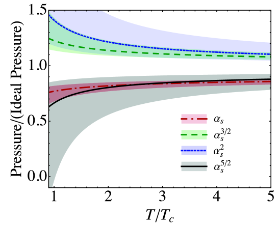
Figure 1: Weak-coupling expansion for the scaled pressure of pure-glue QCD. Shaded bands show the result of varying the renormalization scale $\mu$ by a factor of two around $\mu=2\pi T$.

The poor convergence of finite-temperature perturbative expansions of thermodynamic functions stems from the fact that at high temperature the classical solution is not described by massless gluons. Instead one must include plasma effects such as the screening of electric fields and Landau damping of excitations via a self-consistent hard-thermal-loop (HTL) resummation [15]. There are several ways of systematically reorganizing the perturbative expansion [16]. Here we will present the details of a new NNLO calculation which uses the hard-thermal-loop perturbation theory method [17, 18, 19, 22] and compare with previously obtained LO and NLO results.

The basic idea of the technique is to add and subtract an effective mass term from the bare Lagrangian and to associate the added piece with the free part of the Lagrangian and the subtracted piece with the interactions [23, 24]. However, in gauge theories, one cannot simply add and subtract a local mass term since this would violate gauge invariance [25, 26, 27]. Instead, one adds and subtracts an HTL improvement term which modifies the propagators and vertices self-consistently so that the reorganization is manifestly gauge invariant [25].

In this paper we discuss the calculation of thermodynamic functions of a gas of gluons at phenomenologically relevant temperatures using hard-thermal-loop perturbation theory. We present results at leading order (LO), next-to-leading order (NLO), and next-to-next-to-leading order (NNLO) and compare with available lattice data [28, 29] for the thermodynamic functions of SU(3) Yang-Mills theory. The calculation is based on a reorganization of the theory around hard-thermal-loop (HTL) quasiparticles. Our results indicate that the lattice data at temperatures $T\sim 2-3\;T_{c}$ are consistent with the quasiparticle picture. This is a non-trivial result since, in this temperature regime, the QCD coupling constant is neither infinitesimally weak nor infinitely strong with $g\sim 2$, or equivalently $\alpha_{s}=g^{2}/(4\pi)\sim 0.3$. Therefore, we have a crucial test of the quasiparticle picture in the intermediate coupling regime.

1 HTL perturbation theory

The Lagrangian density for pure-glue QCD in Minkowski space is

$${\cal L}_{\rm QCD} = -{1\over 2}{\rm Tr}\left[G_{\mu\nu}G^{\mu\nu}\right]+{\cal L}_{\rm gf}+{\cal L}_{\rm gh}+\Delta{\cal L}_{\rm QCD}\;,$$ (1)

where the field strength is $G^{\mu\nu}=\partial^{\mu}A^{\nu}-\partial^{\nu}A^{\mu}-ig[A^{\mu},A^{\nu}]$. The ghost term ${\cal L}_{\rm gh}$ depends on the gauge-fixing term ${\cal L}_{\rm gf}$. In this paper we choose the class of covariant gauges where the gauge-fixing term is

$${\cal L}_{\rm gf} = -{1\over\xi}{\rm Tr}\left[\left(\partial_{\mu}A^{\mu}\right)^{2}\right]\;.$$ (2)

The perturbative expansion in powers of $g$ generates ultraviolet divergences. The renormalizability of perturbative QCD guarantees that all divergences in physical quantities can be removed by renormalization of the coupling constant $\alpha_{s}=g^{2}/4\pi$. There is no need for wavefunction renormalization, because physical quantities are independent of the normalization of the field. There is also no need for renormalization of the gauge parameter, because physical quantities are independent of the gauge parameter.

Hard-thermal-loop perturbation theory (HTLpt) is a reorganization of the perturbation series for thermal QCD. The Lagrangian density is written as

$${\cal L}=\left({\cal L}_{\rm QCD}+{\cal L}_{\rm HTL}\right)\Big{|}_{g\to\sqrt{\delta}g}+\Delta{\cal L}_{\rm HTL}.$$ (3)

The HTL improvement term is

$${\cal L}_{\rm HTL}=-{1\over 2}(1-\delta)m_{D}^{2}{\rm Tr}\left(G_{\mu\alpha}\left\langle{y^{\alpha}y^{\beta}\over(y\cdot D)^{2}}\right\rangle_{\!\!y}G^{\mu}_{\;\;\beta}\right)\,,$$ (4)

where the covariant derivative is $D^{\mu}=\partial^{\mu}-igA^{\mu}$ and $y^{\mu}=(1,\hat{{\bf y}})$ is a light-like four-vector, and $\langle\ldots\rangle_{y}$ represents the average over the directions of $\hat{{\bf y}}$. The term (4) has the form of the effective Lagrangian that would be induced by a rotationally invariant ensemble of charged sources with infinitely high momentum. The parameter $m_{D}$ can be identified with the Debye screening mass. HTLpt is defined by treating $\delta$ as a formal expansion parameter.

The HTL perturbation expansion generates ultraviolet divergences. In perturbative QCD, renormalizability constrains the ultraviolet divergences to have a form that can be cancelled by the counterterm Lagrangian $\Delta{\cal L}_{\rm QCD}$. We will demonstrate that renormalized perturbation theory can be implemented by including a counterterm Lagrangian $\Delta{\cal L}_{\rm HTL}$ among the interaction terms in (3). There is no proof that the HTL perturbation expansion is renormalizable, so the general structure of the ultraviolet divergences is not known; however, it was shown in previous papers [17, 18] that it was possible to renormalize the NLO order HTLpt prediction for the free energy of QCD using only a vacuum counterterm, a Debye mass counterterm, and a fermion mass counterterm. In this paper we will show that this is also possible at NNLO. In particular, the only new counterterm we need to introduce is for the coupling constant $\alpha_{s}$, which coincides with its perturbative value giving rise to the standard one-loop running.

We find that the counterterms necessary to renormalize HTLpt at NNLO are

$$\delta\Delta\alpha_{s} = -{11N_{c}\over 12\pi\epsilon}\alpha_{s}^{2}\delta^{2}+{\cal O}(\delta^{3}\alpha^{3}_{s})\;,$$ (5)

$$\Delta m_{D}^{2} = \left(-{11N_{c}\over 12\pi\epsilon}\alpha_{s}\delta+{\cal O}(\delta^{2}\alpha_{s}^{2})\right)(1-\delta)m_{D}^{2}\;,$$ (6)

$$\Delta{\cal E}_{0} = \left({N_{c}^{2}-1\over 128\pi^{2}\epsilon}+{\cal O}(\delta\alpha_{s})\right)(1-\delta)^{2}m_{D}^{4}\;.$$ (7)

We note that the counterterm in Eq. (5) coincides with the perturbative one-loop running.

Physical observables are calculated in HTLpt by expanding them in powers of $\delta$, truncating at some specified order, and then setting $\delta=1$. This defines a reorganization of the perturbation series in which the effects of $m_{D}^{2}$ term in (4) are included to all orders but then systematically subtracted out at higher orders in perturbation theory by the $\delta m_{D}^{2}$ terms in (4). If we set $\delta=1$, the Lagrangian (3) reduces to the QCD Lagrangian (1).

If the expansion in $\delta$ could be calculated to all orders the final result would not depend on $m_{D}$ when we set $\delta=1$. However, any truncation of the expansion in $\delta$ produces results that depend on $m_{D}$. Some prescription is required to determine $m_{D}$ as a function of $T$ and $\alpha_{s}$. We will discuss several prescriptions in Sec. VI.

2 Diagrams for the thermodynamic potential

In this section, we list the expressions for the diagrams that contribute to the thermodynamic potential through order $\delta^{2}$ in HTL perturbation theory. The diagrams are shown in Figs. 2, and 3. A key to the diagrams is given in Fig. 4. The expressions here will be given in Euclidean space; however, in Appendix A we present the HTLpt Feynman rules in Minkowski space.

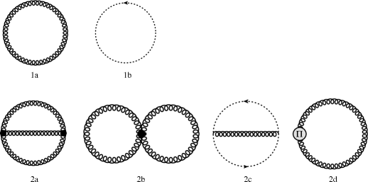
Figure 2: Diagrams contributing through NLO in HTLpt. The spiral lines are gluon propagators and the dotted lines are ghost propagators. A circle with a $\Pi$ indicates a gluon self-energy insertion. All propagators and vertices shown are HTL-resummed propagators and vertices.

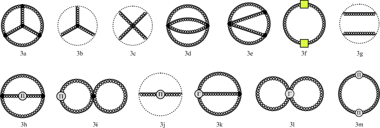
Figure 3: Diagrams contributing to NNLO in HTLpt which contribute through order $g^{5}$. The spiral lines are gluon propagators and the dotted lines are ghost propagators. A circle with a $\Pi$ indicates a gluon self-energy insertion The propagators are HTL-resummed propagators and the black dots indicate HTL-resummed vertices. The lettered vertices indicate that only the HTL correction is included. The yellow box denotes the insertion of the one-loop self-energy defined in Fig. 4.

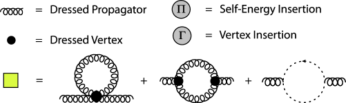
Figure 4: Key to the diagrams in Figs. 2 and 3.

The thermodynamic potential at leading order in HTL perturbation theory for QCD is

$$\Omega_{\rm LO}=(N_{c}^{2}-1){\cal F}_{\rm 1a+1b}+\Delta_{0}{\cal E}_{0}\;.$$ (8)

Here, ${\cal F}_{\rm 1a+1b}$ is the contribution from the gluon and ghost diagrams shown on the first line of Fig. 2

$$\!\!\!\!\!\!\!{\cal F}_{\rm 1a+1b}\!\! = \!\!-{1\over 2}\hbox{$\sum$}\!\!\!\!\!\!\!\int_{P}\!\left\{(d-1)\log\left[-\Delta_{T}(P)\right]+\log\Delta_{L}(P)\right\}.$$ (9)

The transverse and longitudinal HTL propagators $\Delta_{T}(P)$ and $\Delta_{L}(P)$ are given in (49) and (50). The leading-order vacuum counterterm $\Delta_{0}{\cal E}_{0}$ was determined in Ref. [17]:

$$\Delta_{0}{\cal E}_{0} = {N_{c}^{2}-1\over 128\pi^{2}\epsilon}m_{D}^{4}\;.$$ (10)

The thermodynamic potential at NLO in HTL perturbation theory can be written as

$$\Omega_{\rm NLO} = \Omega_{\rm LO}+(N_{c}^{2}-1)[{\cal F}_{\rm 2a}+{\cal F}_{\rm 2b}+{\cal F}_{\rm 2c}+{\cal F}_{\rm 2d}]$$ (11)

$$+\Delta_{1}{\cal E}_{0}+\Delta_{1}m_{D}^{2}{\partial\over\partial m_{D}^{2}}\Omega_{\rm LO}\;,$$

where $\Delta_{1}{\cal E}_{0}$ and $\Delta_{1}m_{D}^{2}$ are the terms of order $\delta$ in the vacuum energy density and mass counterterms:

$$\Delta_{1}{\cal E}_{0} = -{N_{c}^{2}-1\over 64\pi^{2}\epsilon}m_{D}^{4}\;,$$ (12)

$$\Delta_{1}m_{D}^{2} = -{11N_{c}\over 12\pi\epsilon}\alpha_{s}m_{D}^{2}\;.$$ (13)

The contributions from the two-loop diagrams with the three-gluon and four-gluon vertices are

$${\cal F}_{\rm 2a} = {N_{c}\over 12}g^{2}\hbox{$\sum$}\!\!\!\!\!\!\!\int_{PQ}\Gamma^{\mu\lambda\rho}(P,Q,R)\Gamma^{\nu\sigma\tau}(P,Q,R)\Delta^{\mu\nu}(P)$$ (14)

$$\times\Delta^{\lambda\sigma}(Q)\Delta^{\rho\tau}(R)\;,$$

$${\cal F}_{\rm 2b} = {N_{c}\over 8}g^{2}\hbox{$\sum$}\!\!\!\!\!\!\!\int_{PQ}\Gamma^{\mu\nu,\lambda\sigma}(P,-P,Q,-Q)\Delta^{\mu\nu}(P)$$ (15)

$$\times\Delta^{\lambda\sigma}(Q)\;,$$

where $R=Q-P$. For the corresponding diagrams, see the second line of Fig. 2.

The contribution from the ghost diagram is

$${\cal F}_{\rm 2c} = {N_{c}\over 2}g^{2}\hbox{$\sum$}\!\!\!\!\!\!\!\int_{PQ}{1\over Q^{2}}{1\over R^{2}}Q^{\mu}R^{\nu}\Delta^{\mu\nu}(P)\;.$$ (16)

The contribution from the HTL gluon counterterm diagram with a single gluon self-energy insertion is

$${\cal F}_{\rm 2d} = {1\over 2}\hbox{$\sum$}\!\!\!\!\!\!\!\int_{P}\Pi^{\mu\nu}(P)\Delta^{\mu\nu}(P)\;.$$ (17)

The thermodynamic potential at NNLO in HTL perturbation theory can be written as

$$\Omega_{\rm NNLO} = \Omega_{\rm NLO}+(N_{c}^{2}-1)\left[{\cal F}_{\rm 3a}+{\cal F}_{\rm 3b}+{\cal F}_{\rm 3c}+{\cal F}_{\rm 3d}+{\cal F}_{\rm 3e}+{\cal F}_{\rm 3f}+{\cal F}_{\rm 3g}+{\cal F}_{\rm 3h}+{\cal F}_{\rm 3i}+{\cal F}_{\rm 3j}+{\cal F}_{\rm 3k}\right.$$ (18)

$$\left.+{\cal F}_{\rm 3l}+{\cal F}_{\rm 3m}\right]+\Delta_{2}{\cal E}_{0}+\Delta_{2}m_{D}^{2}{\partial\over\partial m_{D}^{2}}\Omega_{\rm LO}+\Delta_{1}m_{D}^{2}{\partial\over\partial m_{D}^{2}}\Omega_{\rm NLO}$$

$$+{1\over 2}\left({\partial^{2}\over(\partial m_{D}^{2})^{2}}\Omega_{\rm LO}\right)\left(\Delta_{1}m_{D}^{2}\right)^{2}+(N_{c}^{2}-1){{\cal F}_{\rm 2a+2b+2c}\over\alpha_{s}}\Delta_{1}\alpha_{s}\;.$$

where $\Delta_{1}\alpha_{s}$, $\Delta_{2}m_{D}^{2}$, and $\Delta_{2}{\cal E}_{0}$ are the terms of order $\delta^{2}$ in the coupling constant, mass, and vacuum energy density counterterms:

$$\Delta_{1}\alpha_{s} = -{11N_{c}\over 12\pi\epsilon}\alpha_{s}^{2}\;,$$ (19)

$$\Delta_{2}m_{D}^{2} = {11N_{c}\over 12\pi\epsilon}\alpha_{s}m_{D}^{2}\;,$$ (20)

$$\Delta_{2}{\cal E}_{0} = {N_{c}^{2}-1\over 128\pi^{2}\epsilon}m_{D}^{4}\;.$$ (21)

The contributions from the three-loop diagrams are given by

$${\cal F}_{\rm 3a} = {N_{c}^{2}\over 24}g^{4}\hbox{$\sum$}\!\!\!\!\!\!\!\int_{PQR}\Gamma^{\alpha\beta\gamma}(P,Q,-P-Q)\Delta^{\alpha\theta}(P)\Delta^{\beta\mu}(Q)\Delta^{\gamma\sigma}(P+Q)\Gamma^{\mu\nu\delta}(-Q,-R,Q+R)\Delta^{\pi\nu}(R)$$ (22)

$$\times\Delta^{\delta\lambda}(Q+R)\Gamma^{\sigma{\lambda}\rho}(P+Q,-Q-R,R-P)\Delta^{\rho{\phi}}(R-P)\Gamma^{\theta\phi\pi}(-P,P-R,R)\;,$$

$${\cal F}_{\rm 3b} = {N_{c}^{2}\over 3}g^{4}\hbox{$\sum$}\!\!\!\!\!\!\!\int_{PQR}{{R}^{\alpha}(P+Q+R)^{\beta}(P+R)^{\gamma}\over R^{2}(P+R)^{2}(P+Q+R)^{2}}\Gamma^{\mu\lambda\nu}(-P,-Q,P+Q)\Delta^{\alpha\mu}(P)$$ (23)

$$\times\Delta^{\beta\nu}(P+Q)\Delta^{\gamma\lambda}(Q)\;,$$

$${\cal F}_{\rm 3c} = -{N_{c}^{2}\over 4}g^{4}\hbox{$\sum$}\!\!\!\!\!\!\!\int_{PQR}{(Q+R)^{\alpha}(R-P)^{\beta}(Q+R-P)^{\mu}R^{\nu}\over R^{2}(Q+R)^{2}(Q+R-P)^{2}(R-P)^{2}}\Delta^{\alpha\beta}(P)\Delta^{\mu\nu}(Q)\;,$$ (24)

$${\cal F}_{\rm 3d} = {N_{c}^{2}\over 48}\hbox{$\sum$}\!\!\!\!\!\!\!\int_{PQR}\Gamma^{\alpha\beta,\mu\nu}(P,Q,R,S)\Gamma^{\gamma\delta,\sigma\lambda}(P,Q,R,S)\Delta^{\alpha\gamma}(P)\Delta^{\beta\delta}(Q)\Delta^{\mu\sigma}(R)\Delta^{\nu\lambda}(S)\;,$$ (25)

$${\cal F}_{\rm 3e} = {-}{N_{c}^{2}\over{4}}\hbox{$\sum$}\!\!\!\!\!\!\!\int_{PQR}\Gamma^{\alpha\mu,\gamma\sigma}(P,Q,R,S)\Delta^{\alpha\beta}(P)\Delta^{\mu\nu}(Q)\Delta^{\gamma\delta}(R)\Delta^{\sigma\phi}(S)\Delta^{\theta\lambda}(P+Q)$$ (26)

$$\times\Gamma^{\beta\nu\theta}(-P,-Q,P+Q)\Gamma^{\lambda\delta\phi}({-P-Q,-R,-S)}\;,$$

$${\cal F}_{\rm 3f} = \hbox{$\sum$}\!\!\!\!\!\!\!\int_{P}\bar{\Pi}^{\mu\nu}(P)\Delta^{\nu\alpha}(P)\bar{\Pi}^{\alpha\beta}(P)\Delta^{\beta\mu}(P)\;,$$ (27)

$${\cal F}_{\rm 3g} = {-}{N_{c}^{2}\over 2}g^{4}\hbox{$\sum$}\!\!\!\!\!\!\!\int_{PQR}{P^{\alpha}(P+Q)^{\mu}P^{\nu}(P+R)^{\beta}\over P^{4}(P+Q)^{2}(P+R)^{2}}\Delta^{\mu\nu}(Q)\Delta^{\alpha\beta}(R)\;,$$ (28)

where $S=-(P+Q+R)$ and $\bar{\Pi}^{\mu\nu}(P)$ is the one-loop gluon self-energy defined by the yellow box in Fig. 4.

$$\bar{\Pi}^{\mu\nu}(P) = {1\over 2}N_{c}g^{2}\hbox{$\sum$}\!\!\!\!\!\!\!\int_{Q}\Gamma^{\mu\nu,\alpha\beta}(P,-P,Q,-Q)\Delta^{\alpha\beta}(Q)+{1\over 2}N_{c}g^{2}\hbox{$\sum$}\!\!\!\!\!\!\!\int_{Q}\Gamma^{\mu\alpha\beta}(P,Q,-P-Q)\Delta^{\alpha\gamma}(Q)$$ (29)

$$\times\Gamma^{\nu\gamma\delta}(P,Q,-P-Q)\Delta^{\beta}\delta(R)+N_{c}g^{2}\hbox{$\sum$}\!\!\!\!\!\!\!\int_{Q}{Q^{\mu}(P+Q)^{\nu}\over Q^{2}(P+Q)^{2}}\;.$$

The contributions from the two-loop diagrams with a single self-energy insertion are

$${\cal F}_{\rm 3h} = -{N_{c}\over 4}g^{2}\hbox{$\sum$}\!\!\!\!\!\!\!\int_{PQ}\Gamma^{\alpha\mu\nu}(P,Q,R)\Gamma^{\beta\gamma\delta}(P,Q,R)\Delta^{\alpha\sigma}(P)\Pi^{\sigma\lambda}(P)\Delta^{\lambda\beta}(P)\Delta^{\mu\gamma}(Q)\Delta^{\nu\delta}(R)\;,$$ (30)

$${\cal F}_{\rm 3i} = -{N_{c}\over 4}g^{2}\hbox{$\sum$}\!\!\!\!\!\!\!\int_{PQ}\Gamma^{\alpha\beta,\mu\nu}(P,-P,Q,-Q)\Delta^{\alpha\gamma}(P)\Pi^{\gamma\delta}(P)\Delta^{\delta\beta}(P)\Delta^{\mu\nu}(Q)\;,$$ (31)

$${\cal F}_{\rm 3j} = -{N_{c}\over 2}g^{2}\hbox{$\sum$}\!\!\!\!\!\!\!\int_{PQ}{P^{\alpha}(P+Q)^{\beta}\over P^{2}(P+Q)^{2}}\Delta^{\alpha\mu}(Q)\Pi^{\mu\nu}(Q)\Delta^{\nu\beta}(Q)\;,$$ (32)

where $R=Q-P$.

The two-loop diagrams with a subtracted vertex is

$${\cal F}_{\rm 3k} = {N_{c}\over 6}g^{2}m_{D}^{2}\hbox{$\sum$}\!\!\!\!\!\!\!\int_{PQ}{\cal T}^{\mu\lambda\rho}(P,Q,R)\Gamma^{\nu\sigma\tau}(P,Q,R)\Delta^{\mu\nu}(P)$$ (33)

$$\times\Delta^{\lambda\sigma}(Q)\Delta^{\rho\tau}(R)\;,$$

$${\cal F}_{\rm 3l} = {N_{c}\over 8}g^{2}m_{D}^{2}\hbox{$\sum$}\!\!\!\!\!\!\!\int_{PQ}{\cal T}^{\mu\nu,\lambda\sigma}(P,-P,Q,-Q)\Delta^{\mu\nu}(P)$$ (34)

$$\times\Delta^{\lambda\sigma}(Q)\;,$$

where $R=Q-P$.

The contribution from the HTL gluon counterterm diagram with two gluon self-energy insertions is

$${\cal F}_{\rm 3m} = -{1\over 4}\hbox{$\sum$}\!\!\!\!\!\!\!\int_{P}\Pi^{\mu\nu}(P)\Delta^{\nu\alpha}(P)\Pi^{\alpha\beta}(P)\Delta^{\beta\mu}(P)\;.$$ (35)

3 Expansion in $m_{D}/T$

In the papers [17, 18, 19, 20, 21], the free energy was reduced to scalar sum-integrals. It was clear that evaluating these scalar sum-integrals exactly was intractable and the sum-integrals were calculated approximately by expanding them in powers of $m_{D}/T$. We will follow the same strategy in this paper and carry out the expansion to high enough order to include all terms through order $g^{5}$ if $m_{D}$ is taken to be of order $g$.

The free energy can be divided into contributions from hard and soft momenta. In the one-loop diagrams, the contributions are either hard $(h)$ or soft $(s)$, while at the two-loop level, there are hard-hard $(hh)$, hard-soft $(hs)$, and soft-soft $(ss)$ contributions. At three loops there are hard-hard-hard $(hhh)$, hard-hard-soft $(hhs)$, hard-soft-soft $(hss)$, and soft-soft-soft $(sss)$ contributions.

3.1 Leading order

3.1.1 Hard contribution

For hard momenta, the self-energies are suppressed by $m_{D}/T$ relative to the propagators, so we can expand in powers of $\Pi_{T}(P)$ and $\Pi_{L}(P)$.

For the one-loop graphs $\rm(1a)$ and $\rm(1b)$, we need to expand to second order in $m^{2}_{D}$:

$${\cal F}_{\rm 1a+1b}^{(h)} = {1\over 2}(d-1)\hbox{$\sum$}\!\!\!\!\!\!\!\int_{P}\log\left(P^{2}\right)+{1\over 2}m_{D}^{2}\hbox{$\sum$}\!\!\!\!\!\!\!\int_{P}{1\over P^{2}}$$ (36)

$$-{1\over 4(d-1)}m_{D}^{4}\hbox{$\sum$}\!\!\!\!\!\!\!\int_{P}\left[{1\over P^{4}}-2{1\over p^{2}P^{2}}-2d{1\over p^{4}}{\cal T}_{P}+2{1\over p^{2}P^{2}}{\cal T}_{P}+d{1\over p^{4}}\left({\cal T}_{P}\right)^{2}\right]$$

$$= -{\pi^{2}\over 45}T^{4}+{1\over 24}\left[1+\left(2+2{\zeta^{\prime}(-1)\over\zeta(-1)}\right)\epsilon\right]\left({\mu\over 4\pi T}\right)^{2\epsilon}m_{D}^{2}T^{2}$$

$$-{1\over 128\pi^{2}}\left({1\over\epsilon}-7+2\gamma_{E}+{2\pi^{2}\over 3}\right)\left({\mu\over 4\pi T}\right)^{2\epsilon}m_{D}^{4}\;.$$

3.1.2 Soft contribution

The soft contribution in the diagrams $(1a+1b)$ arises from the $P_{0}=0$ term in the sum-integral. At soft momentum $P=(0,{\bf p})$, the HTL self-energy functions reduce to $\Pi_{T}(P)=0$ and $\Pi_{L}(P)=m_{D}^{2}$. The transverse term vanishes in dimensional regularization because there is no momentum scale in the integral over ${\bf p}$. Thus the soft contributions come from the longitudinal term only and read

$${\cal F}^{(s)}_{\rm 1a+1b} = {1\over 2}T\int_{p}\log\left(p^{2}+m_{D}^{2}\right)$$ (37)

$$= -{m_{D}^{3}T\over 12\pi}\left({\mu\over 2m}\right)^{2\epsilon}\left[1+{8\over 3}\epsilon\right]\;.$$

We have kept the order-$\epsilon$ in the $m_{D}^{2}$ and $m_{D}^{3}$ terms, respectively in Eqs. (36) and (37) since they contribute in the counterterms at next-to-leading order.

3.2 Next-to-leading order

3.2.1 Hard contribution

The one-loop graph with a gluon self-energy insertion $\rm(2d)$ has an explicit factor of $m_{D}^{2}$ and so we need only to expand the sum-integal to first order in $m_{D}^{2}$:

$${\cal F}_{\rm 2d}^{(h)}\!\! = \!\!-{1\over 2}m_{D}^{2}\hbox{$\sum$}\!\!\!\!\!\!\!\int_{P}{1\over P^{2}}+{1\over 2(d-1)}m_{D}^{4}\hbox{$\sum$}\!\!\!\!\!\!\!\int_{P}\left[{1\over P^{4}}-2{1\over p^{2}P^{2}}-2d{1\over p^{4}}{\cal T}_{P}+2{1\over p^{2}P^{2}}{\cal T}_{P}+d{1\over p^{4}}\left({\cal T}_{P}\right)^{2}\right]$$ (38)

$$= \!\!-{1\over 24}\left[1+\left(2+2{\zeta^{\prime}(-1)\over\zeta(-1)}\right)\epsilon\right]\left({\mu\over 4\pi T}\right)^{2\epsilon}m_{D}^{2}T^{2}+{1\over 64\pi^{2}}\left({1\over\epsilon}-7+2\gamma_{E}+{2\pi^{2}\over 3}\right)\left({\mu\over 4\pi T}\right)^{2\epsilon}m_{D}^{4}\;.$$

3.2.2 Soft contribution

The soft contribution from $\rm(2d)$ arises from the $P_{0}=0$ term in the sum-integral. Only the longitudinal part $\Pi_{L}(P)$ of the self-energy contributes and reads

$${\cal F}^{(s)}_{\rm 2d} = -{1\over 2}m_{D}^{2}T\int_{p}{1\over p^{2}+m_{D}^{2}}$$ (39)

$$= {m^{3}_{D}T\over 8\pi}\left({\mu\over 2m_{D}}\right)^{2\epsilon}\left[1+2\epsilon\right]\;.$$

3.2.3 $(hh)$ contributions

For hard momenta, the self-energies are suppressed by $m_{D}/T$ relative to the propagators, so we can expand in powers of $\Pi_{T}$ and $\Pi_{L}$. The two-loop contribution was calculated in Ref. [18] and reads

$${\cal F}^{(hh)}_{\rm 2a+2b+2c} = {N_{c}\over 4}g^{2}(d-1)^{2}\hbox{$\sum$}\!\!\!\!\!\!\!\int_{PQ}\left[{1\over P^{2}}{1\over Q^{2}}\right]+{N_{c}\over 4}g^{2}m_{D}^{2}\hbox{$\sum$}\!\!\!\!\!\!\!\int_{PQ}\left[-2(d-1){1\over P^{2}}{1\over Q^{4}}+2(d-2){1\over P^{2}}{1\over q^{2}Q^{2}}\right.$$ (40)

$$\left.+(d+2){1\over Q^{2}R^{2}r^{2}}-2d{P\cdot Q\over P^{2}Q^{2}r^{4}}-4d{q^{2}\over P^{2}Q^{2}r^{4}}+4{q^{2}\over P^{2}Q^{2}r^{2}R^{2}}-2(d-1){1\over P^{2}}{1\over q^{2}Q^{2}}{\cal T}_{Q}\right.$$

$$-(d+1){1\over P^{2}Q^{2}r^{2}}{\cal T}_{R}\left.+4d{q^{2}\over P^{2}Q^{2}r^{4}}{\cal T}_{R}+2d{P\cdot Q\over P^{2}Q^{2}r^{4}}{\cal T}_{R}\right]\;.$$

Using the expressions for the sum-integrals listed in Appendix B, we obtain

$${\cal F}^{(hh)}_{\rm 2a+2b+2c} = {\pi^{2}\over 12}{N_{c}\alpha_{s}\over 3\pi}\left[1+\left(2+4{\zeta^{\prime}(-1)\over\zeta(-1)}\right)\epsilon\right]\left({\mu\over 4\pi T}\right)^{4\epsilon}T^{4}$$ (41)

$$-{7\over 96}\left[{1\over\epsilon}+4.621\right]{N_{c}\alpha_{s}\over 3\pi}\left({\mu\over 4\pi T}\right)^{4\epsilon}m^{2}_{D}T^{2}\;.$$

3.2.4 $(hs)$ contributions

In the $(hs)$ region, the momentum $P$ is soft. The momenta $Q$ and $R$ are always hard. The function that multiplies the soft propagator $\Delta_{T}(0,{\bf p})$, $\Delta_{L}(0,{\bf p})$ or $\Delta_{X}(0,{\bf p})$ can be expanded in powers of the soft momentum ${\bf p}$. In the case of $\Delta_{T}(0,{\bf p})$, the resulting integrals over ${\bf p}$ have no scale and they vanish in dimensional regularization. The integration measure $\int_{p}$ scales like $m_{D}^{3}$, the soft propagators $\Delta_{L}(0,{\bf p})$ and $\Delta_{X}(0,{\bf p})$ scale like $1/m_{D}^{2}$, and every power of $p$ in the numerator scales like $m_{D}$. The two-loop contribution was calculated in Ref. [18] and reads

$${\cal F}_{\rm 2a+2b+2c}^{(hs)} = {N_{c}\over 2}g^{2}T\int_{p}{1\over p^{2}+m_{D}^{2}}\hbox{$\sum$}\!\!\!\!\!\!\!\int_{Q}\left[-(d-1){1\over Q^{2}}+2(d-1){q^{2}\over Q^{4}}\right]+N_{c}g^{2}m_{D}^{2}T\int_{p}{1\over p^{2}+m_{D}^{2}}$$ (42)

$$\hbox{$\sum$}\!\!\!\!\!\!\!\int_{Q}\left[-(d-4){1\over Q^{4}}+{(d-1)(d+2)\over d}{q^{2}\over Q^{6}}-{4(d-1)\over d}{q^{4}\over Q^{8}}\right]\;.$$

In order to facilitate the calculations, it proves useful to isolate the terms that are specific to HTL perturbation theory. After integrating by parts and using the results from Zhai and Kastening [11], we can write

$${\cal F}_{\rm 2a+2b+2c}^{(hs)} = {N_{c}\over 2}g^{2}T(d-1)^{2}\int_{p}{1\over p^{2}+m_{D}^{2}}\hbox{$\sum$}\!\!\!\!\!\!\!\int_{Q}{1\over Q^{2}}+{N_{c}\over 12}[d^{2}-5d+16]g^{2}Tm_{D}^{2}\int_{p}{1\over p^{2}+m_{D}^{2}}\hbox{$\sum$}\!\!\!\!\!\!\!\int_{Q}{1\over Q^{4}}$$ (43)

$$-{N_{c}\over 2}(d-5)g^{2}Tm_{D}^{2}\int_{p}{1\over p^{2}+m_{D}^{2}}\hbox{$\sum$}\!\!\!\!\!\!\!\int_{Q}{1\over Q^{4}}\;.$$

Using the expressions for the integrals and sum-integrals in Appendices B and C, we obtain

$${\cal F}^{(hs)}_{\rm 2a+2b+2c} = -{\pi\over 2}{N_{c}\alpha_{s}\over 3\pi}m_{D}T^{3}\left[1+\left(2+2{\zeta^{\prime}(-1)\over\zeta(-1)}\right)\epsilon\right]\left({\mu\over 4\pi T}\right)^{2\epsilon}\left({\mu\over 2m_{D}}\right)^{2\epsilon}$$ (44)

$$-{11\over 32\pi}\left({1\over\epsilon}+{27\over 11}+2\gamma_{E}\right){N_{c}\alpha_{s}\over 3\pi}\left({\mu\over 4\pi T}\right)^{2\epsilon}\left({\mu\over 2m_{D}}\right)^{2\epsilon}m_{D}^{3}T\;.$$

3.2.5 $(ss)$ contribution

The $(ss)$ contribution to the free energy is given by a two-loop calculation in electrostatic QCD (EQCD) in three dimensions. This calculation was carried out in Ref. [9] by Braaten and Nieto. Alternatively, one can isolate the $(ss)$ contributions from the two-loop diagrams which were calculated by Arnold and Zhai in Ref. [6]. In Ref. [18], this contribution was calculated and agrees with earlier results. One finds

$${\cal F}^{(ss)}_{\rm 2a+2b+2c} = {1\over 4}N_{c}g^{2}T^{2}\int_{pq}{p^{2}+4m_{D}^{2}\over p^{2}(q^{2}+m_{D}^{2})(r^{2}+m_{D}^{2})}$$ (45)

$$= {3\over 16}\left[{1\over\epsilon}+3\right]{N_{c}\alpha_{s}\over 3\pi}\left({\mu\over 2m_{D}}\right)^{4\epsilon}m_{D}^{2}T^{2}\;.$$

We have kept the order $\epsilon$ in terms Eqs. (38), (39), (41), and (44) since they contribute in the counterterms at NNLO.

3.3 Next-to-next-to-leading order

3.3.1 Hard contribution

The one-loop graph with two gluon self-energy insertions $\rm(3m)$ is proportional to $m_{D}^{4}$ and so must be expanded to zeroth order in $m_{D}^{2}$

$${\cal F}_{\rm 3m}^{(h)} = -{1\over 4(d-1)}m_{D}^{4}\hbox{$\sum$}\!\!\!\!\!\!\!\int_{P}\left[{1\over P^{4}}-2{1\over p^{2}P^{2}}-2d{1\over p^{4}}{\cal T}_{P}+2{1\over p^{2}P^{2}}{\cal T}_{P}+d{1\over p^{4}}\left({\cal T}_{P}\right)^{2}\right]$$ (46)

$$= -{1\over 128\pi^{2}}\left({1\over\epsilon}-7+2\gamma_{E}+{2\pi^{2}\over 3}\right)\left({\mu\over 4\pi T}\right)^{2\epsilon}m_{D}^{4}\,.$$

3.3.2 Soft contribution

The soft contribution from $\rm(3m)$ arises from the $P_{0}=0$ term in the sum-integral. Only the longitudinal part $\Pi_{L}(P)$ of the self-energy contributes and reads

$${\cal F}^{(s)}_{\rm 3m} = -{1\over 4}m_{D}^{4}T\int_{p}{1\over(p^{2}+m_{D}^{2})^{2}}$$ (47)

$$= -{m^{3}_{D}T\over 32\pi}\;.$$

3.3.3 $(hh)$ contributions

We also need the $(hh)$ contribution from the diagrams $\rm(3h)-(3l)$. We calculate their contributions by expanding the two-loop diagrams $\rm(2a)-(2c)$ to first order in $m_{D}^{2}$. This yields

$${\cal F}^{(hh)}_{\rm 3h-3l} = -{N_{c}\over 4}g^{2}m_{D}^{2}\hbox{$\sum$}\!\!\!\!\!\!\!\int_{PQ}\left[-2(d-1){1\over P^{2}}{1\over Q^{4}}+2(d-2){1\over P^{2}}{1\over q^{2}Q^{2}}+(d+2){1\over Q^{2}R^{2}r^{2}}\right.$$ (48)

$$\left.-2d{P\cdot Q\over P^{2}Q^{2}r^{4}}-4d{q^{2}\over P^{2}Q^{2}r^{4}}+4{q^{2}\over P^{2}Q^{2}r^{2}R^{2}}-2(d-1){1\over P^{2}}{1\over q^{2}Q^{2}}{\cal T}_{Q}\right.$$

$$\left.-(d+1){1\over P^{2}Q^{2}r^{2}}{\cal T}_{R}+4d{q^{2}\over P^{2}Q^{2}r^{4}}{\cal T}_{R}+2d{P\cdot Q\over P^{2}Q^{2}r^{4}}{\cal T}_{R}\right]$$

$$= {7\over 96}\left[{1\over\epsilon}+4.621\right]{N_{c}\alpha_{s}\over 3\pi}\left({\mu\over 4\pi T}\right)^{4\epsilon}m^{2}_{D}T^{2}\;.$$

3.3.4 $(hs)$ contributions

We also need the $(hs)$ contribution from the diagrams $\rm(3h)-(3l)$. Again we calculate their contributions by expanding the two-loop diagrams $\rm(2a)-(2c)$ to first order in $m_{D}^{2}$. This yields

$${\cal F}_{\rm 3h-3l}^{(hs)} = {N_{c}\over 2}g^{2}(d-1)^{2}m_{D}^{2}T\int_{p}{1\over(p^{2}+m_{D}^{2})^{2}}\hbox{$\sum$}\!\!\!\!\!\!\!\int_{Q}{1\over Q^{2}}$$ (49)

$$\hskip 14.22636pt-{N_{c}\over 12}g^{2}m_{D}^{2}T\left[d^{2}-5d+16\right]\int_{p}{p^{2}\over(p^{2}+m_{D}^{2})^{2}}\hbox{$\sum$}\!\!\!\!\!\!\!\int_{Q}{1\over Q^{4}}$$

$$\hskip 28.45274pt+{N_{c}\over 2}g^{2}(d-5)m_{D}^{2}T\int_{p}{p^{2}\over(p^{2}+m_{D}^{2})^{2}}\hbox{$\sum$}\!\!\!\!\!\!\!\int_{Q}{1\over Q^{4}}\;.$$

This yields

$${\cal F}_{\rm 3h-3l}^{(hs)} = {\pi\over 4}{N_{c}\alpha_{s}\over 3\pi}m_{D}T^{3}+{33\over 64\pi}\left({1\over\epsilon}+{59\over 33}+2\gamma_{E}\right){N_{c}\alpha_{s}\over 3\pi}\left({\mu\over 4\pi T}\right)^{2\epsilon}\left({\mu\over 2m_{D}}\right)^{2\epsilon}m_{D}^{3}T\;.$$

3.3.5 $(ss)$ contribution

The $(ss)$ contribution from the two-loop diagrams with a single self-energy insertion or vertex correction can be obtained by expanding the two-loop result in powers of $m_{D}^{2}$. This yields

$${\cal F}^{(ss)}_{\rm 3h-3l} = -{1\over 4}N_{c}g^{2}m_{D}^{2}T^{2}\int_{pq}\left[{4\over p^{2}(q^{2}+m^{2}_{D})(r^{2}+m_{D}^{2})}-{2(p^{2}+4m_{D}^{2})\over p^{2}(q^{2}+m^{2}_{D})^{2}(r^{2}+m_{D}^{2})}\right]$$ (51)

$$= -{3\over 16}\left[{1\over\epsilon}+1\right]{N_{c}\alpha_{s}\over 3\pi}\left({\mu\over 2m_{D}}\right)^{4\epsilon}m_{D}^{2}T^{2}\;.$$

We have verified this by explicitly calculating the relevant diagrams.

3.3.6 $(hhh)$ contribution

If all the three loop momenta are hard, we can obtain the $m_{D}/T$ expansion simply by expanding in powers of $m_{D}^{2}$. To obtain the expansion through order $g^{5}$, we can use bare propagators and vertices. The contributions from the three-loop diagrams were first calculated by Arnold and Zhai in Ref. [6], and later by Braaten and Nieto [9]. One finds

$${\cal F}^{(hhh)}_{\rm 3a-3g} = {N_{c}^{2}\over 4}g^{4}(d-1)^{2}\hbox{$\sum$}\!\!\!\!\!\!\!\int_{PQR}\Biggl{[}-(d-5){1\over P^{2}Q^{2}R^{4}}-{1\over 2}{1\over P^{2}Q^{2}R^{2}(P+Q+R)^{2}}$$

$$\hskip 133.72795pt-{(P-Q)^{4}\over P^{2}Q^{2}R^{4}(Q-R)^{2}(R-P)^{2}}\Biggr{]}$$

$$= -{25\pi^{2}\over 48}\left({N_{c}\alpha_{s}\over 3\pi}\right)^{2}\left[{1\over\epsilon}+{238\over 125}+{12\over 25}\gamma_{E}+{176\over 25}{\zeta^{\prime}(-1)\over\zeta(-1)}-{38\over 25}{\zeta^{\prime}(-3)\over\zeta(-3)}\right]\left({\mu\over 4\pi T}\right)^{6\epsilon}T^{4}\,.$$

3.3.7 $(hhs)$ contributions

All the diagrams except $\rm(3f)$ are infrared finite in the limit $m_{D}\rightarrow 0$. This implies that the $g^{5}$ contribution is given by using a dressed longitudinal propagator and bare vertices. The ring diagram $\rm(3f)$ is infrared divergent in that limit. The contribution through $g^{5}$ is obtained by expanding in powers of self-energies and vertices and one obtains

$${\cal F}^{(hhs)}_{\rm 3a-3g} = -{N_{c}^{2}\over 4}g^{4}T(d-1)^{4}\int_{p}{1\over(p^{2}+m_{D}^{2})^{2}}\hbox{$\sum$}\!\!\!\!\!\!\!\int_{QR}{1\over Q^{2}R^{2}}$$ (53)

$$+{N_{c}^{2}\over 12}g^{4}T(d-1)^{2}\left[d^{2}-11d+46\right]\int_{p}{p^{2}\over(p^{2}+m_{D}^{2})^{2}}\hbox{$\sum$}\!\!\!\!\!\!\!\int_{QR}{1\over Q^{2}R^{4}}$$

$$= -{\pi^{3}\over 2}\left({N_{c}\alpha_{s}\over 3\pi}\right)^{2}{T^{5}\over m_{D}}$$

$$-{33\pi\over 16}\left({N_{c}\alpha_{s}\over 3\pi}\right)^{2}\left[{1\over\epsilon}+{59\over 33}+2\gamma_{E}+2{\zeta^{\prime}(-1)\over\zeta(-1)}\right]m_{D}T^{3}\left({\mu\over 2m_{D}}\right)^{2\epsilon}\left({\mu\over 4\pi T}\right)^{4\epsilon}\;.$$

3.3.8 $(hss)$ contribution

For all the diagrams that are infrared safe, the $(hss)$ contribution is of order $g^{4}m_{D}^{2}$, i.e. $g^{6}$ and can be ignored. The infrared divergent diagrams contribute as follows

$${\cal F}^{(hss)}_{\rm 3a-3g} = {1\over 4}g^{4}T^{2}N_{c}^{2}(d-1)^{2}\int_{pq}\left[{4\over p^{2}(q^{2}+m^{2}_{D})(r^{2}+m_{D}^{2})}-{2(p^{2}+4m_{D}^{2})\over p^{2}(q^{2}+m^{2}_{D})^{2}(r^{2}+m_{D}^{2})}\right]\hbox{$\sum$}\!\!\!\!\!\!\!\int_{R}{1\over R^{2}}$$ (54)

$$= {3\pi^{2}\over 4}\left[{1\over\epsilon}+1+2{\zeta^{\prime}(-1)\over\zeta(-1)}\right]\left({N_{c}\alpha_{s}\over 3\pi}\right)^{2}\left({\mu\over 2m_{D}}\right)^{4\epsilon}\left({\mu\over 4\pi T}\right)^{2\epsilon}T^{4}\;.$$

3.3.9 $(sss)$ contribution

The $(sss)$ contribution to the free energy is given by a three-loop calculation of the free energy of Electrostatic QCD in three dimensions. This calculation was performed in Ref. [9]. Alternatively, one can isolate the $(sss)$ contributions from the diagrams listed in Ref. [6]. The result is

$${\cal F}^{(sss)}_{\rm 3a-3g} = N_{c}^{2}g^{4}T^{3}\int_{pqr}\left\{-{1\over 4}{1\over(p^{2}+m^{2}_{D})(q^{2}+m^{2}_{D})(r^{2}+m^{2}_{D})^{2}}\right.$$ (55)

$$\left.+{2\over(p^{2}+m^{2}_{D})(q^{2}+m^{2}_{D})(r^{2}+m^{2}_{D})({\bf q}-{\bf r})^{2}}\right.$$

$$\left.-{2m_{D}^{2}\over(p^{2}+m^{2}_{D})(q^{2}+m^{2}_{D})(r^{2}+m^{2}_{D})^{2}({\bf q}-{\bf r})^{2}}\right.$$

$$\left.-{m_{D}^{2}\over(p^{2}+m^{2}_{D})(q^{2}+m^{2}_{D})(r^{2}+m^{2}_{D})({\bf q}-{\bf r})^{4}}\right.$$

$$\left.-{1\over 4}{({\bf p}-{\bf q})^{2}\over(p^{2}+m^{2}_{D})(q^{2}+m^{2}_{D})(r^{2}+m^{2}_{D})({\bf q}-{\bf r})^{2}({\bf r}-{\bf p})^{2}}\right.$$

$$\left.-{1\over 2}(d-2){1\over(p^{2}+m^{2}_{D})(q^{2}+m^{2}_{D})({\bf q}-{\bf r})^{2}({\bf r}-{\bf p})^{2}}\right.$$

$$\left.+{1\over 2}(3-d){(r^{2}+m^{2}_{D})\over(p^{2}+m^{2}_{D})(q^{2}+m^{2}_{D})({\bf p}-{\bf q})^{2}({\bf q}-{\bf r})^{2}({\bf r}-{\bf p})^{2}}\right.$$

$$\left.-{1\over 2}(d-2){(r^{2}+m^{2}_{D})^{2}\over(p^{2}+m^{2}_{D})(q^{2}+m^{2}_{D})({\bf p}-{\bf q})^{4}({\bf q}-{\bf r})^{2}({\bf r}-{\bf p})^{2}}\right.$$

$$\left.+{4m_{D}^{2}\over(p^{2}+m^{2}_{D})(q^{2}+m^{2}_{D})(r^{2}+m^{2}_{D})({\bf q}-{\bf r})^{2}({\bf r}-{\bf p})^{2}}\right.$$

$$\left.+{2m_{D}^{2}\over(p^{2}+m^{2}_{D})(q^{2}+m^{2}_{D})({\bf p}-{\bf q})^{2}({\bf q}-{\bf r})^{2}({\bf r}-{\bf p})^{2}}\right.$$

$$\left.-{4m_{D}^{4}\over(p^{2}+m^{2}_{D})(q^{2}+m^{2}_{D})(r^{2}+m^{2}_{D})^{2}({\bf q}-{\bf r})^{2}({\bf r}-{\bf p})^{2}}\right.$$

$$\left.-{3\over 8}{1\over(p^{2}+m^{2}_{D})(q^{2}+m^{2}_{D})[({\bf q}-{\bf r})^{2}+m^{2}_{D}][({\bf r}-{\bf p})^{2}+m^{2}_{D})]}\right.$$

$$\left.-{1\over 2}{({\bf p}-{\bf q})^{2}\over(p^{2}+m^{2}_{D})(q^{2}+m^{2}_{D})[({\bf q}-{\bf r})^{2}+m^{2}_{D}][({\bf r}-{\bf p})^{2}+m^{2}_{D}]r^{2}}\right.$$

$$\left.-{1\over 4}{({\bf p}-{\bf q})^{4}\over(p^{2}+m^{2}_{D})(q^{2}+m^{2}_{D})[({\bf q}-{\bf r})^{2}+m^{2}_{D}][({\bf r}-{\bf p})^{2}+m^{2}_{D}]r^{4}}\right.$$

$$\left.-{2m_{D}^{2}\over(p^{2}+m^{2}_{D})(q^{2}+m^{2}_{D})[({\bf q}-{\bf r})^{2}+m^{2}_{D}][({\bf r}-{\bf p})^{2}+m^{2}_{D})]r^{2}}\right.$$

$$\left.-m_{D}^{2}{({\bf p}-{\bf q})^{2}\over(p^{2}+m^{2}_{D})(q^{2}+m^{2}_{D})[({\bf q}-{\bf r})^{2}+m^{2}_{D}][({\bf r}-{\bf p})^{2}+m^{2}_{D}]r^{4}}\right.$$

$$\left.-m_{D}^{4}{1\over(p^{2}+m^{2}_{D})(q^{2}+m^{2}_{D})[({\bf q}-{\bf r})^{2}+m^{2}_{D}][({\bf r}-{\bf p})^{2}+m^{2}_{D}]r^{2}({\bf p}-{\bf q})^{2}}\right.$$

$$\left.-{m_{D}^{4}\over(p^{2}+m^{2}_{D})(q^{2}+m^{2}_{D})[({\bf q}-{\bf r})^{2}+m^{2}_{D}][({\bf r}-{\bf p})^{2}+m^{2}_{D}]r^{4}}\right.$$

$$\left.-{1\over 4}{(q^{2}+m^{2}_{D})\over(p^{2}+m^{2}_{D})[({\bf r}-{\bf p})^{2}+m^{2}_{D}][({\bf q}-{\bf r})^{2}+m^{2}_{D}]r^{2}({\bf p}-{\bf q})^{2}}\right\}\;.$$

The expression for the integrals are given in Appendix C. Adding Eqs. (31)– (43), the final result is

$${\cal F}^{(sss)}_{\rm 3a-3g} = {9\pi\over 4}\left({N_{c}\alpha_{s}\over 3\pi}\right)^{2}\left[{89\over 24}-{11\over 6}\log 2+{1\over 6}\pi^{2}\right]m_{D}T^{3}\;.$$ (56)

Note that all the poles in $\epsilon$ cancel.

4 The thermodynamic potential

In this section we present the final renormalized thermodynamic potential explicitly through order $\delta^{2}$, aka NNLO. The final NNLO expression is completely analytic; however, there are some numerically determined constants which remain in the final expressions at NLO.

4.1 Leading order

The leading order thermodynamic potential is given by the contribution from the diagrams $\rm(1a)$ and $\rm(1b)$.

$$\Omega_{\rm 1-loop} = {\cal F}_{\rm ideal}\left\{1-{15\over 2}\hat{m}_{D}^{2}+30\hat{m}_{D}^{3}+{45\over 8}\left({1\over\epsilon}+2\log{\hat{\mu}\over 2}-7+2\gamma_{E}+{2\pi^{2}\over 3}\right)\hat{m}_{D}^{4}\right\},$$

where ${\cal F}_{\rm ideal}$ is the free energy of a gas of $N_{c}^{2}-1$ massless spin-one bosons and $\hat{m}_{D}$ and $\hat{\mu}$ are dimensionless variables:

$${\cal F}_{\rm ideal} = \left(N_{c}^{2}-1\right)\left(-{\pi^{2}\over 45}T^{4}\right)\;,$$ (58)

$$\hat{m}_{D} = {m_{D}\over 2\pi T}\;,$$ (59)

$$\hat{\mu} = {\mu\over 2\pi T}\;.$$ (60)

The complete expression for the leading order thermodynamic potential is given by adding the leading vacuum energy counterterm (10) to Eq. (LABEL:Omega-1):

$$\Omega_{\rm LO} = {\cal F}_{\rm ideal}\left\{1-{15\over 2}\hat{m}_{D}^{2}+30\hat{m}_{D}^{3}+{45\over 4}\left(\log{\hat{\mu}\over 2}-{7\over 2}+\gamma_{E}+{\pi^{2}\over 3}\right)\hat{m}_{D}^{4}\right\}\;.$$ (61)

4.2 Next-to-leading order

The renormalization contributions at first order in $\delta$ are

$$\Delta\Omega_{1} = \Delta_{1}{\cal E}+\Delta_{1}m_{D}^{2}{\partial\over\partial m_{D}^{2}}\Omega_{\rm LO}$$ (62)

Using the results listed in Eqs. (12) and (13) the complete contribution from the counterterm at first order in $\delta$ is

$$\Delta\Omega_{1} = {\cal F}_{\rm ideal}\Bigg{\{}{45\over 4\epsilon}\hat{m}_{D}^{4}+{165\over 8}\Bigg{[}{1\over\epsilon}+2\log{\hat{\mu}\over 2}+2{\zeta^{\prime}(-1)\over\zeta(-1)}+2\bigg{]}{N_{c}\alpha_{s}\over 3\pi}\hat{m}_{D}^{2}$$ (63)

$$-{495\over 4}\left[{1\over\epsilon}+2\log{\hat{\mu}\over 2}-2\log\hat{m}_{D}+2\right]{N_{c}\alpha_{s}\over 3\pi}\hat{m}_{D}^{3}\bigg{\}}\;.$$

The NLO thermodynamic potential reads

$$\Omega_{\rm NLO} = {\cal F}_{\rm ideal}\Bigg{\{}1-15\hat{m}_{D}^{3}-{45\over 4}\left(\log\hat{\mu\over 2}-{7\over 2}+\gamma_{E}+{\pi^{2}\over 3}\right)\hat{m}_{D}^{4}+\Bigg{[}-{15\over 4}+45\hat{m}_{D}$$

$$-{165\over 4}\left(\log{\hat{\mu}\over 2}-{36\over 11}\log\hat{m}_{D}-2.001\right)\hat{m}_{D}^{2}+{495\over 2}\left(\log{\hat{\mu}\over 2}+{5\over 22}+\gamma_{E}\right)\!\!\hat{m}_{D}^{3}\Bigg{]}{N_{c}\alpha_{s}\over 3\pi}\Bigg{\}}\;.$$

4.3 Next-to-next-to-leading order

The renormalization contributions at second order in $\delta$ are

$$\Delta\Omega_{2} = \Delta_{2}{\cal E}_{0}+\Delta_{2}m_{D}^{2}{\partial\over\partial m_{D}^{2}}\Omega_{\rm LO}+\Delta_{1}m_{D}^{2}{\partial\over\partial m_{D}^{2}}\Omega_{\rm NLO}+{1\over 2}\left({\partial^{2}\over(\partial m_{D}^{2})^{2}}\Omega_{\rm LO}\right)\left(\Delta_{1}m_{D}^{2}\right)^{2}$$ (65)

$$+(N_{c}^{2}-1){{\cal F}_{\rm 2a+2b+2c}\over\alpha_{s}}\Delta_{1}\alpha_{s}\;.$$

Using the results listed above, we obtain

$$\Delta\Omega_{2} = {\cal F}_{\rm ideal}\Bigg{\{}-{45\over 8\epsilon}\hat{m}_{D}^{4}-{165\over 8}{N_{c}\alpha_{s}\over 3\pi}\Bigg{[}{1\over\epsilon}+2\log{\hat{\mu}\over 2}+2{\zeta^{\prime}(-1)\over\zeta(-1)}+2\bigg{]}\hat{m}_{D}^{2}$$ (66)

$$+{1485\over 8}{N_{c}\alpha_{s}\over 3\pi}\left[{1\over\epsilon}+2\log{\hat{\mu}\over 2}-2\log{\hat{m}_{D}}+{4\over 3}\right]\hat{m}_{D}^{3}$$

$$+\left({N_{c}\alpha_{s}\over 3\pi}\right)^{2}\left[{165\over 16}\left({1\over\epsilon}+4\log{\hat{\mu}\over 2}+2+4{\zeta^{\prime}(-1)\over\zeta(-1)}\right)\right.$$

$$\left.-{1485\over 8}\left({1\over\epsilon}+4\log{\hat{\mu}\over 2}-2\log\hat{m}_{D}+{4\over 3}+2{\zeta^{\prime}(-1)\over\zeta(-1)}\right)\hat{m}_{D}\right]\Bigg{\}}\;.$$

Adding the NNLO counterterms (66) to the contributions from the various NNLO diagrams we obtain the renormalized NNLO thermodynamic potential. We note that at NNLO all numerically determined coefficients of order $\epsilon^{0}$ drop out and we are left with a final result which is completely analytic. The resulting NNLO thermodynamic potential is

$$\Omega_{\rm NNLO} = {\cal F}_{\rm ideal}\bigg{\{}1-{15\over 4}\hat{m}_{D}^{3}+{N_{c}\alpha_{s}\over 3\pi}\left[-{15\over 4}+{45\over 2}\hat{m}_{D}-{135\over 2}\hat{m}^{2}_{D}-{495\over 4}\left(\log\hat{\mu\over 2}+{5\over 22}+\gamma_{E}\right)\hat{m}^{3}_{D}\right]$$ (67)

$$+\left({N_{c}\alpha_{s}\over 3\pi}\right)^{2}\left[{45\over 4\hat{m}_{D}}-{165\over 8}\left(\log{\hat{\mu}\over 2}-{72\over 11}\log{\hat{m}_{D}}-{84\over 55}-{6\over 11}\gamma_{E}-{74\over 11}{\zeta^{\prime}(-1)\over\zeta(-1)}\right.\right.$$

$$\left.\left.+{19\over 11}{\zeta^{\prime}(-3)\over\zeta(-3)}\right)+{1485\over 4}\left(\log{\hat{\mu}\over 2}-{79\over 44}+\gamma_{E}+\log 2-{\pi^{2}\over 11}\right)\hat{m}_{D}\right]\bigg{\}}\;.$$

Note that if we use the weak-coupling value for the Debye mass $m_{D}^{2}=4\pi N_{c}\alpha_{s}T^{2}/3$, the NNLO HTLpt result (67) is guaranteed to reduce to the weak-coupling result through order $g^{5}$ and we have checked that this is the case.

5 Thermodynamic functions

5.1 Mass prescriptions

The mass parameter $m_{D}$ in HTLpt is completely arbitrary. To complete a calculation, it is necessary to specify $m_{D}$ as function of $g$ and $T$. In this section we will discuss several prescriptions for the mass parameter.

5.1.1 Variational Debye mass

The variational mass is given by the solution to the equation

$${\partial\ \ \over\partial m_{D}}\Omega(T,\alpha_{s},m_{D},\mu,\delta=1)=0\;.$$ (68)

This yields

$${45\over 4}\hat{m}_{D}^{2} = {N_{c}\alpha_{s}\over 3\pi}\left[{45\over 2}-135\hat{m}_{D}-{1485\over 4}\left(\log{\hat{\mu}\over 2}+{5\over 22}+\gamma_{E}\right)\!\!\hat{m}_{D}^{2}\right]$$ (69)

$$+\left({N_{c}\alpha\over 3\pi}\right)^{2}\left[-{45\over 4}{1\over\hat{m}_{D}^{2}}+{135\over\hat{m}_{D}}+{1485\over 4}\left(\log{\hat{\mu}\over 2}-{79\over 44}+\gamma_{E}+\log 2-{\pi^{2}\over 11}\right)\right]\;.$$

At leading order in HTLpt, the only solution is the trivial solution, i.e. $m_{D}=0$. In that case, it is natural to chose the weak-coupling result for the Debye mass. This was done in Ref. [17].

At NLO, the resulting gap equation has a nontrivial solution, which is real for all values of the coupling. At NNLO, the solution to the gap equation (69) is plagued by imaginary parts for all values of the coupling. The problem with complex solutions seems to be generic since it has also been observed in screened perturbation theory [24] and QED [19, 20, 21]. In those cases, however, it was complex only for small values of the coupling.

5.1.2 Perturbative Debye mass

At leading order in the coupling constant $g$, the Debye mass is given by the static longitudinal gluon self-energy at zero three-momentum, $m_{D}^{2}=\Pi_{L}(0,0)$, i.e.

$$m_{D}^{2} = N_{c}(d-1)^{2}g^{2}\hbox{$\sum$}\!\!\!\!\!\!\!\int_{P}{1\over P^{2}}$$ (70)

$$= {4\pi\over 3}N_{c}\alpha_{s}T^{2}\;.$$

The next-to-leading order correction to the Debye mass is determined by resummation of one-loop diagrams with dressed vertices. Furthermore, since it suffices to take into account static modes in the loops, the HTL-corrections to the vertices also vanish. The result, however, turns out to be logarithmically infrared divergent, which reflects the sensitivity to the nonperturbative magnetic mass scale. The result was first obtained by Rebhan [43] and reads 

$$\delta m^{2}_{D} = m_{D}^{2}\sqrt{3N_{c}\over\pi}\alpha^{1/2}\left[\log{2m_{D}\over m_{\rm mag}}-{1\over 2}\right]\;,$$ (71)

where $m_{\rm mag}$ is the nonperturbative magnetic mass. We will not use this mass prescription since it involves the magnetic mass which would require input from e.g. lattice simulations.

5.1.3 BN mass parameter $m_{E}^{2}$

In the previous subsection, we saw that the Debye mass is sensitive to the nonperturbative magnetic mass which is of order $g^{2}T$. In QED, the situation is much better. The Debye mass can be calculated order by order in $e$ using resummed perturbation theory. The Debye mass then receives contributions from the scale $T$ and $eT$. Effective field theory methods and dimensional reduction can be conveniently used to calculate separately the contributions to $m_{D}$ from the two scales in the problem. The contributions to $m_{D}$ and other physical quantities from the scale $T$ can be calculated using bare propagators and vertices. The contributions from the soft scale can be calculated using an effective three-dimensional field theory called electrostatic QED. The parameters of this effective theory are obtained by a matching procedure and encode the physics from the scale $T$. The effective field theory contains a massive field $A_{0}$ that up to normalization can be identified with the zeroth component of the gauge field in QED. The mass parameter $m_{E}$ of $A_{0}$ gives the contribution to the Debye mass from the hard scale $T$ and can be written as a power series in $e^{2}$.

For nonabelian gauge theories, the corresponding effective three-dimensional theory is called electrostatic QCD. The mass parameter $m_{E}$ for the field $A_{0}^{a}$ (which lives in the adjoint representation) can also be calculated as a power series in $g^{2}$. It has been determined to order $g^{4}$ by Braaten and Nieto [9]. For pure-glue QCD, it reads

$$m_{E}^{2} = {4\pi\over 3}N_{c}\alpha_{s}T^{2}\left[1+{N_{c}\alpha_{s}\over 3\pi}\left({5\over 4}+{11\over 2}\gamma_{E}+{11\over 2}\log{\mu\over 4\pi T}\right)\right]\;.$$ (72)

We will use the mass parameter $m_{E}$ as another prescription for the Debye mass and denote it by the Braaten Nieto (BN) mass prescription.

5.2 Pressure

In this subsection, we present our results for the pressure using the variational mass prescription and the BN mass prescription.

5.2.1 Variational mass

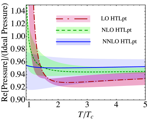
Figure 5: Comparison of LO, NLO, and NNLO predictions for the scaled real part of the pressure using the variational mass prescription. Shaded bands show the result of varying the renormalization scale $\mu$ by a factor of two around $\mu=2\pi T$.

In Fig. 5, we compare the LO, NLO, and NNLO predictions for the real part of the pressure normalized to that of an ideal gas. Shaded bands show the result of varying the renormalization scale $\mu$ by a factor of two around $\mu=2\pi T$. We use three-loop running of $\alpha_{s}$.

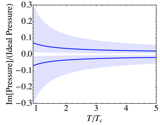
Figure 6: The NNLO result for the scaled imaginary part of the pressure with three-loop running and variational mass prescription. The two curves arise from the two complex conjugate solutions to the gap equations. Shaded bands show the result of varying the renormalization scale $\mu$ by a factor of two around $\mu=2\pi T$.

In Fig. 6, we show the NNLO result for the imaginary part of the pressure normalized by the ideal gas pressure. We use three-loop running of $\alpha_{s}$. The imaginary part decreases with increasing temperature and is rather small beyond 3-4 $T_{c}$.

5.2.2 BN mass

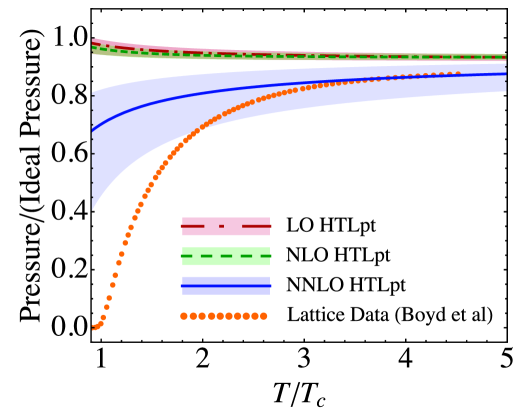
Figure 7: Comparison of LO, NLO, and NNLO predictions for the scaled pressure using the BN mass prescription and one-loop running of $\alpha_{s}$. The points are lattice data for pure-glue with $N_{c}=3$ from Boyd et al. [28]. Shaded bands show the result of varying the renormalization scale $\mu$ by a factor of two around $\mu=2\pi T$.

In Fig. 7, we show the HTLpt predictions for the pressure normalized to that of an ideal gas using the BN mass prescription. The bands are obtained by varying the renormalization scale by a factor of two around $\mu=2\pi T$. We use one-loop running of $\alpha_{s}$. In Fig. 8, we again plot the normalized pressure, but now with three-loop running of $\alpha_{s}$. The agreement between the lattice data from Boyd et al. [28] is very good down to temperatures of around 3 $T_{c}$. Comparing Figs. 7–8 we see that using the three-loop running, the band becomes wider. However, the difference is significant only for low $T$, where the HTLpt results disagrees with the lattice anyway. For $T>3T_{c}$, the prescription for the running makes very little difference.

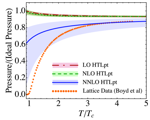
Figure 8: Comparison of LO, NLO, and NNLO predictions for the scaled pressure using the BN mass prescription and three-loop running of $\alpha_{s}$. The points are lattice data pure-glue with $N_{c}=3$ from Boyd et al. [28]. Shaded bands show the result of varying the renormalization scale $\mu$ by a factor of two around $\mu=2\pi T$.

Until recently, lattice data for thermodynamic variables only existed for temperatures up to approximately 5 $T_{c}$. In the paper by Enrodi et al [29], the authors calculate the pressure on the lattice for pure-glue QCD at very large temperatures. In Fig. 9, we show the results of Enrodi et al as well as Boyd et al, together with the HTLpt NLO and NNLO predictions for the pressure. The two points from Ref. [29] have large error bars, but the data points are consistent with the HTL predictions.

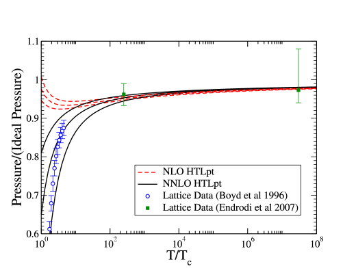
Figure 9: Comparison of NLO, and NNLO predictions for the scaled pressure with SU(3) pure-glue lattice data from Boyd et al. [28] and Endrodi et al. [29]. Shaded bands show the result of varying the renormalization scale $\mu$ by a factor of two around $\mu=2\pi T$.

We note that our prediction for the normalized free energy using either the leading-order, BN, or variational mass prescriptions is independent of $N_{c}$ if one holds $\alpha_{s}N_{c}$ fixed (’t Hooft limit). However, this need not be the case for an arbitrary mass prescription. The $N_{c}$-independence of the normalized free energy of the free energy is in agreement with recent lattice measurements that show a very small dependence of the free energy on $N_{c}$ [30, 31].

Due to the imaginary parts we do not show results coming from the variational prescription in the remainder of the results section. We will return to a discussion of the dependence on mass prescriptions in the conclusions.

5.3 Energy density

The energy density $\cal E$ is defined by

$${\cal E} = {\cal F}-T{d{\cal F}\over dT}\;.$$ (73)

In Fig. 10, we show the LO, NLO, and NNLO predictions for energy density normalized to that of an ideal gas. We use three-loop running and the BN mass. The bands show the result of varying the renormalization scale $\mu$ by a factor of two around $\mu=2\pi T$. Our NNLO predictions are in excellent agreement with the lattice data down to $T\simeq 2T_{c}$.

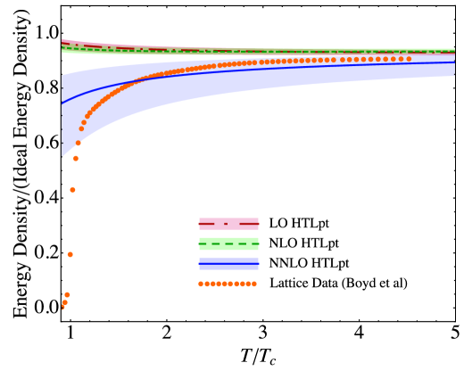
Figure 10: Comparison of LO, NLO, and NNLO predictions for the scaled energy density with SU(3) pure-glue lattice data from Boyd et al. [28]. We use three-loop running and the BN mass. Shaded bands show the result of varying the renormalization scale $\mu$ by a factor of two around $\mu=2\pi T$.

5.4 Entropy

The entropy density is defined by

$${\cal S} = -{\partial{\cal F}\over\partial T}\;,$$ (74)

where all other parameters that ${\cal F}$ depends on, are kept fixed. In Fig. 11, we show the entropy density normalized to that of an ideal gas. We use three-loop running and the BN mass. The points are lattice data from Boyd et al. [28]. Our NNLO predictions are in excellent agreement with the lattice data down to $T\simeq 2T_{c}$.

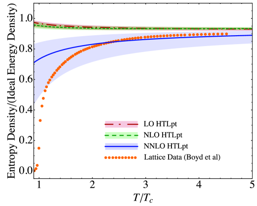
Figure 11: Comparison of LO, NLO, and NNLO predictions for the scaled entropy with SU(3) pure-glue lattice data from Boyd et al. [28]. We use three-loop running and the BN mass. Shaded bands show the result of varying the renormalization scale $\mu$ by a factor of two around $\mu=2\pi T$.

5.5 Trace anomaly

In pure-glue QCD or in QCD with massless quarks, there is no mass scale in the Lagrangian and the theory is scale invariant. At the classical level, this implies that the trace of the energy-momentum tensor vanishes. At the quantum level, scale invariance is broken by renormalization effects. It is convenient to introduce the scale anomaly density ${\cal E}-3{\cal P}$, which is proportional to the trace of the energy-momentum tensor. The trace anomaly can be written as

$${\cal E}-3{\cal P} = -T^{5}{d\over dT}\left({{\cal F}\over T^{4}}\right)\;.$$ (75)

In Fig. 12, we show the HTLpt predictions for the trace anomaly divided by ${\cal E}_{\rm ideal}$ using the BN mass prescription and three-loop running of $\alpha_{s}$. The points are lattice data from Boyd et al. [28] For temperatures below approximately 2$T_{c}$, there is a large discrepancy between the HTLpt predictions and lattice data. At LO and NLO, the curves are even bending downwards.

At temperatures close to the phase transition it has been suggested that the discrepancy between HTLpt resummed predictions for thermodynamics functions and, in particular, the trace anomaly is due to influence of a power corrections [32, 33, 34, 35, 36] which are related to confinement. Phenomenological fits of lattice data which include such power corrections show that the agreement with lattice data is improved [37, 38]. Alternatively, others have constructed AdS/CFT inspired models which break conformal invariance “by hand” [39, 40, 41, 42]. These models are also able to fit the thermodynamical functions of QCD at temperatures close to the phase transition.

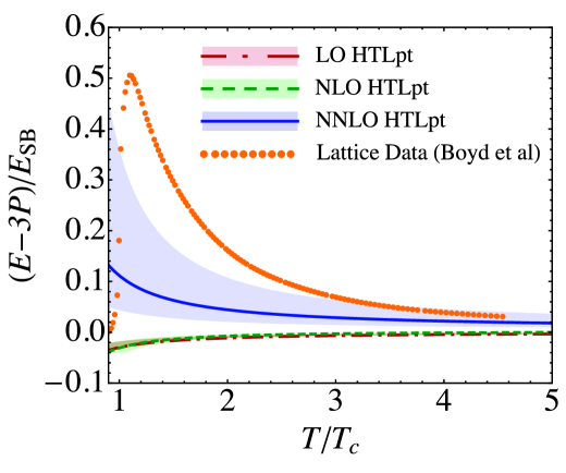
Figure 12: Comparison of LO, NLO, and NNLO predictions for the scaled trace anomaly with SU(3) pure-glue lattice data from Boyd et al. [28]. Shaded bands show the result of varying the renormalization scale $\mu$ by a factor of two around $\mu=2\pi T$.

In Fig. 13, we show the HTLpt predictions for the trace anomaly scaled by $T^{2}/T_{c}^{2}$ using the BN mass prescription and three-loop running of $\alpha_{s}$. The points are lattice data from Boyd et al. [28]. The most remarkable feature is that lattice data are essentially constant over a very large temperature range. Clearly, HTLpt does not reproduce the scaled lattice data precisely; however, the agreement is dramatically improved when going from NLO to NNLO.

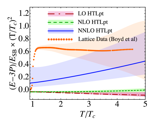
Figure 13: Comparison of LO, NLO, and NNLO predictions for the scaled trace anomaly multiplied by $T^{2}/T_{c}^{2}$ with SU(3) pure-glue lattice data from Boyd et al. [28]. Shaded bands show the result of varying the renormalization scale $\mu$ by a factor of two around $\mu=2\pi T$. Orange band shown with lattice data indicates scaled error assuming a $\pm 2.5\%$ error in the lattice data for the trace anomaly.

6 Conclusions

In this paper, we have presented results for the LO, NLO, and NNLO thermodynamic functions for SU($N_{c}$) Yang-Mills theory using HTLpt. We compared our predictions with lattice data for $N_{c}=3$ and found that with a perturbative mass prescription HTLpt is consistent with available lattice data down to approximately $T\sim 3\,T_{c}$ in the case of the pressure and $T\sim 2\,T_{c}$ in the case of the energy density and entropy. These results are in line with expectations since below $T\sim 2-3\,T_{c}$ a simple “electric” quasiparticle approximation breaks down due to nonperturbative chromomagnetic effects.

The mass parameter $m_{D}$ in HTLpt is arbitrary and we employed two different prescriptions for fixing it. Unfortunately, the variational gap equation has four complex conjugate solutions, two with positive real parts. This has also been observed in scalar theory and QED. Whether this is a problem of HTLpt as such or is related to our $m_{D}/T$ expansion is unknown. Since it is not currently possible to evaluate the NNLO HTLpt diagrams in gauge theories exactly, it is impossible to settle the issue at this stage. On the other hand, the BN mass prescription is well defined to all orders in perturbation theory and does a reasonable job reproducing available lattice data for temperatures above $T\simeq 3T_{c}$.

That being said without lattice data to compare with one would be hard pressed to favor one prescription over the other. While it is true that variational solutions are complex, one could be tempted to ignore the imaginary contributions and take ${\rm Re}[{\cal P}]$ as the approximation. As we have shown (see Fig. 5) in this case the convergence of HTLpt is impressive; however, the result lies above the lattice data at low temperatures. Taking the BN mass prescription on the other hand results in a real-valued pressure which seems to be in better agreement with the lattice data at the expense of poorer convergence of the successive approximations. The dependence on the mass prescription gives another measure of our theoretical uncertainty. If one were able to carry the HTLpt $\delta$ expansion to higher and higher orders the dependence on the mass prescription would go away; however, going to higher orders presents a rather daunting task since one encounters a purely non-perturbative contribution at ${\cal O}(\alpha_{s}^{3})$ for which lattice input is required.

Finally, we emphasize that HTLpt is gauge invariant by construction and that it can be used to calculate time-dependent quantities as well since it is formulated in Minkowski space. The fact that our BN mass results are consistent with lattice data down to approximately $3T_{c}$, suggests that HTLpt can provide a coherent framework that can be used to systematically calculate real-time quantities such as heavy quark diffusion and viscosity at temperatures relevant for LHC.

Appendix A HTL Feynman rules

In this appendix, we present Feynman rules for HTL perturbation theory in QCD. We give explicit expressions for the propagators and for the 3- and 4-gluon vertices. The Feynman rules are given in Minkowski space to facilitate future application to real-time processes. A Minkowski momentum is denoted $p=(p_{0},{\bf p})$, and the inner product is $p\cdot q=p_{0}q_{0}-{\bf p}\cdot{\bf q}$. The vector that specifies the thermal rest frame is $n=(1,{\bf 0})$.

A.1 Gluon self-energy

The HTL gluon self-energy tensor for a gluon of momentum $p$ is

$$\Pi^{\mu\nu}(p)=m_{D}^{2}\left[{\cal T}^{\mu\nu}(p,-p)-n^{\mu}n^{\nu}\right]\;.$$ (1)

The tensor ${\cal T}^{\mu\nu}(p,q)$, which is defined only for momenta that satisfy $p+q=0$, is

$${\cal T}^{\mu\nu}(p,-p)=\left\langle y^{\mu}y^{\nu}{p\!\cdot\!n\over p\!\cdot\!y}\right\rangle_{\bf\hat{y}}\;.$$ (2)

The angular brackets indicate averaging over the spatial directions of the light-like vector $y=(1,\hat{\bf y})$. The tensor ${\cal T}^{\mu\nu}$ is symmetric in $\mu$ and $\nu$ and satisfies the “Ward identity”

$$p_{\mu}{\cal T}^{\mu\nu}(p,-p)=p\!\cdot\!n\;n^{\nu}\;.$$ (3)

The self-energy tensor $\Pi^{\mu\nu}$ is therefore also symmetric in $\mu$ and $\nu$ and satisfies

$$p_{\mu}\Pi^{\mu\nu}(p) = 0\;,$$ (4)

$$g_{\mu\nu}\Pi^{\mu\nu}(p) = -m_{D}^{2}\;.$$ (5)

The gluon self-energy tensor can be expressed in terms of two scalar functions, the transverse and longitudinal self-energies $\Pi_{T}$ and $\Pi_{L}$, defined by

$$\Pi_{T}(p) = {1\over d-1}\left(\delta^{ij}-\hat{p}^{i}\hat{p}^{j}\right)\Pi^{ij}(p)\;,$$ (6)

$$\Pi_{L}(p) = -\Pi^{00}(p)\;,$$ (7)

where ${\bf\hat{p}}$ is the unit vector in the direction of ${\bf p}$. In terms of these functions, the self-energy tensor is

$$\Pi^{\mu\nu}(p)\;=\;-\Pi_{T}(p)T_{p}^{\mu\nu}-{1\over n_{p}^{2}}\Pi_{L}(p)L_{p}^{\mu\nu}\;,$$ (8)

where the tensors $T_{p}$ and $L_{p}$ are

$$T_{p}^{\mu\nu} = g^{\mu\nu}-{p^{\mu}p^{\nu}\over p^{2}}-{n_{p}^{\mu}n_{p}^{\nu}\over n_{p}^{2}}\;,$$ (9)

$$L_{p}^{\mu\nu} = {n_{p}^{\mu}n_{p}^{\nu}\over n_{p}^{2}}\;.$$ (10)

The four-vector $n_{p}^{\mu}$ is

$$n_{p}^{\mu}\;=\;n^{\mu}-{n\!\cdot\!p\over p^{2}}p^{\mu}\,,$$ (11)

and satisfies $p\!\cdot\!n_{p}=0$ and $n^{2}_{p}=1-(n\!\cdot\!p)^{2}/p^{2}$. The equation (5) reduces to the identity

$$(d-1)\Pi_{T}(p)+{1\over n^{2}_{p}}\Pi_{L}(p)\;=\;m_{D}^{2}\;.$$ (12)

We can express both self-energy functions in terms of the function ${\cal T}^{00}$ defined by (2):

$$\Pi_{T}(p) = {m_{D}^{2}\over(d-1)n_{p}^{2}}\left[{\cal T}^{00}(p,-p)-1+n_{p}^{2}\right],$$ (13)

$$\Pi_{L}(p) = m_{D}^{2}\left[1-{\cal T}^{00}(p,-p)\right],$$ (14)

In the tensor ${\cal T}^{\mu\nu}(p,-p)$ defined in (2), the angular brackets indicate the angular average over the unit vector $\hat{\bf y}$. In almost all previous work, the angular average in (2) has been taken in $d=3$ dimensions. For consistency of higher-order corrections, it is essential to take the angular average in $d=3-2\epsilon$ dimensions and analytically continue to $d=3$ only after all poles in $\epsilon$ have been cancelled. Expressing the angular average as an integral over the cosine of an angle, the expression for the $00$ component of the tensor is

$$\!\!\!{\cal T}^{00}(p,-p)\!\! = \!\!{w(\epsilon)\over 2}\!\!\int_{-1}^{1}\!\!dc\;(1-c^{2})^{-\epsilon}{p_{0}\over p_{0}-|{\bf p}|c}\,,$$ (15)

where the weight function $w(\epsilon)$ is

$$w(\epsilon)={\Gamma(2-2\epsilon)\over\Gamma^{2}(1-\epsilon)}2^{2\epsilon}={\Gamma({3\over 2}-\epsilon)\over\Gamma({3\over 2})\Gamma(1-\epsilon)}\;.$$ (16)

The integral in (15) must be defined so that it is analytic at $p_{0}=\infty$. It then has a branch cut running from $p_{0}=-|{\bf p}|$ to $p_{0}=+|{\bf p}|$. If we take the limit $\epsilon\rightarrow 0$, it reduces to

$${\cal T}^{00}(p,-p) = {p_{0}\over 2|{\bf p}|}\log{p_{0}+|{\bf p}|\over p_{0}-|{\bf p}|}\;,$$ (17)

which is the expression that appears in the usual HTL self-energy functions.

A.2 Gluon propagator

The Feynman rule for the gluon propagator is

$$i\delta^{ab}\Delta_{\mu\nu}(p)\;,$$ (18)

where the gluon propagator tensor $\Delta_{\mu\nu}$ depends on the choice of gauge fixing. We consider two possibilities that introduce an arbitrary gauge parameter $\xi$: general covariant gauge and general Coulomb gauge. In both cases, the inverse propagator reduces in the limit $\xi\rightarrow\infty$ to

$$\Delta^{-1}_{\infty}(p)^{\mu\nu} = -p^{2}g^{\mu\nu}+p^{\mu}p^{\nu}-\Pi^{\mu\nu}(p)\;.$$ (19)

This can also be written

$$\Delta^{-1}_{\infty}(p)^{\mu\nu} = -{1\over\Delta_{T}(p)}T_{p}^{\mu\nu}+{1\over n_{p}^{2}\Delta_{L}(p)}L_{p}^{\mu\nu}\;,$$ (20)

where $\Delta_{T}$ and $\Delta_{L}$ are the transverse and longitudinal propagators:

$$\Delta_{T}(p) = {1\over p^{2}-\Pi_{T}(p)}\;,$$ (21)

$$\Delta_{L}(p) = {1\over-n_{p}^{2}p^{2}+\Pi_{L}(p)}\;.$$ (22)

The inverse propagator for general $\xi$ is

$$\Delta^{-1}(p)^{\mu\nu} = \Delta^{-1}_{\infty}(p)^{\mu\nu}-{1\over\xi}p^{\mu}p^{\nu}\hskip 5.69046pt\mbox{covariant}\;,$$ (24)

$$= \Delta^{-1}_{\infty}(p)^{\mu\nu}-{1\over\xi}\left(p^{\mu}-p\!\cdot\!n\;n^{\mu}\right)\left(p^{\nu}-p\!\cdot\!n\;n^{\nu}\right)$$

$$\hskip 105.2751pt\mbox{Coulomb}\;.$$

The propagators obtained by inverting the tensors in (24) and (24) are

$$\Delta^{\mu\nu}(p) = -\Delta_{T}(p)T_{p}^{\mu\nu}+\Delta_{L}(p)n_{p}^{\mu}n_{p}^{\nu}-\xi{p^{\mu}p^{\nu}\over(p^{2})^{2}}$$ (26)

$$\hskip 105.2751pt\mbox{covariant}\;,$$

$$= -\Delta_{T}(p)T_{p}^{\mu\nu}+\Delta_{L}(p)n^{\mu}n^{\nu}-\xi{p^{\mu}p^{\nu}\over\left(n_{p}^{2}p^{2}\right)^{2}}$$

$$\hskip 105.2751pt\mbox{Coulomb}\;.$$

It is convenient to define the following combination of propagators:

$$\Delta_{X}(p) = \Delta_{L}(p)+{1\over n_{p}^{2}}\Delta_{T}(p)\;.$$ (27)

Using (12), (21), and (22), it can be expressed in the alternative form

$$\Delta_{X}(p) = \left[m_{D}^{2}-d\,\Pi_{T}(p)\right]\Delta_{L}(p)\Delta_{T}(p)\;,$$ (28)

which shows that it vanishes in the limit $m_{D}\to 0$. In the covariant gauge, the propagator tensor can be written

$$\Delta^{\mu\nu}(p) = \left[-\Delta_{T}(p)g^{\mu\nu}+\Delta_{X}(p)n^{\mu}n^{\nu}\right]-{n\!\cdot\!p\over p^{2}}\Delta_{X}(p)\left(p^{\mu}n^{\nu}+n^{\mu}p^{\nu}\right)$$

$$+\left[\Delta_{T}(p)+{(n\!\cdot\!p)^{2}\over p^{2}}\Delta_{X}(p)-{\xi\over p^{2}}\right]{p^{\mu}p^{\nu}\over p^{2}}\;.$$

This decomposition of the propagator into three terms has proved to be particularly convenient for explicit calculations. For example, the first term satisfies the identity

$$\left[-\Delta_{T}(p)g_{\mu\nu}+\Delta_{X}(p)n_{\mu}n_{\nu}\right]\Delta^{-1}_{\infty}(p)^{\nu\lambda} = {g_{\mu}}^{\lambda}-{p_{\mu}p^{\lambda}\over p^{2}}+{n\!\cdot\!p\over n_{p}^{2}p^{2}}{\Delta_{X}(p)\over\Delta_{L}(p)}p_{\mu}n_{p}^{\lambda}\;.$$ (30)

A.3 Three-gluon vertex

The three-gluon vertex for gluons with outgoing momenta $p$, $q$, and $r$, Lorentz indices $\mu$, $\nu$, and $\lambda$, and color indices $a$, $b$, and $c$ is

$$i\Gamma_{abc}^{\mu\nu\lambda}(p,q,r)=-gf_{abc}\Gamma^{\mu\nu\lambda}(p,q,r)\;,$$ (31)

where $f^{abc}$ are the structure constants and the three-gluon vertex tensor is

$$\Gamma^{\mu\nu\lambda}(p,q,r) = g^{\mu\nu}(p-q)^{\lambda}+g^{\nu\lambda}(q-r)^{\mu}+g^{\lambda\mu}(r-p)^{\nu}-m_{D}^{2}{\cal T}^{\mu\nu\lambda}(p,q,r)\;.$$ (32)

The tensor ${\cal T}^{\mu\nu\lambda}$ in the HTL correction term is defined only for $p+q+r=0$:

$${\cal T}^{\mu\nu\lambda}(p,q,r)\;=\;-\Bigg{\langle}y^{\mu}y^{\nu}y^{\lambda}\left({p\!\cdot\!n\over p\!\cdot\!y\;q\!\cdot\!y}-{r\!\cdot\!n\over\!r\cdot\!y\;q\!\cdot\!y}\right)\Bigg{\rangle}\;.$$ (33)

This tensor is totally symmetric in its three indices and traceless in any pair of indices: $g_{\mu\nu}{\cal T}^{\mu\nu\lambda}=0$. It is odd (even) under odd (even) permutations of the momenta $p$, $q$, and $r$. It satisfies the “Ward identity”

$$q_{\mu}{\cal T}^{\mu\nu\lambda}(p,q,r)\;=\;{\cal T}^{\nu\lambda}(p+q,r)-{\cal T}^{\nu\lambda}(p,r+q)\;.$$ (34)

The three-gluon vertex tensor therefore satisfies the Ward identity

$$p_{\mu}\Gamma^{\mu\nu\lambda}(p,q,r)\;=\;\Delta_{\infty}^{-1}(q)^{\nu\lambda}-\Delta_{\infty}^{-1}(r)^{\nu\lambda}\;.$$ (35)

A.4 Four-gluon vertex

The four-gluon vertex for gluons with outgoing momenta $p$, $q$, $r$, and $s$, Lorentz indices $\mu$, $\nu$, $\lambda$, and $\sigma$, and color indices $a$, $b$, $c$, and $d$ is

$$i\Gamma^{\mu\nu\lambda\sigma}_{abcd}(p,q,r,s) = -ig^{2}\big{\{}f_{abx}f_{xcd}\left(g^{\mu\lambda}g^{\nu\sigma}-g^{\mu\sigma}g^{\nu\lambda}\right)$$ (36)

$$+2m_{D}^{2}\mbox{tr}\left[T^{a}\left(T^{b}T^{c}T^{d}+T^{d}T^{c}T^{b}\right)\right]{\cal T}^{\mu\nu\lambda\sigma}(p,q,r,s)\big{\}}$$

$$+\;2\;\mbox{cyclic permutations}\;,$$

where the cyclic permutations are of $(q,\nu,b)$, $(r,\lambda,c)$, and $(s,\sigma,d)$. The matrices $T^{a}$ are the fundamental representation of the $SU(3)$ algebra with the standard normalization ${\rm tr}(T^{a}T^{b})={1\over 2}\delta^{ab}$. The tensor ${\cal T}^{\mu\nu\lambda\sigma}$ in the HTL correction term is defined only for $p+q+r+s=0$:

$${\cal T}^{\mu\nu\lambda\sigma}(p,q,r,s) = \Bigg{\langle}y^{\mu}y^{\nu}y^{\lambda}y^{\sigma}\left({p\!\cdot\!n\over p\!\cdot\!y\;q\!\cdot\!y\;(q+r)\!\cdot\!y}\right.$$ (37)

$$\hskip 28.45274pt\left.+{(p+q)\!\cdot\!n\over q\!\cdot\!y\;r\!\cdot\!y\;(r+s)\!\cdot\!y}+{(p+q+r)\!\cdot\!n\over r\!\cdot\!y\;s\!\cdot\!y\;(s+p)\!\cdot\!y}\right)\Bigg{\rangle}\;.$$

This tensor is totally symmetric in its four indices and traceless in any pair of indices: $g_{\mu\nu}{\cal T}^{\mu\nu\lambda\sigma}=0$. It is even under cyclic or anti-cyclic permutations of the momenta $p$, $q$, $r$, and $s$. It satisfies the “Ward identity”

$$q_{\mu}{\cal T}^{\mu\nu\lambda\sigma}(p,q,r,s) = {\cal T}^{\nu\lambda\sigma}(p+q,r,s)$$ (38)

$$-{\cal T}^{\nu\lambda\sigma}(p,r+q,s)$$

and the “Bianchi identity”

$${\cal T}^{\mu\nu\lambda\sigma}(p,q,r,s)+{\cal T}^{\mu\nu\lambda\sigma}(p,r,s,q)+{\cal T}^{\mu\nu\lambda\sigma}(p,s,q,r)=0\;.$$

(39)

When its color indices are traced in pairs, the four-gluon vertex becomes particularly simple:

$$\delta^{ab}\delta^{cd}i\Gamma_{abcd}^{\mu\nu\lambda\sigma}(p,q,r,s) = -ig^{2}N_{c}(N_{c}^{2}-1)\Gamma^{\mu\nu,\lambda\sigma}(p,q,r,s)\;,$$ (40)

where the color-traced four-gluon vertex tensor is

$$\Gamma^{\mu\nu,\lambda\sigma}(p,q,r,s) = 2g^{\mu\nu}g^{\lambda\sigma}-g^{\mu\lambda}g^{\nu\sigma}-g^{\mu\sigma}g^{\nu\lambda}-m_{D}^{2}{\cal T}^{\mu\nu\lambda\sigma}(p,s,q,r)\;.$$ (41)

Note the ordering of the momenta in the arguments of the tensor ${\cal T}^{\mu\nu\lambda\sigma}$, which comes from the use of the Bianchi identity (39). The tensor (41) is symmetric under the interchange of $\mu$ and $\nu$, under the interchange of $\lambda$ and $\sigma$, and under the interchange of $(\mu,\nu)$ and $(\lambda,\sigma)$. It is also symmetric under the interchange of $p$ and $q$, under the interchange of $r$ and $s$, and under the interchange of $(p,q)$ and $(r,s)$. It satisfies the Ward identity

$$p_{\mu}\Gamma^{\mu\nu,\lambda\sigma}(p,q,r,s) = \Gamma^{\nu\lambda\sigma}(q,r+p,s)-\Gamma^{\nu\lambda\sigma}(q,r,s+p)\;.$$ (42)

A.5 Ghost propagator and vertex

The ghost propagator and the ghost-gluon vertex depend on the gauge. The Feynman rule for the ghost propagator is

$${i\over p^{2}}\delta^{ab}\hskip 71.13188pt\mbox{covariant}\;,$$ (43)

$${i\over n_{p}^{2}p^{2}}\delta^{ab}\hskip 56.9055pt\mbox{Coulomb}\;.$$ (44)

The Feynman rule for the vertex in which a gluon with indices $\mu$ and $a$ interacts with an outgoing ghost with outgoing momentum $r$ and color index $c$ is

$$-gf^{abc}r^{\mu}\hskip 93.89418pt\mbox{covariant}\;,$$ (45)

$$-gf^{abc}\left(r^{\mu}-r\!\cdot\!n\;n^{\mu}\right)\hskip 28.45274pt\mbox{Coulomb}\;.$$ (46)

Every closed ghost loop requires a multiplicative factor of $-1$.

A.6 HTL counterterm

The Feynman rule for the insertion of an HTL counterterm into a gluon propagator is

$$-i\delta^{ab}\Pi^{\mu\nu}(p)\;,$$ (47)

where $\Pi^{\mu\nu}(p)$ is the HTL gluon self-energy tensor given in (8).

A.7 Imaginary-time formalism

In the imaginary-time formalism, Minkoswski energies have discrete imaginary values $p_{0}=i(2\pi nT)$ and integrals over Minkowski space are replaced by sum-integrals over Euclidean vectors $(2\pi nT,{\bf p})$. We will use the notation $P=(P_{0},{\bf p})$ for Euclidean momenta. The magnitude of the spatial momentum will be denoted $p=|{\bf p}|$, and should not be confused with a Minkowski vector. The inner product of two Euclidean vectors is $P\cdot Q=P_{0}Q_{0}+{\bf p}\cdot{\bf q}$. The vector that specifies the thermal rest frame remains $n=(1,{\bf 0})$.

The Feynman rules for Minkowski space given above can be easily adapted to Euclidean space. The Euclidean tensor in a given Feynman rule is obtained from the corresponding Minkowski tensor with raised indices by replacing each Minkowski energy $p_{0}$ by $iP_{0}$, where $P_{0}$ is the corresponding Euclidean energy, and multipying by $-i$ for every $0$ index. This prescription transforms $p=(p_{0},{\bf p})$ into $P=(P_{0},{\bf p})$, $g^{\mu\nu}$ into $-\delta^{\mu\nu}$, and $p\!\cdot\!q$ into $-P\!\cdot\!Q$. The effect on the HTL tensors defined in (2), (33), and (37) is equivalent to substituting $p\!\cdot\!n\to-P\!\cdot\!N$ where $N=(-i,{\bf 0})$, $p\!\cdot\!y\to-P\!\cdot\!Y$ where $Y=(-i,{\bf\hat{y}})$, and $y^{\mu}\to Y^{\mu}$. For example, the Euclidean tensor corresponding to (2) is

$${\cal T}^{\mu\nu}(P,-P)=\left\langle Y^{\mu}Y^{\nu}{P\!\cdot\!N\over P\!\cdot\!Y}\right\rangle\;.$$ (48)

The average is taken over the directions of the unit vector ${\bf\hat{y}}$.

Alternatively, one can calculate a diagram by using the Feynman rules for Minkowski momenta, reducing the expressions for diagrams to scalars, and then make the appropriate substitutions, such as $p^{2}\to-P^{2}$, $p\cdot q\to-P\cdot Q$, and $n\cdot p\to in\cdot P$. For example, the propagator functions (21) and (22) become

$$\Delta_{T}(P) = {-1\over P^{2}+\Pi_{T}(P)}\;,$$ (49)

$$\Delta_{L}(P) = {1\over p^{2}+\Pi_{L}(P)}\;.$$ (50)

The expressions for the HTL self-energy functions $\Pi_{T}(P)$ and $\Pi_{L}(P)$ are given by (13) and (14) with $n_{p}^{2}$ replaced by $n_{P}^{2}=p^{2}/P^{2}$ and ${\cal T}^{00}(p,-p)$ replaced by

$${\cal T}_{P} = {w(\epsilon)\over 2}\int_{-1}^{1}dc\;(1-c^{2})^{-\epsilon}{iP_{0}\over iP_{0}-pc}\;.$$ (51)

Note that this function differs by a sign from the 00 component of the Euclidean tensor corresponding to (2):

$${\cal T}^{00}(P,-P)=-{\cal T}^{00}(p,-p)\bigg{|}_{p_{0}\to iP_{0}}=-{\cal T}_{P}\;.$$ (52)

A more convenient form for calculating sum-integrals that involve the function ${\cal T}_{P}$ is

$${\cal T}_{P} = \left\langle{P_{0}^{2}\over P_{0}^{2}+p^{2}c^{2}}\right\rangle_{\!\!c}\,,$$ (53)

where the angular brackets represent an average over $c$ defined by

$$\left\langle f(c)\right\rangle_{\!c}\equiv w(\epsilon)\int_{0}^{1}dc\,(1-c^{2})^{-\epsilon}f(c)\,,$$ (54)

and $w(\epsilon)$ is given in (16).

Appendix B Sum-integrals

In the imaginary-time formalism for thermal field theory, the 4-momentum $P=(P_{0},{\bf p})$ is Euclidean with $P^{2}=P_{0}^{2}+{\bf p}^{2}$. The Euclidean energy $P_{0}$ has discrete values: $P_{0}=2n\pi T$ for bosons, where $n$ is an integer. Loop diagrams involve sums over $P_{0}$ and integrals over ${\bf p}$. With dimensional regularization, the integral is generalized to $d=3-2\epsilon$ spatial dimensions. We define the dimensionally regularized sum-integral by

$$\hbox{$\sum$}\!\!\!\!\!\!\int_{P} \equiv \left(\frac{e^{\gamma_{E}}\mu^{2}}{4\pi}\right)^{\epsilon}\;T\sum_{P_{0}=2n\pi T}\>\int{d^{3-2\epsilon}p\over(2\pi)^{3-2\epsilon}}\;,$$ (1)

where $3-2\epsilon$ is the dimension of space and $\mu$ is an arbitrary momentum scale. The factor $(e^{\gamma_{E}}/4\pi)^{\epsilon}$ is introduced so that, after minimal subtraction of the poles in $\epsilon$ due to ultraviolet divergences, $\mu$ coincides with the renormalization scale of the $\overline{\rm MS}$ renormalization scheme.

Below we list the sum-integrals required to complete the three loop calculation. We refer to Ref. [18] for details concerning the sum-integral evaluations.

B.1 One-loop sum-integrals

The simple one-loop sum-integrals required in our calculations can be derived from the formulas

$$\hbox{$\sum$}\!\!\!\!\!\!\!\int_{P}{p^{2m}\over(P^{2})^{n}}\!\! = \!\!\left({\mu\over 4\pi T}\right)^{2\epsilon}{2\Gamma({3\over 2}+m-\epsilon)\Gamma(n-{3\over 2}-m+\epsilon)\over\Gamma(n)\Gamma(2-2\epsilon)}$$ (2)

$$\;\times\,\Gamma(1-\epsilon)\zeta(2n-2m-3+2\epsilon)e^{\epsilon\gamma_{E}}$$

$$\;\;\;\;\times\,T^{4+2m-2n}(2\pi)^{1+2m-2n}\;.$$

The specific bosonic one-loop sum-integrals needed are

$$\hbox{$\sum$}\!\!\!\!\!\!\!\int_{P}\log P^{2} = -{\pi^{2}\over 45}T^{4}\;,$$ (3)

$$\hbox{$\sum$}\!\!\!\!\!\!\!\int_{P}{1\over P^{2}} = {T^{2}\over 12}\left({\mu\over 4\pi T}\right)^{2\epsilon}\Bigg{[}1+\left(2+2{\zeta^{\prime}(-1)\over\zeta(-1)}\right)\epsilon+{\cal O}(\epsilon^{2})\Bigg{]}\;,$$ (4)

$$\hbox{$\sum$}\!\!\!\!\!\!\!\int_{P}{1\over(P^{2})^{2}} = {1\over(4\pi)^{2}}\left({\mu\over 4\pi T}\right)^{2\epsilon}\left[{1\over\epsilon}+2\gamma_{E}+{\cal O}(\epsilon)\right]\;,$$ (5)

$$\hbox{$\sum$}\!\!\!\!\!\!\!\int_{P}{1\over p^{2}P^{2}} = {1\over(4\pi)^{2}}\left({\mu\over 4\pi T}\right)^{2\epsilon}2\left[{1\over\epsilon}+2\gamma_{E}+2+{\cal O}(\epsilon)\right]\;.$$ (6)

The number $\gamma_{1}$ is the first Stieltjes gamma constant defined by the equation

$$\zeta(1+z)={1\over z}+\gamma_{E}-\gamma_{1}z+O(z^{2})\;.$$ (7)

We also need some more difficult one-loop sum-integrals that involve the HTL function defined in (51). The specific bosonic sum-integrals needed are

$$\hbox{$\sum$}\!\!\!\!\!\!\!\int_{P}{1\over p^{4}}{\cal T}_{P} = {1\over(4\pi)^{2}}\left({\mu\over 4\pi T}\right)^{2\epsilon}(-1)\left[{1\over\epsilon}+2\gamma_{E}+2\log 2+{\cal O}(\epsilon)\right]\;,$$ (8)

$$\hbox{$\sum$}\!\!\!\!\!\!\!\int_{P}{1\over p^{2}P^{2}}{\cal T}_{P} = {1\over(4\pi)^{2}}\left({\mu\over 4\pi T}\right)^{2\epsilon}\bigg{[}2\log 2\left({1\over\epsilon}+2\gamma_{E}\right)+2\log^{2}2+{\pi^{2}\over 3}+{\cal O}(\epsilon)\bigg{]}\;,$$ (9)

$$\hbox{$\sum$}\!\!\!\!\!\!\!\int_{P}{1\over p^{4}}({\cal T}_{P})^{2} = {1\over(4\pi)^{2}}\left({\mu\over 4\pi T}\right)^{2\epsilon}\left(-{2\over 3}\right)\left[(1+2\log 2)\left({1\over\epsilon}+2\gamma_{E}\right)-{4\over 3}+{22\over 3}\log 2+2\log^{2}2+{\cal O}(\epsilon)\right]\;.$$

B.2 Two-loop sum-integrals

The simple two-loop sum-integrals that are needed are

$$\hbox{$\sum$}\!\!\!\!\!\!\!\int_{PQ}{1\over P^{2}Q^{2}R^{2}} = {\cal O}(\epsilon)\,,$$ (11)

$$\hbox{$\sum$}\!\!\!\!\!\!\!\int_{PQ}{1\over P^{2}Q^{2}r^{2}} = {T^{2}\over(4\pi)^{2}}\left({\mu\over 4\pi T}\right)^{4\epsilon}{1\over 12}\left[{1\over\epsilon}+10-12\log 2+4{\zeta^{\prime}(-1)\over\zeta(-1)}+{\cal O}(\epsilon)\right]\,,$$ (12)

$$\hbox{$\sum$}\!\!\!\!\!\!\!\int_{PQ}{q^{2}\over P^{2}Q^{2}r^{4}} = {T^{2}\over(4\pi)^{2}}\left({\mu\over 4\pi T}\right)^{4\epsilon}{1\over 6}\left[{1\over\epsilon}+{8\over 3}+2\gamma_{E}+2{\zeta^{\prime}(-1)\over\zeta(-1)}+{\cal O}(\epsilon)\right]\,,$$ (13)

$$\hbox{$\sum$}\!\!\!\!\!\!\!\int_{PQ}{q^{2}\over P^{2}Q^{2}r^{2}R^{2}} = {T^{2}\over(4\pi)^{2}}\left({\mu\over 4\pi T}\right)^{4\epsilon}{1\over 9}\left[{1\over\epsilon}+7.521+{\cal O}(\epsilon)\right]\,,$$ (14)

$$\hbox{$\sum$}\!\!\!\!\!\!\!\int_{PQ}{P\!\cdot\!Q\over P^{2}Q^{2}r^{4}} = {T^{2}\over(4\pi)^{2}}\left({\mu\over 4\pi T}\right)^{4\epsilon}\left(-{1\over 8}\right)\left[{1\over\epsilon}+{2\over 9}+4\log 2+{8\over 3}\gamma_{E}+{4\over 3}{\zeta^{\prime}(-1)\over\zeta(-1)}+{\cal O}(\epsilon)\right]\,,$$

where $R=-(P+Q)$ and $r=|{\bf p}+{\bf q}|$. We also need some more difficult two-loop sum-integrals that involve the functions ${\cal T}_{P}$ defined in (51). The specific bosonic sum-integrals needed are

$$\hbox{$\sum$}\!\!\!\!\!\!\!\int_{PQ}{1\over P^{2}Q^{2}r^{2}}{\cal T}_{R} = {T^{2}\over(4\pi)^{2}}\left({\mu\over 4\pi T}\right)^{4\epsilon}\left(-{1\over 48}\right)\left[{1\over\epsilon^{2}}\right.\left.\;+\;\left(2-12\log 2+4{\zeta^{\prime}(-1)\over\zeta(-1)}\right){1\over\epsilon}\right.$$ (16)

$$\left.\hskip 113.81102pt-19.83+{\cal O}(\epsilon)\right]\,,$$

$$\hbox{$\sum$}\!\!\!\!\!\!\!\int_{PQ}{q^{2}\over P^{2}Q^{2}r^{4}}{\cal T}_{R} = {T^{2}\over(4\pi)^{2}}\left({\mu\over 4\pi T}\right)^{4\epsilon}\left(-{1\over 576}\right)\left[{1\over\epsilon^{2}}\right.\left.\;+\;\left({26\over 3}-{24\over\pi^{2}}-92\log 2+4{\zeta^{\prime}(-1)\over\zeta(-1)}\right){1\over\epsilon}\right.$$ (17)

$$\left.\hskip 113.81102pt-477.7+{\cal O}(\epsilon)\right]\,,$$

$$\hbox{$\sum$}\!\!\!\!\!\!\!\int_{PQ}{P\!\cdot\!Q\over P^{2}Q^{2}r^{4}}{\cal T}_{R} = {T^{2}\over(4\pi)^{2}}\left({\mu\over 4\pi T}\right)^{4\epsilon}\left(-{1\over 96}\right)\left[{1\over\epsilon^{2}}\right.\left.\;+\;\left({8\over\pi^{2}}+4\log 2+4{\zeta^{\prime}(-1)\over\zeta(-1)}\right){1\over\epsilon}\right.$$ (18)

$$\left.\hskip 113.81102pt+59.66+{\cal O}(\epsilon)\right]\,.$$

B.3 Three-loop sum-integrals

The three-loop sum-integrals needed are

$$\hbox{$\sum$}\!\!\!\!\!\!\!\int_{PQR}{1\over P^{2}Q^{2}R^{2}(P+Q+R)^{2}} = {1\over 24(4\pi)^{2}}T^{4}\left({\mu\over 4\pi T}\right)^{6\epsilon}\left[{1\over\epsilon}+{91\over 15}+8{\zeta^{\prime}(-1)\over\zeta(-1)}\right.$$ (19)

$$\left.\hskip 56.9055pt-2{\zeta^{\prime}(-3)\over\zeta(-3)}+{\cal O}(\epsilon)\right]\;,$$

$$\hbox{$\sum$}\!\!\!\!\!\!\!\int_{PQR}{(P-Q)^{4}\over P^{2}Q^{2}R^{4}(Q-R)^{2}(R-P)^{2}} = {11\over 216(4\pi)^{2}}T^{4}\left({\mu\over 4\pi T}\right)^{6\epsilon}\left[{1\over\epsilon}+{73\over 22}+{12\over 11}\gamma_{E}+{64\over 11}{\zeta^{\prime}(-1)\over\zeta(-1)}\right.$$ (20)

$$\left.\hskip 56.9055pt-{10\over 11}{\zeta^{\prime}(-3)\over\zeta(-3)}+{\cal O}(\epsilon)\right]\;.$$

The three-loop sum-integrals were first calculated by Arnold and Zhai and calculational details can be found in Ref. [6].

Appendix C Three-dimensional integrals

Dimensional regularization can be used to regularize both the ultraviolet divergences and infrared divergences in 3-dimensional integrals over momenta. The spatial dimension is generalized to $d=3-2\epsilon$ dimensions. Integrals are evaluated at a value of $d$ for which they converge and then analytically continued to $d=3$. We use the integration measure

$$\int_{p}\;\equiv\;\left(\frac{e^{\gamma_{E}}\mu^{2}}{4\pi}\right)^{\epsilon}\;\>\int{d^{3-2\epsilon}p\over(2\pi)^{3-2\epsilon}}\;.$$ (21)

C.1 One-loop integrals

The one-loop integral is given by

$$I_{n} \equiv \int_{p}{1\over(p^{2}+m^{2})^{n}}$$ (22)

$$= {1\over 8\pi}(e^{\gamma_{E}}\mu^{2})^{\epsilon}{\Gamma(n-\mbox{$3\over 2$}+\epsilon)\over\Gamma(\mbox{$1\over 2$})\Gamma(n)}m^{3-2n-2\epsilon}\;.$$

Specifically, we need

$$I_{0}^{\prime} \equiv \int_{p}\log(p^{2}+m^{2})$$ (23)

$$= -{m^{3}\over 6\pi}\left({\mu\over 2m}\right)^{2\epsilon}\left[1+{8\over 3}\epsilon+{\cal O}\left(\epsilon^{2}\right)\right]\;,$$

$$I_{1} = -{m\over 4\pi}\left({\mu\over 2m}\right)^{2\epsilon}\left[1+2\epsilon+{\cal O}\left(\epsilon^{2}\right)\right]\;,$$ (24)

$$I_{2} = {1\over 8\pi m}\left({\mu\over 2m}\right)^{2\epsilon}\left[1+{\cal O}\left(\epsilon\right)\right]\;.$$ (25)

C.2 Two-loop integrals

We also need a few two-loop integrals on the form

$$J_{n} = \int_{pq}{1\over p^{2}+m^{2}}{1\over(q^{2}+m^{2})^{n}}{1\over({\bf p}+{\bf q})^{2}}\;,$$ (26)

$$K_{n} = \int_{pq}{1\over p^{2}+m^{2}}{1\over(q^{2}+m^{2})}{1\over[({\bf p}+{\bf q})^{2}]^{n}}\;.$$ (27)

Specifically, we need $J_{1}$, $J_{2}$, and $K_{1}$ which were calculated in Refs. [9, 11]:

$$J_{1} = {1\over 4(4\pi)^{2}}\left({\mu\over 2m}\right)^{4\epsilon}\left[{1\over\epsilon}+2+{\cal O}(\epsilon)\right]\;,$$ (28)

$$J_{2} = {1\over 4(4\pi)^{2}m^{2}}\left({\mu\over 2m}\right)^{4\epsilon}\left[1+{\cal O}(\epsilon)\right]\;,$$ (29)

$$K_{2} = -{1\over 8m^{2}(4\pi)^{2}}\left({\mu\over 2m}\right)^{4\epsilon}\left[1+{\cal O}(\epsilon)\right]\;.$$ (30)

C.3 Three-loop integrals

We also need a number of three-loop integrals. The specific integrals we need are listed below and were calculated in Refs. [9, 11]. They are special cases of more general integrals defined in Ref. [44].

$$\int_{pqr}{1\over(p^{2}+m^{2})(q^{2}+m^{2})}{1\over r^{2}({\bf p}+{\bf q}+{\bf r})^{2}} = -{m\over 2(4\pi)^{3}}\left({\mu\over 2m}\right)^{6\epsilon}$$ (31)

$$\times\left[{1\over\epsilon}+8+{\cal O}(\epsilon)\right]\;,$$

$$\int_{pqr}{(r^{2}+m^{2})\over(p^{2}+m^{2})(q^{2}+m^{2})}{1\over({\bf p}-{\bf q})^{2}({\bf q}-{\bf r})^{2}({\bf r}-{\bf p})^{2}} = {m\over 4(4\pi)^{3}}\left({\mu\over 2m}\right)^{6\epsilon}$$ (32)

$$\times\left[{1\over\epsilon}+8+{\cal O}(\epsilon)\right]\;,$$

$$\int_{pqr}{(r^{2}+m^{2})^{2}\over(p^{2}+m^{2})(q^{2}+m^{2})}{1\over({\bf p}-{\bf q})^{4}({\bf q}-{\bf r})^{2}({\bf r}-{\bf p})^{2}} = -{m\over 4(4\pi)^{3}}\left({\mu\over 2m}\right)^{6\epsilon}$$ (33)

$$\times\left[{1\over\epsilon}+6+{\cal O}(\epsilon)\right]\;,$$

$$\int_{pqr}{1\over(p^{2}+m^{2})(q^{2}+m^{2})(r^{2}+m^{2})}{1\over({\bf q}-{\bf r})^{2}({\bf r}-{\bf p})^{2}} = {1\over m(4\pi)^{3}}\left({\mu\over 2m}\right)^{6\epsilon}$$ (34)

$$\times\left[{\pi^{2}\over 12}+{\cal O}(\epsilon)\right]\;,$$

$$\int_{pqr}{1\over(p^{2}+m^{2})(q^{2}+m^{2})}{1\over({\bf p}-{\bf q})^{2}({\bf q}-{\bf r})^{2}({\bf r}-{\bf p})^{2}} = -{1\over 8m(4\pi)^{3}}\left({\mu\over 2m}\right)^{6\epsilon}$$ (35)

$$\times\left[{1\over\epsilon}-2+{\cal O}(\epsilon)\right]\;,$$

$$\int_{pqr}{1\over(p^{2}+m^{2})(q^{2}+m^{2})(r^{2}+m^{2})^{2}}{1\over({\bf q}-{\bf r})^{2}({\bf r}-{\bf p})^{2}} = -{1\over 4m^{3}(4\pi)^{3}}\left({\mu\over 2m}\right)^{6\epsilon}$$ (36)

$$\times\left[1-{\pi^{2}\over 6}+{\cal O}(\epsilon)\right]\;,$$

$$\int_{pqr}{1\over(p^{2}+m^{2})(q^{2}+m^{2})[({\bf q}-{\bf r})^{2}+m^{2}][({\bf r}-{\bf p})^{2}+m^{2}]} = -{m\over(4\pi)^{3}}\left({\mu\over 2m}\right)^{6\epsilon}$$ (37)

$$\times\left[{1\over\epsilon}+8-4\log 2+{\cal O}(\epsilon)\right]\;,$$

$$\int_{pqr}{1\over(p^{2}+m^{2})(q^{2}+m^{2})[({\bf q}-{\bf r})^{2}+m^{2}][({\bf r}-{\bf p})^{2}+m^{2}]}{({\bf p}-{\bf q})^{2}\over r^{2}} = {2m\over(4\pi)^{3}}\left({\mu\over 2m}\right)^{6\epsilon}$$ (38)

$$\times\left[1-2\log 2+{\cal O}(\epsilon)\right]\;,$$

$$\int_{pqr}{1\over(p^{2}+m^{2})(q^{2}+m^{2})[({\bf q}-{\bf r})^{2}+m^{2}][({\bf r}-{\bf p})^{2}+m^{2}]}{({\bf p}-{\bf q})^{4}\over r^{4}} = -{3m\over(4\pi)^{3}}\left({\mu\over 2m}\right)^{6\epsilon}$$ (39)

$$\times\left[1-{4\over 3}\log 2+{\cal O}(\epsilon)\right]\;,$$

$$\int_{pqr}{1\over(p^{2}+m^{2})(q^{2}+m^{2})[({\bf q}-{\bf r})^{2}+m^{2}][({\bf r}-{\bf p})^{2}+m^{2}]}{1\over r^{2}} = {1\over m(4\pi)^{3}}\left({\mu\over 2m}\right)^{6\epsilon}$$ (40)

$$\times\left[\log 2+{\cal O}(\epsilon)\right]\;,$$

$$\int_{pqr}{1\over(p^{2}+m^{2})(q^{2}+m^{2})[({\bf q}-{\bf r})^{2}+m^{2}][({\bf r}-{\bf p})^{2}+m^{2}]}{({\bf p}-{\bf q})^{2}\over r^{4}} = {1\over 3m(4\pi)^{3}}\left({\mu\over 2m}\right)^{6\epsilon}$$ (41)

$$\times\left[1-\log 2+{\cal O}(\epsilon)\right]\;,$$

$$\int_{pqr}{1\over(p^{2}+m^{2})(q^{2}+m^{2})[({\bf q}-{\bf r})^{2}+m^{2}][({\bf r}-{\bf p})^{2}+m^{2}]}{1\over r^{2}({\bf p}-{\bf q})^{2}} = {1\over 4m^{3}(4\pi)^{3}}\left({\mu\over 2m}\right)^{6\epsilon}$$ (42)

$$\times\left[1-\log 2+{\cal O}(\epsilon)\right]\;,$$

$$\int_{pqr}{1\over(p^{2}+m^{2})(q^{2}+m^{2})[({\bf q}-{\bf r})^{2}+m^{2}][({\bf r}-{\bf p})^{2}+m^{2}]}{1\over r^{4}} = -{1\over 24m^{3}(4\pi)^{3}}\left({\mu\over 2m}\right)^{6\epsilon}$$ (43)

$$\times\left[1+2\log 2+{\cal O}(\epsilon)\right]\;,$$

Finally, we need the combination

$$\int_{pqr}{1\over(p^{2}+m^{2})(q^{2}+m^{2})(r^{2}+m^{2})}{({\bf p}-{\bf q})^{2}\over({\bf q}-{\bf r})^{2}({\bf r}-{\bf p})^{2}}$$

$$+\int_{pqr}{(q^{2}+m^{2})\over(p^{2}+m^{2})[({\bf r}-{\bf p})^{2}+m^{2}][({\bf q}-{\bf r})^{2}+m^{2}]}{1\over r^{2}({\bf p}-{\bf q})^{2}} =\left({\mu\over 2m}\right)^{6\epsilon}{2m\over(4\pi)^{3}}\left[1+{\cal O}(\epsilon)\right]\;.$$

References

[1]
I. Arsene et al. [BRAHMS Collaboration],
Quark gluon plasma and color glass condensate at RHIC? The Perspective from the BRAHMS experiment,
Nucl. Phys. A 757 (2005) 1
[nucl-ex/0410020];
B. B. Back et al. [PHOBOS Collaboration],
The PHOBOS perspective on discoveries at RHIC,
ibid.A 757 (2005) 28
[nucl-ex/0410022];
J. Adams et al. [STAR Collaboration],
Experimental and theoretical challenges in the search for the quark gluon plasma: The STAR Collaboration’s critical assessment of the evidence from RHIC collisions,
ibid.A 757 (2005) 102
[nucl-ex/0501009];
K. Adcox et al. [PHENIX Collaboration],
Formation of dense partonic matter in relativistic nucleus-nucleus collisions at RHIC: Experimental evaluation by the PHENIX collaboration,
ibid.A 757 (2005) 184
[nucl-ex/0410003];
M. Gyulassy and L. McLerran,
New forms of QCD matter discovered at RHIC,
Nucl. Phys. A 750 (2005) 30
[nucl-th/0405013].
[2]
G. Y. Qin, J. Ruppert, C. Gale, S. Jeon, G. D. Moore and M. G. Mustafa,
Radiative and Collisional Jet Energy Loss in the Quark-Gluon Plasma at the BNL Relativistic Heavy Ion Collider,
Phys. Rev. Lett. 100 (2008) 072301
[arXiv:0710.0605];
G. Y. Qin and A. Majumder,
A pQCD-based description of heavy and light flavor jet quenching,
arXiv:0910.3016.
[3]
Z. Xu C. Greiner, and H. Stocker
PQCD calculations of elliptic flow and shear viscosity at RHIC.
Phys. Rev. Lett. 100, 172301 (2008)
[arXiv:0711.0961 [nucl-th]].
[4]
E. V. Shuryak,
Theory of hadronic plasma,
Sov. Phys. JETP 47 (1978) 212
[Zh. Eksp. Teor. Fiz. 74 (1978) 408].
[5]
T. Toimela,
Perturbative QED and QCD at finite temperatures and densities,
Int. J. Theor. Phys. 24 (1985) 901
[Erratum-ibid.26 (1987) 1021].
[6]
P. B. Arnold and C. X. Zhai,
Three loop free energy for pure gauge QCD,
Phys. Rev. D 50 (1994) 7603
[hep-ph/9408276];
Three loop free energy for high temperature QED and QCD with fermions,
Phys. Rev. D 51 (1995) 1906
[hep-ph/9410360].
[7]
R. R. Parwani,
The free energy of hot QED at fifth order,
Phys. Lett. B 334 (1994) 420
[Erratum-ibid.B 342 (1995) 454]
[hep-ph/9406318];
R. R. Parwani and C. Corianò,
Higher order corrections to the equation of state of QED at high temperature,
Nucl. Phys. B 434 (1995) 56
[hep-ph/9409269];
R. R. Parwani and H. Singh,
Pressure of hot theory at order ,
Phys. Rev. D 51 (1995) 4518
[hep-th/9411065].
[8]
E. Braaten and A. Nieto,
Effective field theory approach to high temperature thermodynamics,
Phys. Rev. D 51 (1995) 6990
[hep-ph/9501375].
[9]
E. Braaten and A. Nieto,
On the Convergence of Perturbative QCD at High Temperature,
Phys. Rev. Lett. 76 (1996) 1417
[hep-ph/9508406];
Free energy of QCD at high temperature,
Phys. Rev. D 53 (1996) 3421
[hep-ph/9510408].
[10]
J. O. Andersen,
Free energy of high temperature QED to order from effective field theory,
Phys. Rev. D 53 (1996) 7286
[hep-ph/9509409].
[11]
C. X. Zhai and B. Kastening,
Free energy of hot gauge theories with fermions through ,
Phys. Rev. D 52 (1995) 7232
[hep-ph/9507380].
[12]
K. Kajantie, M. Laine, K. Rummukainen and Y. Schroder,
Pressure of hot QCD up to ,
Phys. Rev. D 67 (2003) 105008
[hep-ph/0211321].
[13]
A. Gynther, M. Laine, Y. Schroder, C. Torrero and A. Vuorinen,
Four-loop pressure of massless scalar field theory,
JHEP 04 (2007) 094
[hep-ph/0703307].
[14]
J. O. Andersen, L. T. Kyllingstad and L. E. Leganger,
Pressure to order of massless theory at weak coupling,
JHEP 08 (2009) 066
[arXiv:0903.4596].
[15]
E. Braaten and R. D. Pisarski,
Soft amplitudes in hot gauge theories: A general analysis,
Nucl. Phys. B 337 (1990) 569.
[16]
J. P. Blaizot, E. Iancu and A. Rebhan,
Thermodynamics of the high-temperature quark gluon plasma,
hep-ph/0303185;
U. Kraemmer and A. Rebhan,
Advances in perturbative thermal field theory,
Rept. Prog. Phys. 67 (2004) 351
[hep-ph/0310337];
J. O. Andersen and M. Strickland,
Resummation in hot field theories,
Annals Phys. 317 (2005) 281
[hep-ph/0404164].
[17]
J. O. Andersen, E. Braaten and M. Strickland,
Hard-Thermal-Loop Resummation of the Free Energy of a Hot Gluon Plasma,
Phys. Rev. Lett. 83 (1999) 2139
[hep-ph/9902327];
Hard-thermal-loop resummation of the thermodynamics of a hot gluon plasma,
Phys. Rev. D 61 (1999) 014017
[hep-ph/9905337];
Hard-thermal-loop resummation of the free energy of a hot quark-gluon plasma,
Phys. Rev. D 61 (2000) 074016
[hep-ph/9908323].
[18]
J. O. Andersen, E. Braaten, E. Petitgirard and M. Strickland,
HTL perturbation theory to two loops,
Phys. Rev. D 66 (2002) 085016
[hep-ph/0205085];
J. O. Andersen, E. Petitgirard and M. Strickland,
Two loop HTL thermodynamics with quarks,
Phys. Rev. D 70 (2004) 045001
[hep-ph/0302069].
[19]
J. O. Andersen, M. Strickland and N. Su,
Three-loop HTL free energy for QED,
Phys. Rev. D 80 (2009) 085015
[arXiv:0906.2936].
[20]
M. Strickland, N. Su and J. O. Andersen,
QED Thermodynamics at Intermediate Coupling,
Acta Phys. Polon. Supp. 3 (2010) 727
[arXiv:0910.3860].
[21]
N. Su, J. O. Andersen and M. Strickland,
Hard-thermal-loop QED thermodynamics,
Chinese Phys. C 34 (09) (2010) 1527.
[arXiv:0911.4601].
[22]
J. O. Andersen, M. Strickland and N. Su,
Gluon Thermodynamics at Intermediate Coupling,
Phys. Rev. Lett. 104 (2010) 122003
[arXiv:0911.0676].
[23]
V. I. Yukalov,
Remarks on quasiaverages,
Teor. Mat. Fiz. 26 (1976) 403;
Model of a hybrid crystal,
ibid.28 (1976) 92;
P. M. Stevenson,
Optimized perturbation theory,
Phys. Rev. D 23 (1981) 2916;
A. Duncan and M. Moshe,
Nonperturbative physics from interpolating actions,
Phys. Lett. B 215 (1988) 352;
A. Duncan and H. F. Jones,
Convergence proof for optimized expansion: Anharmonic oscillator,
Phys. Rev. D 47 (1993) 2560;
H. Kleinert, Path Integrals in Quantum Mechanics, Statistics, and Polymer Physics,
2nd edition, World Scientific Publishing Co., Singapore, (1995);
A. N. Sisakian, I. L. Solovtsov and O. Shevchenko,
Variational perturbation theory,
Int. J. Mod. Phys. A 9 (1994) 1929;
W. Janke and H. Kleinert,
Convergent Strong-Coupling Expansions from Divergent Weak-Coupling Perturbation Theory,
Phys. Rev. Lett. 75 (1995) 2787.
[24]
F. Karsch, A. Patkos and P. Petreczky,
Screeened perturbation theory,
Phys. Lett. B 401 (1997) 69
[hep-ph/9702376];
S. Chiku and T. Hatsuda,
Optimized perturbation theory at finite temperature,
Phys. Rev. D 58 (1998) 076001
[hep-ph/9803226];
J. O. Andersen, E. Braaten and M. Strickland,
Screened perturbation theory to three loops,
Phys. Rev. D 63 (2001) 105008
[hep-ph/0007159];
J. O. Andersen and M. Strickland,
Mass expansions of screened perturbation theory,
Phys. Rev. D 64 (2001) 105012
[hep-ph/0105214];
J. O. Andersen and L. Kyllingstad,
Four-loop screened perturbation theory,
Phys. Rev. D 78 (2008) 076008
[arXiv:0805.4478].
[25]
E. Braaten and R. D. Pisarski,
Simple effective Lagrangian for hard thermal loops,
Phys. Rev. D 45 (1992) 1827.
[26]
W. Buchmuller and O. Philipsen,
Phase structure and phase transition of the SU(2) Higgs model in three-dimensions,
Nucl. Phys. B 443 (1995) 47
[hep-ph/9411334].
[27]
G. Alexanian and V. P. Nair,
A self-consistent inclusion of magnetic screening for the quark-gluon plasma,
Phys. Lett. B 352 (1995) 435
[hep-ph/9504256].
[28]
G. Boyd, J. Engels, F. Karsch, E. Laermann, C. Legeland, M. Lutgemeier and B. Petersson,
Thermodynamics of SU(3) lattice gauge theory,
Nucl. Phys. B 469 (1996) 419
[hep-lat/9602007].
[29]
G. Endrodi, Z. Fodor, S.D. Katz and K.K. Szabo,
The equation of state at high temperatures from lattice QCD,
PoS LAT2007 (2007) 228
[arXiv:0710.4197].
[30]
M. Panero,
Thermodynamics of the QCD plasma and the large-N limit,
Phys. Rev. Lett. 103 (2009) 232001
[arXiv:0907.3719].
[31]
S. Datta and S. Gupta,
Continuum Thermodynamics of the GluoNc Plasma,
arXiv:1006.0938.
[32]
R. D. Pisarski,
Quark-gluon plasma as a condensate of SU(3) Wilson lines,
Phys. Rev. D 62 (2000) 111501
[hep-ph/0006205].
[33]
K. I. Kondo,
Vacuum condensate of mass dimension 2 as the origin of mass gap and quark confinement,
Phys. Lett. B 514 (2001) 335
[hep-th/0105299].
[34]
R. D. Pisarski,
Notes on the Deconfining Phase Transition,
hep-ph/0203271.
[35]
R. D. Pisarski,
Fuzzy bags and Wilson lines,
Prog. Theor. Phys. Suppl. 168 (2007) 276
[hep-ph/0612191].
[36]
S. Narison and V. I. Zakharov,
Duality between QCD perturbative series and power corrections,
Phys. Lett. B 679 (2009) 355
[arXiv:0906.4312].
[37]
E. Megias, E. Ruiz Arriola and L. L. Salcedo,
Trace anomaly, thermal power corrections and dimension two condensates in the deconfined phase,
Phys. Rev. D 80 (2009) 056005
[arXiv:0903.1060].
[38]
E. Megias, E. R. Arriola and L. L. Salcedo,
Correlations between perturbation theory and power corrections in QCD at zero and finite temperature,
arXiv:0912.0499.
[39]
O. Andreev,
Some thermodynamic aspects of pure glue, fuzzy bags, and gauge/string duality,
Phys. Rev. D 76 (2007) 087702
[arXiv:0706.3120].
[40]
S. S. Gubser and A. Nellore,
Mimicking the QCD equation of state with a dual black hole,
Phys. Rev. D 78 (2008) 086007
[arXiv:0804.0434].
[41]
S. S. Gubser, A. Nellore, S. S. Pufu and F. D. Rocha,
Thermodynamics and Bulk Viscosity of Approximate Black Hole Duals to Finite Temperature Quantum Chromodynamics,
Phys. Rev. Lett. 101 (2008) 131601
[arXiv:0804.1950].
[42]
J. Noronha,
Connecting Polyakov loops to the thermodynamics of gauge theories using the gauge-string duality,
Phys. Rev. D 81 (2010) 045011
[arXiv:0910.1261].
[43]
A. K. Rebhan,
Non-Abelian Debye mass at next-to-leading order,
Phys. Rev. D 48 (1993) 3967
[hep-ph/9308232].
[44]
D. J. Broadhurst,
Three-loop on-shell charge renormalization without integration: to four loops,
Z. Phys. C 54 (1992) 599.