Report: IFIC/10-15, FTUV-10-0510

Heavy quark flavour dependence of multiparticle production in QCD jets

Redamy Pérez-Ramos , Vincent Mathieu and Miguel-Angel Sanchis-Lozano

Departament de Física Teòrica and IFIC, Universitat de València - CSIC

Dr. Moliner 50, E-46100 Burjassot, Spain

Abstract: After inserting the heavy quark mass dependence into QCD partonic evolution equations, we determine the mean charged hadron multiplicity and second multiplicity correlators of jets produced in high energy collisions. We thereby extend the so-called dead cone effect to the phenomenology of multiparticle production in QCD jets and find that the average multiplicity of heavy-quark initiated jets decreases significantly as compared to the massless case, even taking into account the weak decay products of the leading primary quark. We emphasize the relevance of our study as a complementary check of $b$-tagging techniques at hadron colliders like the Tevatron and the LHC.

1 Introduction

Since the very beginning of cosmic and accelerator physics, the study of jets has been playing a prominent role in the rise and development of the Standard Model (SM) [1]. For example, the observation of three-jet events in electron-positron collisions at DESY provided a direct experimental evidence of the existence of gluons. Nowadays, QCD furnishes the theoretical framework for jet analysis, and conversely, jet studies furnish precise tests of both perturbative and non-perturbative QCD, as well as constraints and determinations of QCD parameters.

While high-energy hadronic interactions are dominated by the production of secondaries with rather low transverse momentum ($p_{t}$) with respect to the beam axis, high-$p_{t}$ jets are expected to become one of the cleanest signatures for New Physics (NP) to be discovered at the LHC. On the other hand, QCD processes often are the most important background of such NP signatures, therefore requiring a good understanding of QCD jet rates and features.

High-$p_{t}$ jets can be initiated either in a short-distance interaction among partons of the colliding hadrons, or via electroweak (or new physics) processes. One well-known example is given by the decay chain of the top quark $t\ \to\ H^{+}\ b$, where the $b$ quark should start a jet. Thus the ability to identify jets from the fragmentation and hadronization of $b$ quarks becomes very important for such Higgs boson searches. Needless to say, the relevance of $b$-tagging extends over many other channels in the quest for new physics at hadron colliders. The experimental identification of $b$-jets relies upon several of their properties in order to reject background, e.g. jets initiated by lighter quarks or gluons. First, the fragmentation is hard and the leading $b$-hadron retains a large part of the original $b$ quark momentum. In addition, the weak decay products may have a large transverse momentum with respect to the jet axis therefore allowing separation from the rest of the cascade particles. Lastly, the relatively long lifetime of $b$-hadrons leading to displaced vertices which can be identified by using well-known impact parameter techniques [2]. Still, a fraction of light jets could be mis-identified as $b$-jets, especially at large transverse momentum of the jet. Now, let us point out that an essential difference between heavy and light quark jets results from kinematics constraints: the gluon radiation off a quark of mass $m$ and energy $E\gg m$ is suppressed inside a forward cone with an opening angle $\Theta_{m}=m/E$, the so-called dead cone phenomenon [3, 4].

In this paper, we compute the average (charged) multiplicity and multiplicity fluctuations of a jet initiated by a heavy quark. For this purpose, we extend the modified leading logarithmic approximation (MLLA) evolution equations [5] to the case where the jet is initiated by a heavy (charm, bottom) quark. The average multiplicity of light quarks jets produced in high energy collisions can be written as $N(Y)\propto\exp\left\{\int^{Y}\gamma(y)dy\right\}$ ($Y$ and $y$ are defined in section 2), where $\gamma\simeq\gamma_{0}+\Delta\gamma$ is the anomalous dimension that accounts for soft and collinear gluons in the double logarithmic approximation (DLA) $\gamma_{0}\simeq\sqrt{\alpha_{s}}$, in addition to hard collinear gluons $\Delta\gamma\simeq\alpha_{s}$ or single logarithms (SLs), which better account for energy conservation and the running of the coupling constant $\alpha_{s}$ [5]. Thus, in the MLLA both contributions can be added in the form

$$\gamma\simeq\sqrt{\alpha_{s}}+\alpha_{s}+{\cal O}(\alpha_{s}^{3/2}),$$ (1)

such that SLs corrections with respect to DLA are of relative order ${\cal O}(\sqrt{\alpha_{s}})$. Notice that in jet calculus the scheme of resummation differs from that used in NLO hard scattering cross-sections calculations from the factorization theorem [6, 7, 8], where no resummation over the soft gluon logarithms is performed.

As a next step in our approach, we include the dead cone phenomenon into the massless quark equations by using the massive leading order (LO) splitting functions, first computed in QED for electrons and photons [9], and by replacing the massless quark propagator $1/k_{\perp}^{2}$ by the massive one $1/(k_{\perp}^{2}+m^{2})$, as it was carried out for the evaluation of jet rates in the $e^{+}e^{-}$ annihilation [10]. Furthermore, we demonstrate that the whole phase space of the heavy quark dipole $Q\bar{Q}$ produced in the $e^{+}e^{-}$ annihilation [4] reduces to that of the heavy quark jet event in the soft and collinear limits.

In the present work we evaluate the mean multiplicity and the second multiplicity correlator as a function of the mass of the heavy quark. Actually, the mass depends on the scale $Q$ of the hard process in which the heavy quark participates. In the $\overline{MS}$ renormalization scheme, for example, the running mass becomes a function of the strong coupling constant $\alpha_{s}(Q)$, and the pole mass defined through the renormalized heavy quark propagator (for a review see [11] and references therein). Nonetheless, in our QCD leading-order analysis no distinction between running and pole mass of heavy quarks has to be made. On the other hand, the quark mass considered as a parameter in our calculations should not play a significant role in the jet evolution until the virtuality $Q$ drops down to values of the order of the quark mass. Therefore, the dominance of the dead cone phenomenon at low $Q$ justifies neglecting the running of the heavy quark mass, hence adopting a value close to the pole mass as a natural cut-off for final-state soft and collinear singularities. In order to assess the scheme-dependence of our calculations beyond leading-order we have considered a broad range of possible values for the charm and bottom masses: $m_{c}=1-1.5$ GeV and $m_{b}=3-5$ GeV, respectively [11].

Lastly, we will see that under the assumption of local parton hadron duality (LPHD) as hadronization model [12, 13], light- and heavy-quark initiated jets show significant differences regarding particle multiplicities as a consequence of soft gluon suppression inside the dead cone. Such differences could be exploited by using auxiliary criteria complementing $b$-tagging procedures to be applied to jets with very large transverse momentum, as advocated in this paper.

2 Kinematics and variables

As known from jet calculus for light quarks, the evolution time parameter determining the structure of the parton branching of the primary gluon is given by (for a review see [5] and references therein)

$$y=\ln\left(\frac{k_{\perp}}{Q_{0}}\right),\quad k_{\perp}=zQ\geq Q_{0},\quad Q=E\Theta\geq Q_{0},$$ (2)

where $k_{\perp}$ is the transverse momentum of the gluon emitted off the light quark, $Q$ is the virtuality of the jet (or jet hardness), $E$ the energy of the leading parton, $Q_{0}/E\leq\Theta\leq\Theta_{0}$ is the emission angle of the gluon ($\Theta\ll 1$), $\Theta_{0}$ the total half opening angle of the jet being fixed by experimental requirements, and $Q_{0}$ is the collinear cut-off parameter. Let us define in this context the variable $Y$ as

$$y=Y+\ln z,\quad Y=\ln\left(\frac{Q}{Q_{0}}\right).$$ (3)

The appearance of this scale is a consequence of angular ordering (AO) of successive parton branchings in QCD cascades [12, 5]. An important difference in the structure of light ($\ell\equiv q=u,d,s$) versus heavy quark ($h\equiv Q=c,b$) jets stems from the dynamical restriction on the phase space of primary gluon radiation in the heavy quark case, where the gluon radiation off an energetic quark $Q$ with mass $m$ and energy $E\gg m$ is suppressed inside the forward cone with an opening angle $\Theta_{m}=m/E$, the above-mentioned dead cone phenomenon [4]. This effect is in close analogy to QED, where photon radiation is also suppressed at small angles with respect to a moving massive charged particle (e.g. tau versus muon).

The corresponding evolution time parameter for a jet initiated by a heavy quark with energy $E$ and mass $m$ appears in a natural way and reads [4]

$$\tilde{y}=\ln\left(\frac{\kappa_{\perp}}{Q_{0}}\right),\quad\kappa_{\perp}^{2}=k_{\perp}^{2}+z^{2}m^{2},$$ (4)

which for collinear emissions $\Theta\ll 1$ can also be rewritten in the form

$$\kappa_{\perp}=z\tilde{Q},\quad\tilde{Q}=E\left(\Theta^{2}+\Theta_{m}^{2}\right)^{\frac{1}{2}},$$ (5)

with $\Theta\geq\Theta_{m}$ (see Fig. 1).

An additional comment is in order concerning the AO for gluons emitted off the heavy quark. In (5), $\Theta$ is the emission angle of the primary gluon $g$ being emitted off the heavy quark. Now let $\Theta^{\prime}$ be the emission angle of a second gluon $g^{\prime}$ relative to the primary gluon with energy $\omega^{\prime}\ll\omega$ and $\Theta^{\prime\prime}$ the emission angle relative to the heavy quark; in this case the incoherence condition $\Theta^{\prime 2}\leq(\Theta^{2}+\Theta_{m}^{2})$ (see appendix A) together with $\Theta^{\prime\prime}>\Theta_{m}$ (the emission angle of the second gluon should still be larger than the dead cone) naturally leads (5) to become the proper evolution parameter for the gluon subjet (for more details see [4]). For $\Theta_{m}=0$, the standard AO ($\Theta^{\prime}\leq\Theta$) is recovered. Therefore, for a massless quark, the virtuality of the jet simply reduces to $Q=E\Theta$ as given above. The same quantity $\kappa_{\perp}$ determines the scale of the running coupling $\alpha_{s}$ in the gluon emission off the heavy quark. It can be related to the anomalous dimension of the process by

$$\gamma_{0}^{2}(\kappa_{\perp})=2N_{c}\frac{\alpha_{s}(\kappa_{\perp})}{\pi}=\frac{1}{\beta_{0}(\tilde{y}+\lambda)},\quad\beta_{0}(n_{f})=\frac{1}{4N_{c}}\left(\frac{11}{3}N_{c}-\frac{2}{3}n_{f}\right),\quad\lambda=\ln\frac{Q_{0}}{\Lambda_{QCD}},$$ (6)

where $n_{f}$ is the number of active flavours and $N_{c}$ the number of colours. The variation of the effective coupling $\alpha_{s}$ as $n_{f}\to n_{f}+1$ over the heavy quarks threshold has been suggested by next-to-leading (NLO) calculations in the $\overline{MS}$ scheme [13] as well. However, since the inclusion of NLO terms to the coupling constant provides corrections of relative order ${\cal{O}}(\alpha_{s})$ and therefore beyond ${\cal{O}}(\sqrt{\alpha_{s}})$, this effect is subleading in the MLLA (see (1)). In this context $\beta_{0}(n_{f})$ will be evaluated at the total number of quarks we consider in our application. The four scales of the process are related as follows,

$$\tilde{Q}\gg m\gg Q_{0}\sim\Lambda_{QCD},$$

where $Q_{0}\sim\Lambda_{QCD}$ corresponds to the limiting spectrum approximation [5]. Finally, the dead cone phenomenon imposes the following bounds of integration to the perturbative regime

$$\frac{m}{\tilde{Q}}\leq z\leq 1-\frac{m}{\tilde{Q}},\quad m^{2}\leq\tilde{Q}^{2}\leq E^{2}(\Theta_{0}^{2}+\Theta_{m}^{2}),$$ (7)

which now account for the phase-space of the heavy quark jet. The last inequality states that the minimal transverse momentum of the jet $\tilde{Q}=E\Theta_{m}=m$ is given by the mass of the heavy quark, which enters the game as the natural cut-off parameter of the perturbative approach.

3 Definitions and notation

The multiplicity distribution is defined by the formula

$$P_{n}=\frac{\sigma_{n}}{\sum_{n=0}^{\infty}\sigma_{n}}=\frac{\sigma_{n}}{\sigma_{inel}},\quad\sum_{n=0}^{\infty}P_{n}=1$$ (8)

where $\sigma_{n}$ denotes the cross section of an $n$-particle yield process, $\sigma_{inel}$ is the inelastic cross-section, and the sum runs over all possible values of $n$.

It is often more convenient to represent multiplicity distributions by their moments. All such sets can be obtained from the generating functional $Z(y,u)$ [5] defined by

$$Z(y,u)=\sum_{n=0}^{\infty}P_{n}(y)\ (1+u)^{n}$$

at the energy scale $y$. For fixed $y$, we can drop this variable from the azimuthally averaged generating functional $Z(u)$; the moments are then calculated from the MLLA master equation as

$$F_{q}=\frac{1}{\left<n\right>^{q}}\frac{d^{q}Z(u)}{du^{q}}\Big{|}_{u=0},\quad K_{q}=\frac{1}{\left<n\right>^{q}}\frac{d^{q}\ln Z(u)}{du^{q}}\Big{|}_{u=0},\quad C_{q}=\frac{1}{\left<n\right>^{q}}\frac{d^{q}Z(e^{u}-1)}{du^{q}}\Big{|}_{u=0}$$

where the average multiplicity is defined by the formula,

$$\left<n\right>\equiv N=\sum_{n=0}^{\infty}P_{n}n,\quad P_{n}=\frac{1}{n!}\frac{d^{n}Z(u)}{du^{n}}\Big{|}_{u=-1}.$$

$F_{q}$ are respectively the factorial moments, often called multiplicity correlators, $K_{q}$ are the cumulants of rank $q$ and $C_{q}$, the moments of the multiplicity distribution $P_{n}$. The multiplicity correlator and the moment of rank $q=2$ are related as follows,

$$F_{2}=\frac{\left<N(N-1)\right>}{N^{2}}=C_{2}-N^{-1}.$$

Moreover, the width $D^{2}=\left<N^{2}\right>-N^{2}$ of the multiplicity distribution $P_{n}$ can be written in the equivalent forms,

$$D^{2}=(F_{2}-1)N^{2}+N=K_{2}N^{2}+N=(C_{2}-1)N^{2}.$$

In terms of Feynman diagrams, $F_{q}$ correspond to the set of all graphs while $K_{q}$ describe the connected diagrams. Therefore, $K_{q}$ are more suited for the construction of the evolution equations.

Specifically, we will compute the average multiplicity of partons in jets to be denoted hereafter as $N_{A}$, with $A=Q,q,g$, corresponding to a heavy, light quark or gluon initiated jet respectively. Likewise, we will compute the second rank multiplicity correlator inside the same jet.

Once arrived at his point, let us make an important distinction between two different particle sources populating heavy-quark initiated jets. On the one hand, parton cascade from gluon emission yields the QCD component of the total jet multiplicity (the main object of our present study), excluding weak decay products of the leading primary quark at the final stage of hadronization. On the other hand, the latter products coming from the leading flavoured hadron should be taken into account in the measured multiplicities of jets. We shall denote the average charged hadron multiplicity from the latter source as $N_{A}^{dc}$. Hence the total charged average multiplicity, $N_{A}^{total}$, reads

$$N_{A}^{total}=N^{ch}_{A}+N_{A}^{dc}\ ;\quad A=q,Q.$$ (9)

As a consequence of the LPHD, $N^{ch}_{A}={\cal K}^{ch}\times N_{A}$ [13, 12], where the free parameter ${\cal K}^{ch}$ normalizes the average multiplicity of partons to the average multiplicity of charged hadrons. For charm and bottom quarks, we will respectively set the values $N_{c}^{dc}=2.60\pm 0.15$ and $N_{b}^{dc}=5.55\pm 0.09$ [4, 14], while in light quark jets one expects $N_{q}^{dc}=1.2\pm 0.1$ [15].

Now let us point out the distinct trends from each contribution to (9) as the quark mass increases. The dead cone effect suppresses $N_{Q}$ for heavier quark masses. Conversely, $N_{Q}^{dc}$ becomes more significant for bottom jets. As we shall later see, the former will ultimately dominate the behaviour of the total average multiplicity $N_{Q}^{total}$ of heavy quark jets for high $Q$ values. In this paper, we advocate the use of such a difference between average jet multiplicities as a signature to distinguish a posteriori heavy from light quark jets, particularly in $b$-tagging techniques applied to the analysis of many interesting decay channels.

4 QCD evolution equations

The splitting functions [16]

$$P(z,\alpha_{s})=\alpha_{s}P^{(0)}(z)+\alpha_{s}^{2}P^{(1)}(z)+\ldots$$ (10)

where $P^{(0)}(z)$ and $P^{(1)}(z)$ are respectively the LO and NLO splitting functions, can be associated to each vertex of the process in the partonic shower. $P(z,\alpha_{s})$ determines the decay probability of a parent parton (quark, anti-quark, gluon) into two offspring partons of energy fractions $z$ and $1-z$. In this paper, we are rather concerned with calculations which only involve the LO $P^{(0)}(z)$ splitting functions in the evolution equations [5]. At LO or tree level, the Lorentz structure of the massless and massive splitting functions is universal for the decays $e^{\pm}\to e^{\pm}\gamma$, $\gamma\to e^{+}e^{-}$ and $q\to qg$, $g\to q\bar{q}$ in QED and QCD respectively [17, 9]. The inclusion of the NLO splitting functions in our approach would provide corrections of relative order ${\cal O}(\alpha_{s})$, which going beyond ${\cal O}(\sqrt{\alpha_{s}})$ in (1), are subleading in this frame.

Figure 1: Parton splitting in the process $Q\to Qg$: a dead cone with opening angle $\Theta_{m}$ is schematically shown.

Let us start by considering the the splitting process, $Q\to Qg$, $Q$ being a heavy quark and $g$ the emitted gluon which is displayed in Fig.1; the corresponding LO splitting function reads [9, 10]

$$P_{Qg}^{(0)}(z)=\frac{C_{F}}{N_{c}}\left[\frac{1}{z}-1+\frac{z}{2}-\frac{z(1-z)m^{2}}{k_{\perp}^{2}+z^{2}m^{2}}\right],\quad P_{QQ}^{(0)}(z)=P_{Qg}^{(0)}(1-z)$$ (11)

where $k_{\perp}\approx min(zE\Theta,(1-z)E\Theta)$ is the transverse momentum of the soft gluon being emitted off the heavy quark. The previous formula (11) has the following physical interpretation, for $k_{\perp}\ll z^{2}m^{2}$, the corresponding limit reads $P_{Qg}(z)\to\frac{C_{F}}{2N_{c}}z$ and that is why, at leading logarithmic approximation, the forward emission of soft and collinear gluons off the heavy quark becomes suppressed once $\Theta\ll\Theta_{m}$, while the emission of hard and collinear gluons dominates in this region.

For the massless process $g\to gg$, we adopt the standard three gluon vertex kernel [5, 18]

$$P^{(0)}_{gg}(z)=\frac{1}{z}-(1-z)[2-z(1-z)],$$ (12)

and finally for $g\to Q\bar{Q}$, we take [9, 10]

$$P_{gQ}^{(0)}(z)=\frac{1}{4N_{c}}\left[1-2z(1-z)+\frac{2z(1-z)m^{2}}{k_{\perp}^{2}+m^{2}}\right],$$ (13)

which needs to be resummed together with the three gluon vertex contribution. However, as a first approach to this problem, we neglect the production of heavy quark pairs inside gluon and quark jets, making use of [5, 18]

$$P^{(0)}_{gq}(z)=P^{(0)}_{gQ}(z)|_{m=0}=\frac{1}{4N_{c}}\left[1-2z(1-z)\right].$$ (14)

Including mass effects in the evolution equations also requires the replacement of the massless quark propagator $1/k_{\perp}^{2}$ by the massive quark propagator $1/(k_{\perp}^{2}+z^{2}m^{2})$ [10], such that the phase space for soft and collinear gluon emissions off the heavy quark can be written in the form [10]

$$d^{2}\sigma_{Qg}\simeq\gamma_{0}^{2}\frac{dk_{\perp}^{2}}{k_{\perp}^{2}+z^{2}m^{2}}dzP_{Qg}^{(0)}(z),$$ (15)

where $P_{Qg}^{(0)}(z)$ is given by (11). Working out the structure of (11) and setting $k_{\perp}\approx zE\Theta$ one has

$$P_{Qg}^{(0)}(z)=\frac{C_{F}}{N_{c}}\left[\frac{1}{z}\frac{\Theta^{2}}{\Theta^{2}+\Theta_{m}^{2}}-1+\frac{z}{2}+\frac{\Theta_{m}^{2}}{\Theta^{2}+\Theta_{m}^{2}}\right],$$ (16)

such that, one can recover the phase space for the soft and collinear gluon emission in the DLA

$$d^{2}\sigma_{Qg}\simeq\frac{C_{F}}{N_{c}}\gamma_{0}^{2}\frac{\Theta^{2}d\Theta^{2}}{(\Theta^{2}+\Theta_{m}^{2})^{2}}\frac{dz}{z}.$$ (17)

Notice that the overall multiplicity of the process $e^{+}e^{-}\to Q\bar{Q}g$ cannot be represented simply as the sum of three independent parton multiplicities [4]. As stressed in [5], the accompanying multiplicity off the quark dipole becomes dependent on the geometry of the whole jet ensemble in a Lorentz invariant way and should be treated as a different problem. However, as suggested in [5] and demonstrated in the appendix B, we recover the correct limit of the one jet event (15,16) from the heavy quark dipole [4], in the soft $z\ll 1$ and collinear $\Theta\ll 1$ gluon limits.

According to the Low-Burnett-Kroll theorem [19, 20], the $dz/z$ part of the radiation density has a classical origin and is, therefore, universal, independent of the intrinsic quantum numbers and the process, while the other terms are quantum corrections. The system of two-coupled evolution equations for the gluon and quark jets average multiplicity in the massless case at MLLA simplifies to the following in the hard splitting region $k_{\perp}\sim E\Theta$ ($z\sim 1-z\sim 1$) [18, 21]

$$\frac{d}{dY}N_{q}(Y)\! \!=\! \!\int_{Q_{0}/Q}^{1-Q_{0}/Q}dz\,\gamma_{0}^{2}(z)P^{(0)}_{qg}(z)N_{g}(Y+\ln z),$$ (18)

$$\frac{d}{dY}N_{g}(Y)\! \!=\! \!\int_{Q_{0}/Q}^{1-Q_{0}/Q}dz\,\gamma_{0}^{2}(z)\left[P^{(0)}_{gg}(z)N_{g}(Y+\ln z)+n_{f}P^{(0)}_{gq}(z)\left(2N_{q}(Y)-N_{g}(Y)\right)\right],$$ (19)

where $P^{(0)}_{qg}(z)=P^{(0)}_{Qg}(z)|_{m=0}$ and $P^{(0)}_{gq}(z)=P^{(0)}_{gQ}(z)|_{m=0}$ according to (11) and (13) respectively. It is obtained from the MLLA master equation for the azimuthally averaged generating functional $Z(y,u)$, by taking the functional derivative over $u$ (see section 3). The arguments of $N_{A}$ in the right hand side of the equations do not depend on $z$ because for hard partons $z\sim 1$, the original arguments $Y+\ln z$ and $Y+\ln(1-z)$ of these functions can be approximated to $Y$ after $\ln z$ and $\ln(1-z)$ are neglected. Substituting (16) into (18), replacing $E\Theta$ by $E(\Theta^{2}+\Theta_{m}^{2})^{1/2}$ in the argument of all logs, which is equivalent to replacing the massless propagator by the massive one and the argument of the running coupling $k_{\perp}=zE\Theta$ by $\kappa_{\perp}=zE(\Theta^{2}+\Theta_{m}^{2})^{1/2}$, after taking the bounds (7) and integrating over the regular part of the splitting function (16), one has the equation

$$\frac{N_{c}}{C_{F}}\frac{dN_{Q}}{d\tilde{Y}}=\frac{\Theta^{2}}{\Theta^{2}+\Theta_{m}^{2}}\int_{\tilde{Y}_{m}}^{\tilde{Y}_{ev}}dy\gamma_{0}^{2}(\tilde{y})N_{g}(\tilde{y})-\left(\frac{3}{4}-\frac{3\Theta_{m}}{2(\Theta^{2}+\Theta_{m}^{2})^{\frac{1}{2}}}-\frac{\Theta_{m}^{2}}{\Theta^{2}+\Theta_{m}^{2}}\right)\gamma_{0}^{2}(\tilde{Y})N_{g}(\tilde{Y}),$$ (20)

where

$$\tilde{Y}_{m}=L_{m},\quad\tilde{Y}_{ev}\approx\tilde{Y},$$

finally, introducing the chain of transformations

$$\frac{\Theta^{2}}{\Theta^{2}+\Theta_{m}^{2}}=1-\frac{\Theta_{m}^{2}}{\Theta^{2}+\Theta_{m}^{2}}=1-e^{-2\tilde{Y}+2L_{m}},\quad L_{m}=\ln\frac{m}{Q_{0}},$$

where the $L_{m}$ logarithms are new in this context and provide power suppressed corrections to the solution of the evolution equations. Since massless, in the gluon jet however, the evolution time variable remains the same (2) as that in the massless quark jet. Nevertheless, the argument of the average multiplicity in the gluon subjet $N_{g}(\tilde{y})$ in (20), depends on the same argument $\tilde{y}$. That is why, in the following, we insert the mass of the heavy quark in the argument of all logs in (19) and take the same integration bounds (7) correspondingly. The system of QCD evolution equations now reads

$$\frac{N_{c}}{C_{F}}\frac{dN_{Q}}{d\tilde{Y}}\!\! \!\!=\!\! \!\!\epsilon_{1}(\tilde{Y},L_{m})\int_{\tilde{Y}_{m}}^{\tilde{Y}_{ev}}d\tilde{y}\gamma_{0}^{2}(\tilde{y})N_{g}(\tilde{y})-\epsilon_{2}(\tilde{Y},L_{m})\gamma_{0}^{2}(\tilde{Y})N_{g}(\tilde{Y}),$$ (21)

$$\frac{dN_{g}}{d\tilde{Y}}\!\! \!\!=\!\! \!\!\int_{\tilde{Y}_{m}}^{\tilde{Y}_{ev}}d\tilde{y}\gamma_{0}^{2}(\tilde{y})N_{g}(\tilde{y})-A(\tilde{Y},L_{m})\gamma_{0}^{2}(\tilde{Y})N_{g}(\tilde{Y}),$$ (22)

where

$$A(\tilde{Y},L_{m})=a(n_{f})-\left[2+\frac{n_{f}}{2N_{c}}\left(1-2\frac{C_{F}}{N_{c}}\right)\right]e^{-\tilde{Y}+L_{m}}+\frac{1}{2}\left[1+\frac{n_{f}}{N_{c}}\left(1-2\frac{C_{F}}{N_{c}}\right)\right]e^{-2\tilde{Y}+2L_{m}},$$ (23)

with

$$a(n_{f})=\frac{1}{4N_{c}}\left[\frac{11}{3}N_{c}+\frac{2}{3}n_{f}\left(1-2\frac{C_{F}}{N_{c}}\right)\right]$$ (24)

and

$$\epsilon_{1}(\tilde{Y},L_{m})=1-e^{-2\tilde{Y}+2L_{m}},\quad\epsilon_{2}(\tilde{Y},L_{m})=\frac{3}{4}-\frac{3}{2}e^{-\tilde{Y}+L_{m}}-e^{-2\tilde{Y}+2L_{m}}.$$ (25)

There are the following kinds of power suppressed corrections to the heavy quark multiplicity: the leading integral term of (21) is ${\cal O}(\frac{m^{2}}{\tilde{Q}^{2}})$ suppressed, while subleading MLLA corrections appear in the standard form ${\cal O}(\sqrt{\alpha_{s}})$ like in the massless case, finally ${\cal O}(\frac{m}{\tilde{Q}}\sqrt{\alpha_{s}})$ and ${\cal O}(\frac{m^{2}}{\tilde{Q}^{2}}\sqrt{\alpha_{s}})$, which are new in this context. Similar corrections have been found in the treatment of multiparticle production off the heavy quark dipole [5] and in the computation of the heavy quark content inside gluon jets [22].

Similar power suppressed corrections proportional to $e^{-\tilde{Y}+L_{m}}$ in $A(\tilde{Y},L_{m})$ and $\epsilon_{2}(\tilde{Y},L_{m})$ were reported in [21] for the massless case. Indeed, such results can be recovered after setting $m/\tilde{Q}\to Q_{0}/Q$ in (23) and (25). For massive particles however, these terms are somewhat larger and can not be neglected in our approach unless they are evaluated for much higher energies than at present colliders. On top of that, the corresponding massless equations in the high energy limit are obtained from (21) and (22) simply by setting $\tilde{y}\to y$, $\tilde{Y}\to Y$, $Y_{ev}\to Y$, $Y_{m}\to 0$, $\epsilon_{1}\to 1$,

$$\epsilon_{2}\to\tilde{\epsilon}_{2}=\frac{3}{4}-\frac{3}{2}e^{-Y}+{\cal O}\left(e^{-2Y}\right),\quad A\to\tilde{A}=a(n_{f})-\left[2+\frac{n_{f}}{2N_{c}}\left(1-2\frac{C_{F}}{N_{c}}\right)\right]e^{-Y}+{\cal O}\left(e^{-2Y}\right),$$

and are written in the standard form [18, 21]

$$\frac{N_{c}}{C_{F}}\frac{dN_{q}}{dY}\!\! \!\!=\!\! \!\!\int_{0}^{Y}dy\gamma_{0}^{2}(y)N_{g}(y)-\tilde{\epsilon}_{2}(Y)\gamma_{0}^{2}(Y)N_{g}(Y),$$ (26)

$$\frac{dN_{g}}{dY}\!\! \!\!=\!\! \!\!\int_{0}^{Y}dy\gamma_{0}^{2}(y)N_{g}(y)-\tilde{A}(Y)\gamma_{0}^{2}(Y)N_{g}(Y),$$ (27)

with the initial condition $N_{g,q}(Y=0)=1$ at threshold. Notice that (21) and (22) are valid only for $m\gg Q_{0}$ and therefore $m\to 0$ does not reproduce the correct limit, which has to be smooth as given by the massless equations (26) and (27).

As can be seen from (21), the function $\epsilon_{1}$ also gives the power suppressed contribution $\propto-e^{-2\tilde{Y}+2L_{m}}$ which decreases the production of soft and collinear gluons off the heavy quark, however, this contribution is power suppressed ${\cal O}(\frac{m^{2}}{\tilde{Q}^{2}})$ and turns out to be rather small as the energy scale increases. Since heavy quarks are less sensitive to recoil effects, the subtraction terms $\propto e^{-\tilde{Y}+L_{m}}$ and $\propto e^{-2\tilde{Y}+2L_{m}}$ in $\epsilon_{2}(\tilde{\tilde{Y}},L_{m})$ diminish the role of energy conservation as compared to massless quark jets. As a consistency check, upon integration over $\tilde{Y}$ of the DLA term in Eq.(21), the phase space structure of the radiated quanta in (17) is recovered:

$$N_{Q}(\ln\tilde{Q})\approx 1+\frac{C_{F}}{N_{c}}\int_{0}^{\Theta^{2}_{0}}\frac{\Theta^{2}d\Theta^{2}}{(\Theta^{2}+\Theta_{m}^{2})^{2}}\int_{m/\tilde{Q}}^{1-{m/\tilde{Q}}}\frac{dz}{z}\left[\gamma_{0}^{2}N_{g}\right](\ln z\tilde{Q}).$$ (28)

Notice that the lower bound over $\Theta^{2}$ in (28) ($\tilde{Y}$ in (21)) can be taken down to “0” ($Y_{m}=L_{m}$ in (21)) because the heavy quark mass plays the role of collinear cut-off parameter.

4.1 Towards the solution of the evolution equations

First we solve the self-contained equation for the gluon jet (22). The second and third exponential terms in (23) are slowly varying functions of the variable $\tilde{Y}$ at high energy scales. In the same limit and for the sake of simplicity we set the bound of integration over $(z,\tilde{y})$ to $\tilde{Y}_{ev}\to\tilde{Y}$, $\tilde{Y}_{m}\to 0$ and solve the equation by performing the Mellin transform

$$N_{g}(\tilde{Y})=\int_{C}\frac{d\omega}{2\pi i}e^{\omega\tilde{Y}}\tilde{N}_{g}(\omega),$$ (29)

where the contour $C$ lies to the right of all singularities in the complex plane of $\omega$. Replacing (29) into (22) leads the first order differential equation in Mellin space:

$$\frac{d\tilde{N}_{g}}{d\omega}=\left(\lambda\omega-\frac{1}{\beta_{0}\omega}-A\right)\tilde{N}_{g},\quad A\stackrel{{\scriptstyle\tilde{Y}\gg 1}}{{=}}A(\tilde{Y},L_{m}),$$ (30)

which upon inversion leads to the following solution

$$N_{g}(\tilde{Y},L_{m})=const\times(\tilde{Y}+\lambda)^{-\Sigma}\exp\left(2\sqrt{\frac{\tilde{Y}+\lambda}{\beta_{0}}}\right).$$ (31)

Then, the initial condition at threshold, which is reached when the jet virtuality approaches the mass of the heavy quark yields

$$N_{g}(L_{m})=1\Longrightarrow const=(\tilde{Y}_{m}+\lambda)^{\Sigma}\exp\left(-2\sqrt{\frac{\tilde{Y}_{m}+\lambda}{\beta_{0}}}\right)$$ (32)

and finally,

$$N_{g}(\tilde{Y},L_{m})\approx\left(\frac{\tilde{Y}+\lambda}{\tilde{Y}_{m}+\lambda}\right)^{-\Sigma}\exp\left(2\sqrt{\frac{\tilde{Y}+\lambda}{\beta_{0}}}-2\sqrt{\frac{\tilde{Y}_{m}+\lambda}{\beta_{0}}}\right),$$ (33)

with

$$\Sigma\stackrel{{\scriptstyle\tilde{Y}\gg 1}}{{=}}\Sigma(\tilde{Y},L_{m})=\frac{A(\tilde{Y},L_{m})}{2}-\frac{\beta_{0}}{4}.$$

From (33) and by making use of $N_{g}(\tilde{Y})\simeq\exp{\left(\int^{\tilde{Y}}d\tilde{y}\gamma(\tilde{y})\right)}$ [5], one gets the rate of multiplicity growth as a function of $\tilde{Y}$ to be,

$$\gamma\approx\gamma_{0}-\Sigma\gamma_{0}^{2}.$$

A similar solution without power corrections, which was written for the “gluon mass” was given in [22]. Notice that the fact of introducing the “gluon mass” in this context is technical rather than physical. However, phenomenological observations favour a dynamically generated mass for the gluon [23]. In order to obtain the approximate solution of (21), as before we consider the functions

$$\epsilon_{1}\stackrel{{\scriptstyle\tilde{Y}\gg 1}}{{=}}\epsilon_{1}(\tilde{Y},L_{m}),\quad\epsilon_{2}\stackrel{{\scriptstyle\tilde{Y}\gg 1}}{{=}}\epsilon_{2}(\tilde{Y},L_{m})$$

as constants at high energy scale. Subtracting (21) from (22) and setting

$$\frac{N_{c}}{C_{F}}\frac{d}{d\tilde{Y}}\left(\epsilon_{1}^{-1}\frac{dN_{Q}}{d\tilde{Y}}\right)=\gamma_{0}^{2}N_{g}(\tilde{Y})$$

on the right hand side of the outcoming, one has

$$\frac{dN_{g}}{d\tilde{Y}}-\frac{N_{c}}{C_{F}}\epsilon_{1}^{-1}\frac{dN_{Q}}{d\tilde{Y}}=-\frac{N_{c}}{C_{F}}\left[A-\epsilon_{1}^{-1}\epsilon_{2}\right]\frac{d}{d\tilde{Y}}\left(\epsilon_{1}^{-1}\frac{dN_{Q}}{d\tilde{Y}}\right)$$ (34)

Working out the structure of (34), so as to obtain the ratio

$$r=\frac{N_{g}}{N_{Q}},$$ (35)

we can rewrite it in the form

$$\frac{dN_{g}}{d\tilde{Y}}-\frac{N_{c}}{C_{F}}\frac{dN_{Q}}{d\tilde{Y}}+\frac{N_{c}}{C_{F}}\left(1-\epsilon_{1}^{-1}\right)\frac{dN_{Q}}{d\tilde{Y}}=-\frac{N_{c}}{C_{F}}\left(A-\epsilon_{1}^{-1}\epsilon_{2}\right)\frac{d}{d\tilde{Y}}\left(\epsilon_{1}^{-1}\frac{dN_{Q}}{d\tilde{Y}}\right).$$ (36)

Finally, we obtain

$$r(\tilde{Y},L_{m})\stackrel{{\scriptstyle\tilde{Y}\gg 1}}{{\approx}}\frac{N_{c}}{C_{F}}\epsilon_{1}^{-1}(\tilde{Y},L_{m})\left[1-\left(A(\tilde{Y},L_{m})-\epsilon_{1}^{-1}(\tilde{Y},L_{m})\epsilon_{2}(\tilde{Y},L_{m})\right)\gamma_{0}\right],$$ (37)

which becomes valid in the limit

$$\frac{dr_{1}}{d\tilde{Y}}\stackrel{{\scriptstyle\tilde{Y}\gg 1}}{{\approx}}0,\quad r_{1}(\tilde{Y},L_{m})\stackrel{{\scriptstyle\tilde{Y}\gg 1}}{{\approx}}\left(A(\tilde{Y},L_{m})-\epsilon_{1}^{-1}(\tilde{Y},L_{m})\epsilon_{2}(\tilde{Y},L_{m})\right).$$ (38)

Finally, the approximate average multiplicity in a jet initiated by a heavy quark reads

$$N_{Q}(\tilde{Y},L_{m})=\frac{C_{F}}{N_{c}}\epsilon_{1}(\tilde{Y},L_{m})\frac{N_{g}(\tilde{Y},L_{m})}{1-r_{1}(\tilde{Y},L_{m})\gamma_{0}},$$ (39)

where $\epsilon_{1}(\tilde{Y},L_{m})$ is written in (25) and $N_{g}(\tilde{Y},L_{m})$ is given by (33). Thus, as the mass of the leading heavy quark increases, the multiparticle yield in the heavy quark jet is affected by power corrections, by the suppression of the anomalous dimension $\gamma_{0}=\gamma_{0}(m^{2})$ and mainly by the massive suppressed exponential contribution arising from the initial condition at threshold. However, for the sake of completeness, we solve the evolution equations numerically and display the energy dependence of the average multiplicity in Fig.2. The asymptotic behaviour of the distribution is then seen to follow the expected exponential increase given by (39), with $N_{g}$ in (33). Finally, we estimate the difference between the light and heavy quark jet multiplicities, which yields,

$$N_{q}-N_{Q}\stackrel{{\scriptstyle E\to\infty}}{{\approx}}\left[1-\exp\left(-2\sqrt{\frac{L_{m}}{\beta_{0}}}\right)\right]N_{q},\quad N_{q}\propto\exp 2\sqrt{\frac{\tilde{Y}}{\beta_{0}}}.$$ (40)

Hence, (40) is exponentially increasing because it is dominated by the leading DLA energy dependence of $N_{q}$. According to (40), the gap arising from the dead cone effect should be bigger for the $b$ than for the $c$ quark at the primary state bremsstrahlung radiation off the heavy quark jet. The approximated solution of the evolution equations leads to the rough behaviour of $N_{q}-N_{Q}$ in (40), which is not exact in its present form. In Fig.2, we display the numerical solution of the evolution equations (26) for $N_{q}$ and (21) for $N_{Q}$ corresponding to the heavy quark mass intervals $m_{c}=1-1.5$ GeV, $m_{b}=3-5$ GeV. Let us remark that the gap arising between the light quark jet multiplicity and the heavy quark jet multiplicity follows the trends given by (40) asymptotically with $E\to\infty$. In particular, notice that the dispersion of the mean multiplicities becomes irrelevant for the purposes of our study. This behaviour should not be confused with that followed by the $Q\bar{Q}$ antenna in the $e^{+}e^{-}$ annihilation, where the difference is roughly constant and energy independent [4, 24]. Indeed, (40) can not be extrapolated to the dipole case by simply setting $N_{Q,\bar{Q}}\approx 2N_{Q}$ because the evolution equations do not take into account interference effects between the $Q$ and the $\bar{Q}$ jets in the $e^{+}e^{-}$ annihilation. Finally, as expected for massless quarks $L_{m}=0$, the difference $N_{q}-N_{Q}$ vanishes.

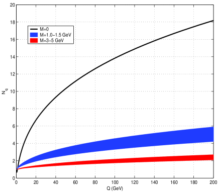
Figure 2: Massless and massive quark jet average multiplicity $N_{Q}$ as a function of the jet hardness $Q$. Bands indicate $m_{c}$ and $m_{b}$ in the $[1,1.5]$ and $[3,5]$ GeV intervals respectively.

5 Heavy quark evolution of second multiplicity correlator

The second multiplicity correlator was first considered for massless quarks in [25]. It is defined in the form $N_{A}^{(2)}=\langle{N_{A}}({N_{A}}-1)\rangle$ in gluon ($A=g$) and quark ($A=q$) jets. The normalized second multiplicity correlator defines the width of the multiplicity distribution and is related to its dispersion squared $D_{A}^{2}=\langle N_{A}^{2}\rangle-N_{A}^{2}$ by the formula (see definitions and notation in section 3)

$$D_{A}^{2}=(F_{A,2}-1)N_{A}^{2}+N_{A}.$$ (41)

The second multiplicity correlators normalized to their own average multiplicity squared are

$$F_{2,g}\equiv G_{2}=\frac{\langle{N_{g}}({N_{g}}-1)\rangle}{N_{g}^{2}},\quad F_{2,q}\equiv Q_{2}=\frac{\langle{N_{q}}({N_{q}}-1)\rangle}{N_{q}^{2}},$$ (42)

inside a gluon and a quark jet respectively. These observables are obtained by integrating the double differential inclusive cross section over the energy fractions $x_{1}=e_{1}/E$ and $x_{2}=e_{2}/E$ of two particles emitted inside the jet,

$$\langle{N_{A}}({N_{A}}-1)\rangle=\iint dx_{1}dx_{2}\left(\frac{1}{\sigma}\frac{d^{2}\sigma}{dx_{1}dx_{2}}\right)_{A}.$$

The system of evolution equations for light quarks following from the MLLA master equation can be written as [5, 18],

$$\frac{d}{dY}(N_{q}^{(2)}-N_{q}^{2})\!\! \!\!=\!\! \!\!\int_{Q_{0}/Q}^{1-Q_{0}/Q}dz\gamma_{0}^{2}(z)P^{(0)}_{qg}(z)N_{g}^{(2)}(Y+\ln z)\!\,,$$ (43)

$$\frac{d}{dY}(N_{g}^{(2)}-N_{g}^{2})\!\! \!\!=\!\! \!\!\int_{Q_{0}/Q}^{1-Q_{0}/Q}dz\gamma_{0}^{2}(z)P^{(0)}_{gg}(z)N_{g}^{(2)}(Y+\ln z)$$ (45)

$$\!\!+\!\! \!\!n_{f}\int_{Q_{0}/Q}^{1-Q_{0}/Q}dz\gamma_{0}^{2}(z)P^{(0)}_{gq}(z)\left[2\Big{(}N_{q}^{(2)}(Y)\!-\!N_{q}^{2}(Y)\Big{)}\!-\!\Big{(}N_{g}^{(2)}(Y)\!-\!N_{g}^{2}(Y)\Big{)}\right.$$ (47)

$$\!\!+\!\! \!\!\left.\Big{(}2N_{q}(Y)-N_{g}(Y)\Big{)}^{2}\right],$$ (49)

with the following relations at DLA [26, 27],

$$N_{q}^{(2)}-N_{q}^{2}=\frac{C_{F}}{N_{c}}\left(N_{g}^{(2)}-N_{g}^{2}\right),\quad N_{q}=\frac{C_{F}}{N_{c}}N_{g}.$$ (50)

The arguments of $N_{A}^{(2)}$ and $N_{A}^{2}$ in the right hand side of the equations do not depend on $z$ because for hard partons $z\sim 1$, the original arguments $Y+\ln z$ and $Y+\ln(1-z)$ of these functions can be approximated to $Y$ after $\ln z$ and $\ln(1-z)$ are neglected. Substituting (16) into (43), after replacing $E\Theta$ by $E(\Theta^{2}+\Theta_{m}^{2})^{1/2}$ in the argument of all logs, taking the bounds (7) and integrating over the regular part of the splitting functions, one has the system

$$\frac{N_{c}}{C_{F}}\frac{d}{d\tilde{Y}}(N_{Q}^{(2)}-N_{Q}^{2})\!\! \!\!=\!\! \!\!\epsilon_{1}(\tilde{Y},L_{m})\int_{\tilde{Y}_{m}}^{\tilde{Y}_{ev}}d\tilde{y}\gamma_{0}^{2}(\tilde{y})N_{g}^{(2)}(\tilde{y})-\epsilon_{2}(\tilde{Y},L_{m})\gamma_{0}^{2}(\tilde{Y})N_{g}^{(2)}(\tilde{Y}),$$ (51)

$$\frac{d}{d\tilde{Y}}(N_{g}^{(2)}-N_{g}^{2})\!\! \!\!=\!\! \!\!\int_{\tilde{Y}_{m}}^{\tilde{Y}_{ev}}d\tilde{y}\gamma_{0}^{2}(\tilde{Y})N_{g}^{(2)}(\tilde{y})-A(\tilde{Y},L_{m})\gamma_{0}^{2}(\tilde{Y})N_{g}^{(2)}(\tilde{Y})$$ (52)

$$\!\!+\!\! \!\!\Big{(}A(\tilde{Y},L_{m})-B(\tilde{Y},L_{m})\Big{)}\gamma_{0}^{2}(\tilde{Y})N_{g}^{2}(\tilde{Y}),$$ (53)

with the initial conditions $N_{A}^{(2)}(L_{m})=\frac{dN_{A}^{(2)}}{d\tilde{Y}}(L_{m})=0$, where

$$B(\tilde{Y},L_{m})=b(n_{f})-\left[2-\frac{n_{f}}{2N_{c}}\left(1-2\frac{C_{F}}{N_{c}}\right)^{2}\right]e^{-\tilde{Y}+L_{m}}+\frac{1}{2}\left[1-\frac{n_{f}}{N_{c}}\left(1-2\frac{C_{F}}{N_{c}}\right)^{2}\right]e^{-2\tilde{Y}+2L_{m}},$$ (54)

with

$$b(n_{f})=\frac{1}{4N_{c}}\left[\frac{11}{3}N_{c}-\frac{2}{3}n_{f}\left(1-2\frac{C_{F}}{N_{c}}\right)^{2}\right].$$

Accordingly, in the massless limit, (51) and (53) reduce to [25, 28]

$$\frac{N_{c}}{C_{F}}\frac{d}{dY}(N_{Q}^{(2)}-N_{Q}^{2})\!\! \!\!=\!\! \!\!\int_{0}^{Y}dy\gamma_{0}^{2}(y)N_{g}^{(2)}(y)-\tilde{\epsilon}_{2}(Y)\gamma_{0}^{2}(Y)N_{g}^{(2)}(Y),$$ (55)

$$\frac{d}{dY}(N_{g}^{(2)}-N_{g}^{2})\!\! \!\!=\!\! \!\!\int_{0}^{Y}dy\gamma_{0}^{2}(y)N_{g}^{(2)}(y)-\tilde{A}(Y)\gamma_{0}^{2}(Y)N_{g}^{(2)}(Y)$$ (56)

$$\!\!+\!\! \!\!\Big{(}\tilde{A}(Y)-\tilde{B}(Y)\Big{)}\gamma_{0}^{2}(Y)N_{g}^{2}(Y),$$ (57)

where

$$\tilde{B}(Y)=b(n_{f})-\left[2-\frac{n_{f}}{2N_{c}}\left(1-2\frac{C_{F}}{N_{c}}\right)^{2}\right]e^{-Y}+{\cal O}\left(e^{-2Y}\right).$$

The functions $\tilde{\epsilon}_{2}(Y)$ and $\tilde{A}(Y)$ are defined above through the equations for the average multiplicity (26) and (27) in light quark jets.

5.1 Approximate solution of the evolution equations

For the gluon jet, taking into account that at high energy scales one has $A\stackrel{{\scriptstyle\tilde{Y}\gg 1}}{{\approx}}A(\tilde{Y},L_{m})$ and $B\stackrel{{\scriptstyle\tilde{Y}\gg 1}}{{\approx}}B(\tilde{Y},L_{m})$ ($\frac{dA,B}{d\tilde{Y}}\stackrel{{\scriptstyle\tilde{Y}\gg 1}}{{\approx}}0$), and making use of (33), the solution reads [29]

$$G_{2}(\tilde{Y},L_{m})-1\stackrel{{\scriptstyle\tilde{Y}\gg 1}}{{\approx}}\frac{1}{3}-C_{1}(\tilde{Y},L_{m})\gamma_{0},$$ (58)

where,

$$C_{1}(\tilde{Y},L_{m})\stackrel{{\scriptstyle\tilde{Y}\gg 1}}{{\approx}}-\frac{2}{9}A(\tilde{Y},L_{m})+\frac{1}{9}\beta_{0}(n_{f})+\frac{2}{3}B(\tilde{Y},L_{m}),\quad\frac{dC_{1}}{d\tilde{Y}}\stackrel{{\scriptstyle\tilde{Y}\gg 1}}{{\approx}}0.$$

Accordingly, for the quark jet one finds [29]

$$Q_{2}(\tilde{Y},L_{m})-1\stackrel{{\scriptstyle\tilde{Y}\gg 1}}{{\approx}}\frac{N_{c}}{C_{F}}\epsilon_{1}^{-1}(\tilde{Y},L_{m})\left(\frac{1}{3}-\tilde{C}_{1}(\tilde{Y},L_{m})\gamma_{0}\right),$$ (59)

where

$$\tilde{C}_{1}(\tilde{Y},L_{m})\stackrel{{\scriptstyle\tilde{Y}\gg 1}}{{\approx}}\frac{5}{18}A(\tilde{Y},L_{m})+\frac{1}{9}\beta_{0}(n_{f})+\frac{1}{6}B(\tilde{Y},L_{m}),\quad\frac{d\tilde{C}_{1}}{d\tilde{Y}}\stackrel{{\scriptstyle\tilde{Y}\gg 1}}{{\approx}}0.$$

Therefore, the correlators $G_{2}$ (58) and $Q_{2}$ (59) are mainly affected by power corrections ${\cal O}(\frac{m}{\tilde{Q}}\sqrt{\alpha_{s}})$ and ${\cal O}(\frac{m^{2}}{\tilde{Q}^{2}}\sqrt{\alpha_{s}})$ which diminish the role of energy conservation in a heavy quark jet and make the correlation stronger as the particle yield gets suppressed inside the dead cone region. Thus, with such effects, the correlators increase as the mass of the leading heavy quark increases and approach the asymptotic DLA values $G_{2}=\frac{4}{3}$ and $Q_{2}=1+\frac{N_{c}}{3C_{F}}$ respectively. However, for realistic energy scales this approximation fails, in particular because of the integration over the dead cone term $\propto\epsilon_{1}(\tilde{Y},L_{m})$ in the double logarithmic contribution of (51). That is why, as we further emphasize in the appendix C, we should rather display the numerical solution of the equations (51) and (53) in the relevant energy range.

6 Phenomenological consequences

The study of multiplicity distributions (mean and higher rank momenta) and inclusive correlations has been traditionally employed in the analysis of multiparticle production in high energy hadron collisions, notably regarding soft (low $p_{t}$) physics (see e.g. [18] and references therein). Moreover, the use of inclusive particle correlations has been recently advocated in the search of new phenomena [30].

On the other hand, it is well known that the study of average charged hadron multiplicities of jets in $e^{+}e^{-}$ collisions has also become a useful tool for testing (perturbative) QCD calculations (see [4, 24] and references therein).

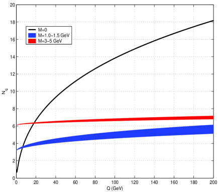
Figure 3: Massless and massive quark jet average multiplicity $N_{Q}^{total}$ as a function of the jet hardness $Q$ including heavy quark flavour decays. Same comments as in Fig. 2.

In this paper we advocate the role of mean multiplicities of jets as a potentially useful signature of new physics when combined with other selection criteria. In Fig. 3, we plot as function of the jet hardness $Q$, the total average jet multiplicity (9), which accounts for the primary state radiation off the heavy quark together with the decay products from the final-state flavoured hadrons, which were introduced in section 3. For these predictions, we set ${\cal K}^{ch}=0.6$ in (9), which we take from [31] and $Q_{0}\sim\Lambda_{QCD}=230$ MeV [5]. Moreover, the flavour decays constants $N_{c}^{dc}=2.60\pm 0.15$ and $N_{b}^{dc}=5.55\pm 0.09$ are independent of the hard process inside the cascade, such that $N_{A}^{dc}$ can be added in the whole energy range. For instance, such values were obtained by the OPAL collaboration at the $Z^{0}$ peak of the $e^{+}e^{-}$ annihilation. In this experiment, $D^{*}$ mesons were properly reconstructed in order to provide samples of events with varying $c$ and $b$ purity. By studying the charged hadron multiplicity in conjunction with samples of varying $b$ purity, it became possible to measure light and heavy quark charged hadron multiplicities separately [14]. As compared to the average multiplicities of the primary state radiation displayed in Fig. 2, after accounting for $N_{A}^{dc}$, the $b$ quark jet multiplicity becomes slightly higher than the $c$ quark jet multiplicity, although both remain suppressed because of the dead cone effect.

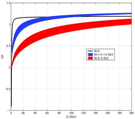
Figure 4: Massless and massive quark jet correlator $Q_{2}$ as a function of the jet hardness $Q$. Same comments as in Fig. 2.

The second quark jet correlator defined in (42) for different flavours is displayed in Fig. 4 as a function of the jet hardness $Q$. Since contributions to the dispersion from quark flavour decays are negligible ($N_{c}^{dc}=2.60\pm 0.15$ and $N_{b}^{dc}=5.55\pm 0.09$) the correlation is the strongest for partons at the primary state radiation of the process. Notice that, while the $u,d,s$ and the $c$ quark correlators are of the same order of magnitude for a jet hardness $Q\gtrsim 40$ GeV as relevant energy range, the vertical difference with the $b$ quark correlator, which is weaker, can still exceed $\sim 20\%$. Therefore, the measurement of the quark correlator should provide a further signature of $b$ flavour and associated exotic particles yield when compared with $u,d,s,c$ correlators. Finally, the variation of the charged hadrons average multiplicities and the correlator in the above-mentioned intervals for the charm and and bottom masses turns out to be negligible for our purposes.

7 Conclusions

Jet physics has been so far of paramount importance in the rise and development of the SM and expectedly will keep such a prominent role in the discovery of new phenomena at hadron colliders like the Tevatron and the LHC. However, QCD jets represent a formidable challenge to disentangle signals of new physics from hadronic background in most cases. On the other hand, plenty of new physics channels end with heavy flavours in the final state, before fragmenting and hadronizing.

Thus, our present work focusing on the differences of the average charged hadron multiplicity between jets initiated by gluons, light or heavy quarks could indeed represent a helpful auxiliary criterion to tag such heavy flavours from background for jet hardness $Q\gtrsim 40$ GeV. Notice that we are suggesting as a potential signature the a posteriori comparison between average jet multiplicities corresponding to different samples of events where other criteria to discriminate heavy from light quark initiated jets were first applied. In other words, one should compare mean multiplicities at different jet-hardness $Q$, in order to check that they agree with QCD predictions. Fig.3 plainly demonstrate that the separation between light quark jets and heavy quark jets is allowed above a few tens of GeV with the foreseen errors of the experimentally measured average multiplicities of jets. The difference between light quark jet multiplicities and heavy quark jet multiplicities $N_{q}-N_{Q}$ in one jet is exponentially increasing because of suppression of forward gluons in the angular region around the heavy quark direction. This result is not drastically affected after accounting for heavy flavour decays multiplicities, such that it can still be used as an important signature for the search of new physics in a jet together with other selection criteria. However, our result can only be applied to single jets and therefore, it should not be extrapolated to the phenomenology of the $Q\bar{Q}$ dipole treated in [4] because neither interference effects with other jets nor large angle gluon emissions are considered in our case. As a complementary observable, in particular for $b$-tagging, the second multiplicity correlator (42) displayed in Fig. 4 should also contribute to discriminate $b$ quark from $u,d,s,c$ quark channels. Indeed, while the $c$ quark correlator remains of the same order of magnitude than the light quark jet correlator, the $b$ quark correlator gets weaker by 20$\%$ and therefore, distinguishable with respect to the other quarks in the relevant energy range. Furthermore, the inclusion of the heavy quark mass in the evolution equations for the correlator does not affect the asymptotic energy independent flattening of the slope arising from the KNO (Koba-Nielsen-Olsen) scaling [32].

Notice that the measurement of such observables require the previous reconstruction of jets at hadron colliders. Thanks to important recent developments on jet reconstruction algorithms [33, 35, 34], future analysis such as single inclusive hadron production inside light and heavy quark jets look very promising.

Appendix A From AO to the incoherence condition of gluon emission off the heavy quark

In the MLLA, the parton decay probabilities are written in a form [5],

$$d^{2}_{Qg}\equiv d^{2}\sigma_{Q\to Qg}=\frac{\alpha_{s}}{2\pi}P^{(0)}_{Qg}(z)dzV(\vec{n})\frac{d\Omega}{8\pi},\quad V_{g(Q)}^{g^{\prime}}(\vec{n})=\frac{a_{g^{\prime}Q}+a_{gQ}-a_{g^{\prime}gf}}{a_{g^{\prime}g}a_{g^{\prime}Q}}.$$ (60)

Figure 5: Second gluon emission off the primary gluon in the process $Q\to\bar{Q}+g(f)+g^{\prime}(s)$.

It describes the process $Q\to\bar{Q}+g(f)+g^{\prime}(s)$ displayed in Fig.5, where the subscripts mean father and son. In this case we define $\Theta=\Theta_{gQ}$, $\Theta^{\prime}=\Theta_{g^{\prime}g}$. For light quarks involved in the same process $q\to\bar{q}+g(f)+g^{\prime}(s)$, if “i” and “k” denote the massless particles, then the angular factor $a_{ik}$ in the relativistic case is written as

$$a_{ik}=1-\cos\Theta_{ik}.$$ (61)

After taking the azimuthal average around the “son” gluon direction, one obtains [5],

$$\left<V_{g(q)}^{g^{\prime}}\right>=\int_{0}^{2\pi}\frac{d\phi}{2\pi}V_{g(q)}^{g^{\prime}}(\vec{n})=\frac{2}{a_{g^{\prime}g}}\vartheta(a_{gq}-a_{g^{\prime}g}),$$ (62)

with $\vartheta$ the Heaviside function. This leads to the exact AO inside partonic cascades by replacing the strong AO in the DLA $\Theta^{\prime}\ll\Theta$ by $\Theta^{\prime}\leq\Theta$ in the MLLA. For massive particles we may write (60) in the same form after replacing the standard massless splitting functions [5] by the massive one [10]. If the leading parton is a heavy quark, the angular factor of the emitted gluon $``g"$ off the heavy quark $Q$, can be checked after some simple kinematics, to be written in the form,

$$a_{gQ}=1-\sqrt{1-\Theta_{m}^{2}}\cos\Theta,$$ (63)

where $\Theta_{m}$ is the angle of the dead cone. In this case, (62) can be rewritten as follows

$$\left<V_{g(Q)}^{g^{\prime}}\right>=\int_{0}^{2\pi}\frac{d\phi}{2\pi}V_{g(Q)}^{s}(\vec{n})=\frac{2}{a_{g^{\prime}g}}\vartheta(a_{gQ}-a_{g^{\prime}g}),$$ (64)

imposing that $\cos\Theta^{\prime}\geq\sqrt{1-\Theta_{m}^{2}}\cos\Theta$. For small angles, if one sets $\cos\Theta\approx 1-\frac{\Theta^{2}}{2}$ in both members of the previous inequality, one gets the incoherent condition:

$$\Theta^{\prime 2}\leq\Theta^{2}+\Theta_{m}^{2}.$$ (65)

In the massless case $\Theta_{m}=0$, (65) simply reduces to the standard exact AO $\Theta^{\prime}\leq\Theta$.

Appendix B Accompanying radiated quanta off the heavy quark dipole

In [4, 13], the probability of soft gluon emission of the heavy quark pair $Q\bar{Q}$ produced in the $e^{+}e^{-}$ annihilation was written in the form,

$$d^{2}\sigma_{Q\bar{Q}g}=\frac{C_{F}\alpha_{s}(\kappa_{\perp}^{2})}{\pi}\frac{dz}{z}\frac{\beta}{v}d\cos\Theta_{c}\left\{2(1-z)\frac{\beta^{2}\sin^{2}\Theta_{c}}{(1-\beta^{2}\cos^{2}\Theta_{c})^{2}}+z^{2}\left[\frac{1}{1-\beta^{2}\cos^{2}\Theta_{c}}-\frac{1}{2}\right]\zeta_{V}^{-1}\right\},$$ (66)

where $z$ is the energy fraction of the emitted gluon and $\Theta_{c}$ the emission angle with respect to the center of mass of the $Q\bar{Q}$ pair. Moreover, the following notation was introduced:

$$\beta^{2}=1-\frac{4m^{2}}{W^{2}(1-z)},\quad v^{2}=1-\frac{4m^{2}}{W^{2}},\quad\zeta_{V}=1+2\frac{m^{2}}{W^{2}}.$$ (67)

The transverse momentum of the gluon appearing on the argument of the running coupling in (66) was written in the form,

$$\kappa_{\perp}^{2}=\left(\frac{zW}{2}\right)^{2}(1-\beta^{2}\cos^{2}\Theta_{c})^{2}.$$ (68)

With such a notation, we now take interest in the soft ($1-z\sim 1$) and collinear ($\Theta_{c}\ll 1$) limits of (66) and set $W\to 2E$ in order to reduce (66) to the single jet event initiated by a heavy quark $Q$. Thus, the terms take the following form

• $$\beta^{2}\stackrel{{\scriptstyle z\ll 1}}{{\approx}}1-\frac{m^{2}}{E^{2}}=1-\Theta_{m}^{2},\quad(1-\beta^{2}\cos^{2}\Theta_{c})^{2}\stackrel{{\scriptstyle z\ll 1,\Theta_{c}\ll 1}}{{\approx}}(\Theta_{c}^{2}+\Theta_{m}^{2})^{2},$$

• $$\frac{2(1-z)\beta^{2}\sin^{2}\Theta_{c}}{(1-\beta^{2}\cos^{2}\Theta_{c})^{2}}\stackrel{{\scriptstyle z\ll 1,\Theta_{c}\ll 1}}{{\approx}}\frac{2(1-z)\Theta_{c}^{2}}{(\Theta_{c}^{2}+\Theta_{m}^{2})^{2}},\;\;\left[\frac{z^{2}}{1-\beta^{2}\cos^{2}\Theta_{c}}-\frac{1}{2}\right]\zeta_{V}^{-1}\stackrel{{\scriptstyle z\ll 1,\Theta_{c}\ll 1}}{{\approx}}\frac{z^{2}}{\Theta_{c}^{2}+\Theta_{m}^{2}}.$$

The term proportional to $-\frac{1}{2}$ in the cross section (66) does contribute neither as a soft logarithmic contribution nor as a collinear one, and therefore can be neglected in this approximation. It should correspond to a Feynman diagram which only accounts for interference effects between the $Q$ and the $\bar{Q}$ jets in the $Q\bar{Q}$ antenna. In this limit, for one jet we set $d^{2}\sigma_{Q\bar{Q}g}\to d^{2}\sigma_{Qg}$, $\Theta_{c}\to\Theta$ and $\frac{\beta}{v}\to 1$, such that the dipole cross section (66) can be rewritten in the form

$$d^{2}\sigma_{Qg} \simeq \frac{C_{F}}{N_{c}}\gamma_{0}^{2}(\kappa_{\perp}^{2})\frac{d\Theta^{2}}{\Theta^{2}+\Theta_{m}^{2}}\left\{\frac{1}{z}\frac{\Theta^{2}}{\Theta^{2}+\Theta_{m}^{2}}-1+\frac{z}{2}+\frac{\Theta_{m}^{2}}{\Theta^{2}+\Theta_{m}^{2}}\right\}dz$$

$$\equiv \gamma_{0}^{2}(\kappa_{\perp}^{2})\frac{d\kappa_{\perp}^{2}}{\kappa_{\perp}^{2}}P^{(0)}_{Qg}(z)dz,$$

as given in (15), where $P^{(0)}_{Qg}(z)$ was written in (16), while (68) was reduced to the following,

$$\kappa_{\perp}^{2}\stackrel{{\scriptstyle z\ll 1,\Theta_{c}\ll 1}}{{\approx}}z^{2}E^{2}(\Theta^{2}+\Theta_{m}^{2})\equiv z^{2}\tilde{Q}^{2},\quad\tilde{Q}^{2}=E^{2}(\Theta^{2}+\Theta_{m}^{2}).$$

Therefore, in the soft and collinear approximation, the dipole case (66) reduces to the jet event (B), which coincides with the expression given in (15). In the massless case $\Theta_{m}=0$, it simplifies to the standard DGLAP kernel as explained in [4],

$$d^{2}\sigma_{Qg}\propto\frac{d\Theta^{2}}{\Theta^{2}}\left\{2(1-z)+z^{2}\right\}\frac{dz}{z}.$$

Appendix C Analytical versus numerical solution of the heavy quark correlator equation (51)

In Fig. 6 we display the analytical solution together with the numerical solution of (51) for the second multiplicity correlator $Q_{2}$ defined in (42). As it can be seen, when the mass of the leading heavy quark increases, the approximated analytical correlator becomes slightly stronger. However, because of forward gluon suppression taken into account by the integrated function $\epsilon_{1}(\tilde{Y},L_{m})$ in the leading DL contribution of (51), such a behaviour cannot be trusted for lower virtualities than few thousands of GeV. That is why, even if the shape of the analytical solution may be correct for $Q\gtrsim 100$ GeV, we should only trust the shape and normalization of the numerical solution in a much wider energy range $Q\gtrsim 40$ GeV in view of realistic QCD predictions.

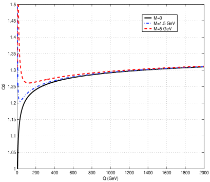
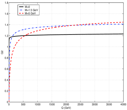
Figure 6: Analytical (left) versus numerical (right) solution of equation (51) for the second multiplicity correlator $Q_{2}$ defined in (42).

References

- [1] E. Leader and E. Predazzi. An Introduction to gauge theories and modern particle physics. Vol. 2: CP violation, QCD and hard processes. Camb. Monogr. Part. Phys. Nucl. Phys. Cosmol., 4:1–431, 1996.
- [2] G. Aad et al. Expected Performance of the ATLAS Experiment - Detector, Trigger and Physics. 2009.
- [3] Yuri L. Dokshitzer, Valery A. Khoze, and S. I. Troian. On specific QCD properties of heavy quark fragmentation (’dead cone’). J. Phys., G17:1602–1604, 1991.
- [4] Yuri L. Dokshitzer, Fabrizio Fabbri, Valery A. Khoze, and Wolfgang Ochs. Multiplicity difference between heavy and light quark jets revisited. Eur. Phys. J., C45:387–400, 2006.
- [5] Yuri L. Dokshitzer, Valery A. Khoze, Alfred H. Mueller, and S. I. Troian. Gif-sur-Yvette, France: Ed. Frontieres (1991) 274 p. (Basics of).
- [6] G. Curci, W. Furmanski, and R. Petronzio. Evolution of Parton Densities Beyond Leading Order: The Nonsinglet Case. Nucl. Phys., B175:27, 1980.
- [7] W. Furmanski and R. Petronzio. Lepton - Hadron Processes Beyond Leading Order in Quantum Chromodynamics. Zeit. Phys., C11:293, 1982.
- [8] John C. Collins. Hard-scattering factorization with heavy quarks: A general treatment. Phys. Rev., D58:094002, 1998.
- [9] V. N. Baier, Victor S. Fadin, and Valery A. Khoze. Quasireal electron method in high-energy quantum electrodynamics. Nucl. Phys., B65:381–396, 1973.
- [10] Frank Krauss and German Rodrigo. Resummed jet rates for e+ e- annihilation into massive quarks. Phys. Lett., B576:135–142, 2003.
- [11] Stefan Kluth. Tests of quantum chromo dynamics at e+ e- colliders. Rept. Prog. Phys., 69:1771–1846, 2006.
- [12] Yakov I. Azimov, Yuri L. Dokshitzer, Valery A. Khoze, and S. I. Troyan. Similarity of Parton and Hadron Spectra in QCD Jets. Z. Phys., C27:65–72, 1985.
- [13] Yuri L. Dokshitzer, Valery A. Khoze, and S. I. Troian. Specific features of heavy quark production. LPHD approach to heavy particle spectra. Phys. Rev., D53:89–119, 1996.
- [14] R. Akers et al. A Measurement of charged particle multiplicity in Z0 c anti-c and Z0 b anti-b events. Phys. Lett., B352:176–186, 1995.
- [15] Combined preliminary data on parameters from the LEP experiments and constraints on the Standard Model. Contributed to the 27th International Conference on High- Energy Physics - ICHEP 94, Glasgow, Scotland, UK, 20 - 27 Jul 1994.
- [16] R. Keith Ellis, W. James Stirling, and B. R. Webber. QCD and collider physics. Camb. Monogr. Part. Phys. Nucl. Phys. Cosmol., 8:1–435, 1996.
- [17] Michael Edward Peskin and Daniel V. Schroeder. An Introduction to quantum field theory. Reading, USA: Addison-Wesley (1995) 842 p.
- [18] I. M. Dremin and J. W. Gary. Hadron multiplicities. Phys. Rept., 349:301–393, 2001.
- [19] F. E. Low. Bremsstrahlung of very low-energy quanta in elementary particle collisions. Phys. Rev., 110:974–977, 1958.
- [20] T. H. Burnett and Norman M. Kroll. Extension of the low soft photon theorem. Phys. Rev. Lett., 20:86, 1968.
- [21] A. Capella, I. M. Dremin, J. W. Gary, V. A. Nechitailo, and J. Tran Thanh Van. Evolution of average multiplicities of quark and gluon jets. Phys. Rev., D61:074009, 2000.
- [22] Alfred H. Mueller and P. Nason. HEAVY PARTICLE CONTENT IN QCD JETS. Nucl. Phys., B266:265, 1986.
- [23] Vincent Mathieu, Nikolai Kochelev, and Vicente Vento. The Physics of Glueballs. Int. J. Mod. Phys., E18:1–49, 2009.
- [24] A. V. Kisselev and V. A. Petrov. Multiple hadron production in e+e- annihilation induced by heavy primary quarks. New analysis. Phys. Part. Nucl., 39:798–809, 2008.
- [25] E. D. Malaza and B. R. Webber. MULTIPLICITY DISTRIBUTIONS IN QUARK AND GLUON JETS. Nucl. Phys., B267:702, 1986.
- [26] Yuri L. Dokshitzer, Victor S. Fadin, and Valery A. Khoze. Double Logs of Perturbative QCD for Parton Jets and Soft Hadron Spectra. Zeit. Phys., C15:325, 1982.
- [27] Yuri L. Dokshitzer, Victor S. Fadin, and Valery A. Khoze. On the Sensitivity of the Inclusive Distributions in Parton Jets to the Coherence Effects in QCD Gluon Cascades. Z. Phys., C18:37, 1983.
- [28] I. M. Dremin, C. S. Lam, and V. A. Nechitailo. High order perturbative QCD approach to multiplicity distributions of quark and gluon jets. Phys. Rev., D61:074020, 2000.
- [29] Redamy Perez Ramos. Medium-modified evolution of multiparticle production in jets in heavy-ion collisions. J. Phys., G36:105006, 2008.
- [30] Miguel-Angel Sanchis-Lozano. Prospects of searching for (un) particles from Hidden Sectors using rapidity correlations in multiparticle production at the LHC. Int. J. Mod. Phys., A24:4529–4572, 2009.
- [31] T. Aaltonen et al. Two-Particle Momentum Correlations in Jets Produced in Collisions at = 1.96-TeV. Phys. Rev., D77:092001, 2008.
- [32] Z. Koba, Holger Bech Nielsen, and P. Olesen. Scaling of multiplicity distributions in high-energy hadron collisions. Nucl. Phys., B40:317–334, 1972.
- [33] Matteo Cacciari and Gavin P. Salam. Dispelling the N**3 myth for the k(t) jet-finder. Phys. Lett., B641:57–61, 2006.
- [34] Matteo Cacciari and Gavin P. Salam. Pileup subtraction using jet areas. Phys. Lett., B659:119–126, 2008.
- [35] Matteo Cacciari, Gavin P. Salam, and Gregory Soyez. The Catchment Area of Jets. JHEP, 04:005, 2008.