Quantum phase transitions Quantized spin models, including quantum spin frustration Quantum error correction and other methods for protection against decoherence

Compass-Heisenberg model on the square lattice
— spin order and elementary excitations

Abstract

We explore the physics of the anisotropic compass model under the influence of perturbing Heisenberg interactions and present the phase diagram with multiple quantum phase transitions. The macroscopic ground state degeneracy of the compass model is lifted in the thermodynamic limit already by infinitesimal Heisenberg coupling, which selects different ground states with $\mathbb{Z}_{2}$ symmetry depending on the sign and size of the coupling constants — then low energy excitations are spin waves, while the compass states reflecting columnar order are separated from them by a macroscopic gap. Nevertheless, nanoscale structures relevant for quantum computation purposes may be tuned such that the compass states are the lowest energy excitations, thereby avoiding decoherence, if a size criterion derived by us is fulfilled.
Published in: EPL 91, 40005 (2010).

Strongly correlated electrons in transition metal oxides lead to rich quantum physics controlled by spin and orbital superexchange interactions that are complex and often intrinsically frustrated due to competing interactions [1, 2]. A high frustratedness is realized in the orbital compass model [3, 4, 5, 6, 7], resulting in a large degeneracy of ground states. In contrast to SU(2) Heisenberg interactions which are not frustrated and isotropic in spin space, compass interactions are locally Ising-like but the spin component involved in the interactions depends on the bond orientation. Recent interest in the compass model was triggered by the observations that it has an interdisciplinary character and plays an important role in a variety of contexts. It could: ($i$) serve as an effective model for protected qubits realized by Josephson arrays [6], or ($ii$) describe polar molecules in optical lattices and systems of trapped ions [8]. First experimental successes in constructing special networks of Josephson junctions guided by the compass model have already been reported [9].

Materials with large spin-orbit coupling may give rise to compass spin interactions for some lattice structures [10], leading either to the compass or the Kitaev honeycomb model [11]. Numerical studies [12, 13] and the mean-field approach [14] suggest that when anisotropic interactions are varied through the isotropic point of the two-dimensional (2D) compass model, a quantum phase transition (QPT) between two different types of directional order occurs. Recently the existence of this transition, similar to the one found in the exact solution of the one-dimensional (1D) compass model [15], was confirmed using projected entangled-pair state algorithm [16]. This implies that the symmetry is spontaneously broken at the compass point, and the spin orientation follows one of two equivalent interactions, as concluded recently within the multiscale entanglement renormalization ansatz (MERA) [17].

In this Letter we introduce a generalized 2D Compass-Heisenberg (CH) model and investigate to what extent the degenerate ground states of the quantum compass model are robust with respect to perturbing interactions which may occur due to an imperfect design of the system. General perturbations could therefore prohibit the conservation of non-local quantities characteristic of the compass model [12, 6, 19]. We assume that such interactions are of Heisenberg type, as suggested by possible solid state applications [10, 18]. We have found that the compass ground state is fragile and an infinitesimal Heisenberg coupling is sufficient to lift its semi-macroscopic (exponential in linear size) degeneracy and to generate magnetic long range order, either ferromagnetic (FM) or antiferromagnetic (AF) one, which privileges a pair of columnar compass states as the ground state, while the other compass states survive as finite energy excitations. Indeed, the phase diagram of the CH model, shown in Fig. 1, appears to be very rich and exhibits different QPTs between various phases of $\mathbb{Z}_{2}$ symmetry [20] triggered via softening either of spin waves or of a semi-macroscopic number of quantum states.

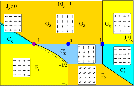
Figure 1: Phase diagram of the CH model Eq. (1) with AF compass coupling $J_{z}>1$. Square and diamond mark the isotropic compass points $J_{x}=\pm J_{z}$, where in each case four ordered phases meet. For a phase $\Phi_{\alpha}=G_{z},C^{\prime}_{z},F_{x},\cdots$, $\Phi$ denotes the spin order depicted in the corresponding inset (i.e., $F$ for a FM phase, $G$ or $C$ for AF phases) and $\alpha=x,y,z$ the spin orientation. The QPT between $F_{x}$ and $C^{\prime}_{z}$ phases (solid line) is affected by quantum corrections to the classical transition (dashed line), see text.

We consider a CH model of spins $1/2$ on the square lattice

$${\cal H} = \sum_{i,j}\left(J_{x}\sigma^{x}_{i,j}\sigma^{x}_{i,j+1}+J_{z}\sigma^{z}_{i,j}\sigma^{z}_{i+1,j}\right)$$ (1)

$$+ I\sum_{i,j}\big{(}\vec{\sigma}_{i,j}\cdot\vec{\sigma}_{i,j+1}+\vec{\sigma}_{i,j}\cdot\vec{\sigma}_{i+1,j}\big{)}\,,$$

with $\{\sigma^{\alpha}_{i,j}\}$ being Pauli matrices, $\vec{\sigma}_{i,j}=\{\sigma^{x}_{i,j},\sigma^{y}_{i,j},\sigma^{z}_{i,j}\}$, and two types of nearest neighbour interactions along bonds in the 2D lattice: ($i$) the frustrated compass interactions $\{J_{x},J_{z}\}$ which couple $\{\sigma^{\alpha}_{i,j}\}$ components along $\alpha$-oriented bonds (the two axes are labelled $\alpha=x,z$), and ($ii$) Heisenberg interactions of amplitude $I$. We will use hereafter $\phi$ and $J_{c}$ to define interaction parameters such that

$$J_{z}\equiv J_{c}\cos\phi\,,\hskip 28.45274ptJ_{x}\equiv J_{c}\sin\phi\,,$$ (2)

with $J_{c}\equiv 1$ serving as a unit. Numerical results are obtained with Lanczos exact diagonalizations for periodic 2D rectangular clusters with even number of sites of up to $N=36$ ($N=L_{x}\times L_{z}$ with $L_{x}$ and $L_{z}$ longitudinal dimensions, except for $N=18$ and $N=32$ clusters which are rotated, see Ref. [21]). Lattice symmetries (translations and $C_{2v}$ point group) and the $\sigma^{z}_{\bf{r}}\rightarrow-\sigma^{z}_{\bf r}$ symmetry (for any ${\bf r}=(i,j)$) are used to reduce the size of the Hilbert space; note that in contrast to the Heisenberg model $\sigma^{z}_{\rm tot}=\sum_{i}\sigma^{z}_{\bf r}$ is not conserved, but only the parity $P=(-1)^{\sigma^{z}_{\rm tot}/2}$.

We first examine the effect of Heisenberg interactions $I>0$ favouring $G_{z}$-type (Néel) AF order (Fig. 1). For AF anisotropic compass couplings $J_{z}>|J_{x}|$ spins orient along the $z$ axis and form AF columnar states that are subsequently linked by positive $I$ into the $G_{z}$-AF structure. The spin structure factor

$$S^{z}_{\bf k}\equiv\frac{1}{N}\sum_{\bf r}e^{i\bf{k}\cdot\bf{r}}\langle\sigma_{\bf 0}^{z}\sigma_{\bf r}^{z}\rangle$$ (3)

(normalized so that $S^{z}_{\bf{k}}=\delta_{\bf{k},\bf{Q}}$ with $\bf{Q}=(\pi,\pi)$ for a Néel state) probes the onset of 2D spin order expected for increasing $I/J_{c}$, see Fig. 2(a). The compass regime with columns uncorrelated between one another, indicated by $S^{z}_{\bf{k}}$ being maximal at $k_{z}=\pi$ and independent of $k_{x}$ [22], changes surprisingly fast into the $G_{z}$-AF order — the expected peak at $\bf{k}=\bf{Q}$ grows rapidly with increasing $I/J_{c}$ and is already of the order of unity for $I/J_{c}\simeq 0.01$ ! In contrast, the peaks at $\bf{k}=\bf{Q}$ in spin structure factors $S^{y}_{\bf{k}}$ [see Fig. 2(b)] and $S^{x}_{\bf{k}}$ (not shown) grow slowly with $I/J_{c}$ and are much smaller than $S^{z}_{\bf Q}$ in the range of $0<I/J_{c}<1$, which reflects the spin anisotropy and $\mathbb{Z}_{2}$ symmetry of the ordered $G_{z}$ phase; eventually this anisotropy weakens for increasing $I/J_{c}$.

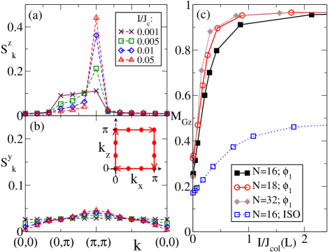
Figure 2: Spin structure factors (a) $S^{z}_{\bf{k}}$, and (b) $S^{y}_{\bf{k}}$, for the $N=36$-site periodic cluster ($L_{x}=L_{z}=6$) with isotropic AF compass couplings ($J_{x}=J_{z}$) for selected ${\bf k}=(k_{x},k_{z})$, see inset in (b), and different $I/J_{c}$. (c): Order parameter $M_{Gz}$ for cluster sizes $N=16,18,32$ for increasing $I/J_{\rm col}(L)$ (5). Solid (dotted) lines for an anisotropy parameter $\phi_{1}=\tan^{-1}(J_{x}/J_{z})=3\pi/20$ and the isotropic compass model (ISO) $\phi=\pi/4$.

The onset of the $G_{z}$-AF phase for $I\ll J_{c}$ can be understood using perturbation theory for small both $J_{x}/J_{z}$ and $I/J_{z}$. The unperturbed Hamiltonian (1D $J_{z}$ couplings) selects a manifold of $2^{L_{x}}$ column-ordered ground states, each column $j=1,\cdots,L_{x}$ possessing a $S=1/2$ degree of freedom is represented here by $\tau_{j}^{z}=\pm 1$, depending on the orientation of a reference spin in the column.

In L’th order two neighbouring columns are flipped via the horizontal compass couplings

$$H_{\rm col}=J_{\rm col}(L)\sum_{j}\tau_{j}^{x}\tau_{j+1}^{x}\,,$$ (4)

with a coupling constant

$$J_{\rm col}(L)=8J_{z}c_{L}(J_{x}/8J_{z})^{L}\,,$$ (5)

which gets exponentially small with increasing column length $L\equiv L_{z}$ for finite systems considered here. Here $c_{L}$ is a constant increasing with $L$ ($c_{L}=20$, 252, 3432 for $L=4$, 6, 8 [12]). $J_{\rm col}(L)$ vanishes in the thermodynamic limit for $J_{x}/J_{z}\leq 1$, explaining the (at least $2^{L_{x}}$-fold) ground state degeneracy of the compass model. In contrast, Heisenberg interactions couple the $\{\sigma^{z}_{i,j},\sigma^{z}_{i,j+1}\}$ components in neighbouring columns, and this results in a first order perturbative coupling $L_{z}I\tau_{j}^{z}\tau_{j+1}^{z}$ which favours an AF arrangement between the columns $j$ and $(j+1)$. This second term obviously dominates the first one ($J_{\rm col}$) in the thermodynamic limit as soon as $I\neq 0$, which thus ensures the onset of the $G_{z}$-AF long range order. This is indeed confirmed by the evolution of the order parameter $M_{Gz}\equiv S^{z}_{(\pi,\pi)}$ as a function of $I/J_{\rm col}$ shown in Fig. 2(c) — while $J_{\rm col}$ varies over several orders of magnitude between clusters considered, the values of $M_{Gz}$ are almost identical for a given ratio $J_{x}/J_{z}$.

The isotropic ($J_{x}=J_{z}$) case is specific, as $S^{z}_{\bf Q}$ saturates then close to $\frac{1}{2}$ (rather than close to 1) for $J_{\rm col}\ll I<J_{c}$, and so does $S^{x}_{\bf Q}$. In this case the compass interactions favour a manifold of $(2^{L_{x}}+2^{L_{z}})$-degenerate ground states (in the thermodynamic limit), among which row-ordered states with spins along $x$ (along with column-ordered states considered above); the perturbing Heisenberg interactions select in this manifold the four Néel states with ordered spin components either $\sigma^{z}_{\bf r}$ ($G_{z}$ phase favoured for $J_{z}\geq J_{x}$) or $\sigma^{x}_{\bf r}$ ($G_{x}$ phase for $J_{x}\geq J_{z})$. This symmetry breaking was recently studied in the compass model (at $I=0$) using the MERA [17].

The perturbative treatment allows us to identify various ordered phases which develop from the $I=0$ line in the phase diagram of Fig. 1. For instance, the $C^{\prime}_{z}$ phase (with order parameter $M_{C}\equiv S^{z}_{(0,\pi)}$) is found when the dominant compass coupling $J_{z}>0$ favours AF-ordered columns while a small $I<0$ couples neighbouring columns ferromagnetically. Thus, the compass model ($I=0$ line) is at a transition between two phases, and four different phases meet at the isotropic points $J_{x}=\pm J_{z}$ (square and diamond in Fig. 1), showing that both QPTs in the compass model evolve into transition lines between phases with different types of spin order.

Investigating the phase diagram of the CH model (Fig. 1), perturbative approaches cannot be applied when Heisenberg interactions are comparable to dominant compass terms, especially when they frustrate each other, e.g. for $|J_{x}|\leq J_{z}$, $I<0$ and $|I/J_{z}|=O(1)$. For large negative Heisenberg couplings FM phases are favoured — with spins being perpendicular to the $z$ axis to avoid AF compass couplings. Depending on the sign of $J_{x}$, the most favourable spin orientation is either along $x$ ($F_{x}$ phase with order parameter $M_{Fx}\equiv S^{x}_{(0,0)}$ for $J_{x}<0$) or along $y$ ($F_{y}$ phase with $M_{Fy}\equiv S^{y}_{(0,0)}$ for $J_{x}>0$), not found within the compass ground states manifold. By comparing the classical energies (per site) of different phases, we determined the classical transition lines in Fig. 1. For instance, the phase transitions between the $C^{\prime}_{z}$ phase and both above FM phases ($F_{x}$ and $F_{y}$), were found using: $E_{0}(C^{\prime}_{z})=-J_{z}$, $E_{0}(F_{x})=J_{x}+2I$, and $E_{0}(F_{y})=2I$.

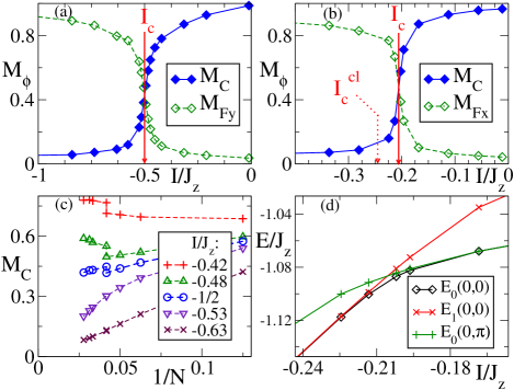
Figure 3: Order parameters $M_{\phi}$ of the $C^{\prime}_{z}$ phase ($M_{C}$), and (a) of the $F_{y}$ phase with $\phi=\pi/10$; (b) of the $F_{x}$ phase with $\phi=37\pi/20$. $I_{c}$ indicates the transition between $C^{\prime}_{z}$ and either (a) $F_{y}$ phase, or (b) $F_{x}$ phase — in (b) its classical counterpart $I_{c}^{\rm cl}$ is also shown. (c): Size-dependence of $M_{C}$ for values $I/J_{x}$ close to the transition displayed in (a). (d): Momentum-resolved lowest energy levels per site ($E_{n}(\bf{k})$ is the $(n+1)^{th}$ state of momentum $\bf{k}$) on a $N=32$-site cluster, across the transition displayed in (b). The ground state energy $E_{0}(0,0)$ shows avoiding crossing.

Strikingly, the phase diagram of the quantum model (Fig. 1) differs very little from that found by comparing classical energies. First, some transition lines are not modified by quantum fluctuations. This occurs due to additional symmetries at the classical transition line. An example is the case of $J_{x}=J_{z}>0$ and $I>0$ discussed previously, where the Hamiltonian is invariant under a $\pi/2$ rotation of both spins and lattice along the $y$ axis. The first order transition point between two symmetry-broken compass phases, found at $J_{z}=J_{x}$ in the compass model [16] (square in Fig. 1), extends to a more conventional (still first order) transition line between the fully (classically) ordered $G_{z}$ and $G_{x}$ phases, stable for either $J_{z}>J_{x}$ or $J_{z}<J_{x}$.

Similarly, on the line defined by $I=-J_{z}/2$ and $0<J_{x}<J_{z}$ (classical transition line between $C^{\prime}_{z}$ and $F_{y}$ phases), the Hamiltonian Eq. (1) has an additional U(1) symmetry [23], and therefore the corresponding QPT occurs necessarily along this line. We have checked by considering bond correlations $\langle\sigma_{\bf 0}^{\alpha}\sigma_{\bf r}^{\beta}\rangle$ for $\alpha\neq\beta$ that no other intermediate (e.g. spiral) ordered phase develops in this range of parameters. For both phases, the dependences of order parameters on $I/J_{z}$ and on cluster size [shown for fixed $\phi=\pi/10$ in Fig. 3(a), with size-scalings of $M_{C}$ in Fig. 3(c)] indicate a first order transition by the slope of order parameter which increases with $N$ at the transition, see Fig. 3(a). The scaling with increasing size indicates a discontinuity across the $I=-J_{z}/2$ point, whereas both order parameters are equal at this point and extrapolate to a finite value in the thermodynamic limit.

We emphasize that, contrary to what happens usually in first order transitions, no level crossing occurs in the ground state for finite clusters (see also Refs. [16] and [24]), where the preferred spin orientation evolves continuously from the $z$ axis (in the $C^{\prime}_{z}$ phase) to the $y$ axis ($F_{y}$), but a level crossing occurs between the two lowest excitations, as shown for the $C^{\prime}_{z}-F_{x}$ transition in Fig. 3(d). This is related to the distinct broken symmetries in both phases in the thermodynamic limit: ($i$) translation symmetry breaking along $z$ in the $C^{\prime}_{z}$ phase results in a 2-fold degenerate ground state with ${\bf k}=(0,0)$ and $(0,\pi)$ momenta, while ($ii$) the spontaneous breaking of $\mathbb{Z}_{2}$ symmetry in the $F_{y}$ (or $F_{x}$) phase results in a 2-fold ground state degeneracy, both states with ${\bf k}=(0,0)$ momentum [but with different parity $P=(-1)^{\sigma^{z}_{\rm tot}/2}$]. The crossing between the second $(0,0)$ and the lowest $(0,\pi)$ states occurs exactly at $I=-J_{z}/2$ in the $C^{\prime}_{z}-F_{y}$ transition, for the above symmetry reasons.

In contrast, some QPTs in the phase diagram of Fig. 1, e.g. the $C^{\prime}_{z}-F_{x}$ transition (dashed line), do not present additional symmetries at the classical level and are affected by quantum fluctuations. The energies (per site) of $C^{\prime}_{z}$ and $F_{x}$ phase, evaluated in second order perturbation theory, are:

$$E(C^{\prime}_{z}) = E_{0}(C^{\prime}_{z})-\frac{J_{x}^{2}}{8J_{z}+4I}-\frac{I^{2}}{J_{z}-I}\,,$$ (6)

$$E(F_{x}) = E_{0}(F_{x})+\frac{J_{z}^{2}}{8J_{x}+12I}\,.$$ (7)

They are equal on the solid line separating both phases in Fig. 1. Note that numerical estimations of the transition, with help of: ($i$) the crossing between both lowest excitations [Fig. 3(d)], and ($ii$) the increase/decrease of $M_{Fx}$ and $M_{C}$ order parameters [Fig. 3(b)] are not only consistent between themselves, but also in very good agreement with Eqs. (6) and (7).

Quantum fluctuations also shift somewhat the transition line between $G_{z}$ and $C_{x}$ phases (for $J_{x}<-J_{z}$). Contrary to intuition, their contribution is here larger when neighbouring spins are aligned. Thus the FM phase is stabilized by them over the $C^{\prime}_{z}$ phase (at the $F_{x}$-$C^{\prime}_{z}$ transition), and the $C_{x}$ phase over the $G_{z}$ phase (at the $C_{x}$-$G_{z}$ transition).

Next we analyze low-energy excitations for finite clusters which depend on the interaction parameters in a remarkable way. There are two fundamentally different types of excitations for the CH model Eq. (1): ($i$) spin waves, i.e., coherent propagation of single spin flips, and ($ii$) column flips, where all spins of a column are flipped. First, we employ linear spin-wave (LSW) theory to estimate the dispersions of spin waves in various ordered phases with an adapted vacuum state (for $C$- or $G$-like phases, a canonical transformation [23] allows one to use a single type of bosons as for FM phases). With a Bogoliubov transformation, one finds spin-wave dispersion for the $G_{z}$ phase (for $|J_{x}|<J_{z}$ and $I>0$)

$$\omega_{\bf{k}}=2\sqrt{(2J_{z}+J_{\bf{k}}+4I)^{2}-(J_{\bf{k}}+I_{\bf{k}})^{2}}\,,$$ (8)

with $J_{\bf{k}}=J_{x}\cos k_{x}$ and $I_{\bf{k}}=2I(\cos k_{x}+\cos k_{z})$. The ground state is 2-fold degenerate in the thermodynamic limit with momenta ${\bf k}=(0,0)$ and $(\pi,\pi)$ as indicated in Fig. 4, and there are two spin-wave branches with dispersion $\omega_{\bf{k}}$ and $\omega_{\bf{k}+\bf{Q}}$, respectively. The agreement between these two branches and the lowest spin-wave excitation energies obtained for finite clusters with $N\leq 32$ sites (identified as excitations to the lowest states with $P=-1$) is satisfactory, see Fig. 4. The minimum of spin-wave dispersion $E_{a}$ or anisotropy energy, e.g.

$$E_{a}=2\sqrt{(2J_{z}-J_{x}+4I)^{2}-(J_{x}+4I)^{2}}$$ (9)

in the $G_{z}$ phase with excitations displayed in Fig. 4, is generally finite in an ordered phase, and vanishes along a transition line to another phase (except for the $I=0$ line). An example is the $G_{z}-G_{x}$ transition line, where numerics and the LSW theory indicate a gapless spectrum, in contrast with the isotropic three-dimensional CH model which has a finite gap [18]. The transition lines characterized by spin-wave softening differ from the $I=0$ line — there, e.g. at the $G_{z}-C^{\prime}_{z}$ transition, spin waves remain gapped and a softening of $(2^{L}-2)$ columnar excitations occurs.

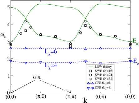
Figure 4: The two types of excitations in the Compass-Heisenberg model: spin-wave excitations (SWE) with the lowest energies for clusters of $N=16,24,32$ sites (squares, circles and diamonds); the LSW dispersion Eq. (8) shown by solid lines, with minima $E_{a}$ at ${\bf k}=(0,0)$ and ${\bf k}=(\pi,\pi)$), see Eq. (9); and column-flip excitations (CFE) with energies $E_{c}$ (triangles) for two values of $L_{z}=4,6$ (with $L_{x}=4$), see Eq. (10). Parameters $I=0.1J_{c}$ and $\phi=3\pi/20$ are corresponding to $G_{z}$ phase in Fig. 1.

For finite clusters and for small enough $I/J_{z}$ excitations to other compass states have lower energies than the spin waves. The simplest ones of these excitations, called column flip, consist of reversing all spins of a single column — these excitations are fundamentally different from spin waves which occur for Heisenberg systems with long range order. The resulting excitation energy is mainly due to Heisenberg couplings between each spin of the column and its two horizontal neighbours, and is given by

$$E_{c}\simeq 4L_{z}|I|,$$ (10)

thus increasing linearly with column size. The smallness of the coupling $J_{\rm col}$ Eq. (5) between columns gives rather weak $\bf{k}$-dependence of these excitations, as shown in Fig. 4 for $L_{z}=4$ and fixed $L_{x}=4$. This coupling decreases with increasing column length, being $J_{\rm col}=2.3\times 10^{-3}$ for $L_{z}=4$ and $J_{\rm col}=1.2\times 10^{-4}$ for $L_{z}=6$ (both with $\phi=3\pi/20$) — thus almost no dispersion is seen for $L_{z}=6$. These excitations are shifted above the spin-wave ones with increasing size $L_{z}$ and play no role in the thermodynamic limit.

A comparison of the column-flip excitations with spin waves is of importance for finite clusters since such column flips could be used for fault-tolerant quantum computing, where a qubit would be encoded in the orientation of a given spin column. A criterion for the use of such a device is that spin-wave excitation energies remain above those of column flips, i.e., $E_{a}>E_{c}$, which defines a column-flip regime. In Fig. 5 we present regimes of these distinct excitations obtained for three clusters in the case of AF interactions, with fixed number of $L_{x}=4$ columns and increasing column length $L_{z}=2,4,6$. On the one hand, the size of columns and the anisotropy ratio $J_{x}/J_{z}$ determine the range of the column-flip regime, which requires large coupling anisotropy (small $J_{x}/J_{z}$) and sufficiently short columns (since $E_{c}\propto L_{z}$). In the perturbative regime of small $I/J_{z}$ and $J_{x}/J_{z}$ one finds the transition between these two distinct regimes at

$$L_{z}I=\sqrt{J_{z}(J_{z}-J_{x})}+f_{L}\,.$$ (11)

The factor $f_{L}$, accounting for finite-size corrections to the spin-wave dispersion, vanishes in the thermodynamic limit; but remarkably, even in the vicinity of the isotropic point ($J_{x}\leq J_{z}$), these corrections allow compass excitations to be the lowest ones for small enough $L_{z}|I|$. On the other hand, $L_{z}$ must be large enough for column-flip excitations of different columns to be sufficiently far from one another in Hilbert space, so that qubits remain well protected against local fluctuations and noise [6]. Thus, for given values of $\{J_{x},J_{z}\}$ couplings the system size must correspond to a compromise between all constraints above, in order to define correctly qubits with help of these column-flip excitations.

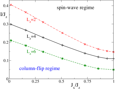
Figure 5: Two distinct regimes of low energy excitations for $J_{x}<J_{z}$ [25]: column-flip regime with $E_{a}>E_{c}$ (lower part) and spin-wave regime with $E_{a}<E_{c}$ (upper part), as obtained for $\phi=3\pi/20$ and for $L_{x}\times L_{z}$ clusters with: $L_{x}=4$ and $L_{z}=2,4,6$. For each system size, $E_{a}$ and $E_{c}$ are calculated separately.

In contrast to frequently proposed quantum computing schemes [6, 26], here a column-flip switches between quasi-degenerate eigenstates (split by an energy $\propto J_{\rm col}$); thanks to their columnar character the fault tolerance of the compass model persists, unaltered by perturbating Heisenberg interactions — imperfections in switches should not harm information storage more than usual decoherence sources.

One may also wonder whether the features discussed above are a consequence of the particular nature of perturbing interactions. We can for instance consider, instead of Heisenberg couplings, XY-type couplings — or rather XZ-type within our notation, i.e., introducing $I_{xz}(\sigma_{i}^{x}\sigma_{j}^{x}+\sigma_{i}^{z}\sigma_{j}^{z})$ for each pair of nearest neighbours, such that the $\sigma_{i}^{y}$ spin components do not appear in the Hamiltonian anymore. One finds that the order induced by perturbations at even infinitesimal $I_{xz}$ persists since e.g. the neighbouring columns in column-ordered compass states are again coupled at first order in perturbation. The global phase diagram would mainly differ from that found for the CH model (presented in Fig. 1) by the absence of $F_{y}$ phase, and the transition lines would not be affected by quantum fluctuations at all. Nevertheless, the column flips will also be the lowest energy excitations for sufficiently small perturbation amplitude $I_{xz}$ and system size, allowing here again for a possible design of a quantum computation scheme.

Summarizing, we have shown that the macroscopic $2^{L}$ ground state degeneracy of the anisotropic $L\times L$ compass model is lifted by infinitesimal Heisenberg interaction $I$. The Compass-Heisenberg model has a rich phase diagram — for small $|I|$ long-range order develops from a pair of compass states, and the remaining compass states are split off by an energy $E_{c}\sim 4L|I|$. Thus the spin waves are the lowest energy excitations in a large system. For nanoscale structures of length $L$, however, the sequence of excited states can be reversed, with quasi-degenerate compass states being pushed below the spin-wave excitations, provided the product $L|I|$ is small enough. In this way decoherence of column-flip excitations by decay via spin waves could be avoided in quantum computation applications.

- [1] Kugel K. I. and Khomskii D. I., Sov. Phys. Usp., 25 (1982) 231.
- [2] Feiner L. F., Oleś A. M. and Zaanen J., Phys. Rev. Lett., 78 (1997) 2799.
- [3] Khomskii D. I. and Mostovoy M. V., J. Phys. A, 36 (2003) 9197.
- [4] Nussinov Z., Biskup M., Chayes L. and van den Brink J., Europhys. Lett., 67 (2004) 990.
- [5] Mishra A., Ma M., Zhang F.-C., Guertler S., Tang L.-H. and Wan S., Phys. Rev. Lett., 93 (2004) 207201.
- [6] Douçot B., Feigel’man M. V., Ioffe L. B. and Ioselevich A. S., Phys. Rev. B, 71 (2005) 024505.
- [7] Nussinov Z. and Fradkin E., Phys. Rev. B, 71 (2005) 195120.
- [8] Milman P., Maineult W., Guibal S., Guidoni L., Douçot B., Ioffe L. and Coudreau T., Phys. Rev. Lett., 99 (2007) 020503.
- [9] Gladchenko S., Olaya D., Dupont-Ferrier E., Douçot B., Ioffe L. B. and Gershenson M. E., Nature Physics, 5 (2009) 48.
- [10] Jackeli G. and Khaliullin G., Phys. Rev. Lett., 102 (2009) 017205.
- [11] Kitaev A., Ann. Phys. (N.Y.), 321 (2006) 2.
- [12] Dorier J., Becca F. and Mila F., Phys. Rev. B, 72 (2005) 024448.
- [13] Wenzel S. and Janke W., Phys. Rev. B, 78 (2008) 064402; Wenzel S., Janke W. and Läuchli A. M., Phys. Rev. E, 81 (2010) 066702.
- [14] Chen H.-D., Fang C., Hu J. and Yao H., Phys. Rev. B, 75 (2007) 144401.
- [15] Brzezicki W., Dziarmaga J. and Oleś A. M., Phys. Rev. B, 75 (2007) 134415; Eriksson E. and Johannesson H., Phys. Rev. B, 79 (2009) 224424.
- [16] Orús R., Doherty A. C. and Vidal G., Phys. Rev. Lett., 102 (2009) 077203.
- [17] Cincio L., Dziarmaga J. and Oleś A. M., Phys. Rev. B, 82 (2010) 104416.
- [18] Khaliullin G., Phys. Rev. B, 64 (2001) 212405.
- [19] Brzezicki W. and Oleś A. M., Phys. Rev. B, 82 (2010) 060401.
- [20] Gu Z.-G. and Wen X.-G., Phys. Rev. B, 80 (2009) 155131.
- [21] Dagotto E., Rev. Mod. Phys., 66 (1994) 763.
- [22] For the smallest considered values of , taken finite to define unambiguously the finite-size ground state, behaves as , where is the length of columns.
- [23] Along the line , a transformation gives equal amplitudes () for and terms for a bond connecting sites and . Thus, order parameters of the and phases are related to each other and equal.
- [24] Vidal J., Thomale R., Schmidt K. P. and Dusuel S., Phys. Rev. B, 80 (2009) 081104.
- [25] For one finds equivalent results.
- [26] Kou S.-P., Phys. Rev. A, 80 (2009) 052317.