Asymptotic expansion for the resistance between two maximum separated nodes on a $M\times N$ resistor network

Abstract

We analyze the exact formulae for the resistance between two arbitrary notes in a rectangular network of resistors under free, periodic and cylindrical boundary conditions obtained by Wu [J. Phys. A 37, 6653 (2004)]. Based on such expression, we then apply the algorithm of Ivashkevich, Izmailian and Hu [J. Phys. A 35, 5543 (2002)] to derive the exact asymptotic expansions of the resistance between two maximum separated nodes on an $M\times N$ rectangular network of resistors with resistors $r$ and $s$ in the two spatial directions. Our results is $\frac{1}{s}R_{M\times N}(r,s)=c(\rho)\,\ln{S}+c_{0}(\rho,\xi)+\sum_{p=1}^{\infty}\frac{c_{2p}(\rho,\xi)}{S^{p}}$ with $S=MN$, $\rho=r/s$ and $\xi=M/N$. The all coefficients in this expansion are expressed through analytical functions. We have introduced the effective aspect ratio $\xi_{eff}=\sqrt{\rho}\;\xi$ for free and periodic boundary conditions and $\xi_{eff}=\sqrt{\rho}\;\xi/2$ for cylindrical boundary condition and show that all finite size correction terms are invariant under transformation $\xi_{eff}\to{1}/\xi_{eff}$.

I Introduction

The calculation of the resistance between arbitrary node of infinite networks of resistors is a well studied subject resistor1 ; resistor2 ; resistor3 . Resistor networks have been widely studied as models for conductivity problems and classical transport in disordered media resistor4 ; resistor5 ; resistor6 .

Besides being a central problem in electric circuit theory, the computation of resistances is also relevant to a wide range of problems ranging from random walks (see resistor2 and Lovasz1996 , and discussions below), first-passage processes Redner2001 , to lattice Green’s functions Katsura1971 . Little attention has been paid to finite network, even though the latter are those occurring in real life. Recently, Wu Wu2004 has revisited the two-point resistance problem and deduced a closed-form expression for the resistance between arbitrary two nodes for finite networks with resistors $r$ and $s$ in the two spatial directions. Later, Jafarizadeh, et.al. Jafar2007 proposed an algorithm for the calculation of the resistance between two arbitrary nodes in an arbitrary distance-regular networks. However, the exact expression obtained in Wu2004 is in the form of a double summation whose mathematical and physical contents are not immediately apparent. Quite recently Essam and Wu based on the exact expression for the resistance between arbitrary two nodes for finite rectangular network obtained in Wu2004 has derived the asymptotic expansion for the corner-to-corner resistance $(R_{M\times N}(r,s))$ on an $M\times N$ rectangular resistor network under free boundary conditions. For the case $M=N$ and $r=s=1$ they computed the finite-size corrections to the corner-to-corner resistance up to order $N^{-4}$:

$$R_{N\times N}(1,1)=\frac{4}{\pi}\log N+0.077\,318+\frac{0.266\,070}{N^{2}}-\frac{0.534\,779}{N^{4}}+O\left(\frac{1}{N^{6}}\right).$$

The computation of the asymptotic expansion of the corner-to-corner resistance (in other word the resistance between two maximum separated nodes) of a rectangular resistor network has been of interest for some time, as its value provides a lower bound to the resistance of compact percolation clusters in the Domany-Kinzel model of a directed percolation Domany1984 .

In experiments and in numerical studies of model systems, it is essential to take into account finite size effects in order to extract correct infinite-volume predictions from the data. As soon as one has a finite system one must consider the question of boundary conditions on the outer surfaces or “walls” of the system. The systems under various boundary conditions have the same per-site free energy, internal energy, specific heat, etc, in the bulk limit, whereas the finite size corrections are different. To understand the effects of boundary conditions on finite-size scaling and finite-size corrections, it is valuable to study model systems. Therefore, in recent decades there have many investigations on finite-size scaling, finite-size corrections, and boundary effects for model systems Blote ; Cardy1 ; huetal ; izmailian2002 ; izmailian2002a ; izmailian2003 ; izmailian2007 ; EssamWu2009 . Of particular importance in such studies are exact results where the analysis can be carried out without numerical errors.

In this paper we will derive the exact asymptotic expansions for resistance between two maximum separated nodes on the rectangular network under free, periodic and cylindrical boundary conditions. We will show that the exact asymptotic expansion of the resistance between nodes of the network for all boundary conditions can be written as

$$\frac{1}{s}R_{M\times N}(r,s) = c(\rho)\,\ln{S}+c_{0}(\rho,\xi)+\sum_{p=1}^{\infty}\frac{c_{2p}(\rho,\xi)}{S^{p}}$$ (1)

where $\rho=r/s$, $S=MN$ is the area of the lattice and $\xi=M/N$ is the aspect ratio. The all coefficients in this expansion are expressed through analytical functions. We will show that all finite size correction terms are invariant under transformation $\xi\to{1}/({\rho\;\xi})$ for free and periodic boundary conditions and under transformation $\xi\to 4/({\rho\;\xi})$ for cylindrical boundary condition, which actually means that $\xi_{eff}$

$$\xi_{eff} = \xi\;\sqrt{\rho}\qquad\mbox{for free and periodic b.c.}$$ (2)

$$\xi_{eff} = \xi\;\sqrt{\rho}/2\qquad\mbox{for cylindrical b.c.}$$ (3)

can be regarded as the effective aspect ratio.

The organization of this paper is as follows: Based on the exact expression for the resistance between arbitrary two nodes for finite rectangular network under free, periodical and cylindrical boundary conditions obtained in Wu2004 we express the resistance between two most separated nodes in terms of $G_{\alpha,\beta}(\rho,\xi)$ with $(\alpha,\beta)=(1/2,0)$ and $(0,1/2)$ (Sec. II). We then extend Ivashkevich, Izmailian and Hu algorithm izmailian2002 to derive the exact asymptotic expansions of the resistance between two maximum separated nodes on the rectangular network for all boundary conditions and write down the expansion coefficients up to the second order (Sec. III). We also discuss our results in Sec. IV.

II Two-dimensional resistor networks

An electrical network can be regarded as a graph in which the resistance $R_{ij}$ is associated to the edge between pair of connected nodes i and j. Denote the electric potential at the i-th vertex by $V_{i}$ and the net current flowing into the network at the i-th vertex by $I_{i}$. When the potential difference occurs between points i and j, the current is given by the Ohm’s law $I_{ij}=(V_{i}-V_{j})C_{ij}$, where $C_{ij}=1/R_{ij}$ is the conductance of the respective link. By the Kirchhoff’s current law total current outflow from any point in the interior is zero, $\sum_{j}I_{ij}=0$, we then find for the voltage

$$V_{i}=\sum_{j}V_{j}C_{ij}/C_{i}$$ (4)

where $C_{i}=\sum_{j}C_{ij}$ and the sum is over all nodes j which are connected to i.

The two-point resistance has a probabilistic interpretation based on classical random walker walking on the network. The averaging property expressed by equation (4) implies that the voltage is a harmonic function on the interior points of the graph. This makes the basis for the probabilistic interpretation of the voltage Ballobas1998 ; resistor2 ; Kemeny1976 ; Kelly1979 . The random walk determined by the electrical network is defined as finite state Markov chain (for more details see resistor2 )with the transition probabilities $P_{ij}$ that are weighted with the conductances as $P_{ij}=C_{ij}/C_{i}$. Then, when the constant voltage is applied to the graph such that $V_{a}=1$ and $V_{b}=0$, the voltage in an interior point x is determined as the hitting probability $h_{x}$ that a walker staring at x reaches the point a before reaching b.

Consider a rectangular $M\times N$ network of resistors with resistances r and s on edges of the network in the respective horizontal and vertical directions. The closed-form expression for the resistance $R_{\{M\times N\}}({\bf r}_{1},{\bf r}_{2})$ between arbitrary two nodes ${\bf r}_{1}=(x_{1},y_{1})$ and ${\bf r}_{2}=(x_{2},y_{2})$ for free, periodic and cylindrical boundary conditions was obtained in Wu2004 .

In what follows, we will show that the resistance $R_{\{M\times N\}}(r,s)$ between two maximum separated nodes of the network for all above mentioned boundary conditions can be expressed in terms of $G_{\alpha,\beta}(\rho,M,N)$ only,

$$R_{M\times N}^{\,\rm free}(r,s) = -r+\frac{\sqrt{rs}}{S}\left(G_{0,1/2}(\rho,M,N)+G_{1/2,0}(\rho,M,N)\right),$$ (5)

$$R_{M\times N}^{\rm per}(r,s) = \frac{\sqrt{rs}}{S}\left(G_{0,1/2}(\rho,M/2,N/2)+G_{1/2,0}(\rho,M/2,N/2\right),$$ (6)

$$R_{M\times N}^{\rm cyl}(r,s) = \frac{\sqrt{rs}}{S}\left(G_{0,1/2}(\rho,M/2,N)+G_{1/2,0}(\rho,M/2,N)\right),$$ (7)

where $G_{\alpha,\beta}(\rho,\xi)$ is given by

$$G_{\alpha,\beta}(\rho,M,N)=M\;{\tt~{}Re}\sum_{n=0}^{N-1}f\left(\pi\frac{n+\alpha}{N}\right)\;{\rm coth}\left[M\,\omega\left(\pi\frac{n+\alpha}{N}\right)+i\pi\beta\right]$$ (8)

for $(\alpha,\beta)\neq(0,0)$. The function $\omega(x)$ is the same for all boundary conditions and given by:

$$\omega(x)={\rm arcsinh}\sqrt{\rho}\sin x$$ (9)

and function $f(x)$ is depend on boundary conditions and given by

$$f(x) = \frac{\cos^{2}x\sqrt{1+\rho\sin^{2}x}}{\sin x}\qquad\quad\mbox{for free BCs,}$$ (10)

$$f(x) = \frac{1}{\sin x\,\sqrt{1+\rho\sin^{2}x}}\qquad\quad\mbox{for periodic BCs,}$$ (11)

$$f(x) = \frac{\cos^{2}x}{\sin x\,\sqrt{1+\rho\sin^{2}x}}\qquad\quad\mbox{for cylindrical BCs}$$ (12)

II.1 Two-dimensional network: free boundary conditions

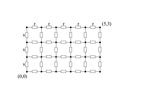
Figure 1: A $6\times 4$ rectangular network with free boundary conditions

Consider a rectangular $M\times N$ network of resistors with free boundary conditions and with resistances r and s on edges of the network in the respective horizontal and vertical directions. The example of a rectangular network with $M=6$, $N=4$ is shown in Fig. 1. The resistance between the two maximum separated nodes on the network of resistors with free boundary conditions is the resistance between opposite corner nodes $(0,0)$ and $(M-1,N-1)$ of the network which is given by EssamWu2009

$$R_{M\times N}^{free}(r,s) = \frac{r(M-1)}{N}+\frac{s(N-1)}{M}$$

$$+ \frac{2}{MN}\sum_{m=1}^{M-1}\sum_{n=1}^{N-1}\frac{\left[\cos(\theta_{m}/2)\cos(\phi_{n}/2)-\cos\left(M-\frac{1}{2}\right)\theta_{m}\cos\left(N-\frac{1}{2}\right)\phi_{n}\right]^{2}}{r^{-1}(1-\cos\theta_{m})+s^{-1}(1-\cos\phi_{n})}$$

where $\theta_{m}=\pi m/M,\phi_{n}=\pi n/N$. With the help of the identity

$$\sum_{n=0}^{N/2-1}\cot^{2}\frac{\pi(n+1/2)}{N}=\frac{N(N-1)}{2}$$ (14)

the Eq. (II.1) can be rewritten in the following form

$$R_{M\times N}^{free}(r,s) = -\frac{r(M-1)}{N}-\frac{s(N-1)}{M}$$

$$+ \frac{2}{MN}\sum_{m=0}^{M-1}\sum_{\begin{subarray}{c}n=0\\ (m,n)\neq(0,0)\end{subarray}}^{N-1}\frac{\left[\cos(\theta_{m}/2)\cos(\phi_{n}/2)-\cos\left(M-\frac{1}{2}\right)\theta_{m}\cos\left(N-\frac{1}{2}\right)\phi_{n}\right]^{2}}{r^{-1}(1-\cos\theta_{m})+s^{-1}(1-\cos\phi_{n})}$$

Using the fact that $\cos\left(M-\frac{1}{2}\right)\theta_{m}=(-1)^{m}\cos(\theta_{m}/2)$ and $\cos\left(N-\frac{1}{2}\right)\phi_{n}=(-1)^{n}\cos(\phi_{n}/2)$ the Eq. (II.1) can be rewritten in the following form

$$R_{M\times N}^{free}(r,s) = -\frac{r(M-1)}{N}-\frac{s(N-1)}{M}$$

$$+ \frac{4r}{MN}\sum_{m=0}^{M-1}\sum_{\begin{subarray}{c}n=0\\ m+n=odd\end{subarray}}^{N-1}\frac{\cos^{2}(\phi_{n}/2)\left(1+\rho\sin^{2}(\phi_{n}/2)\right)}{\sin^{2}(\theta_{m}/2)+\rho\sin^{2}(\phi_{n}/2)}$$

$$- \frac{4r}{MN}\sum_{m=0}^{M-1}\sum_{\begin{subarray}{c}n=0\\ m+n=odd\end{subarray}}^{N-1}\cos^{2}(\phi_{n}/2)$$

There are two possibilities for the restriction $m+n=$ odd to hold, namely, m-odd, n-even and m-even, n-odd. Splitting the sum into two parts accordingly we obtain

$$R_{M\times N}^{free}(r,s) = -\frac{r(M-1)}{N}-\frac{s(N-1)}{M}$$

$$+ \frac{4r}{MN}\sum_{m=0}^{M/2-1}\sum_{n=0}^{N/2-1}\left[f(m+1/2,n)+f(m,n+1/2)\right]$$

$$- \frac{4r}{MN}\sum_{m=0}^{M/2-1}\sum_{n=0}^{N/2-1}\cos^{2}\frac{\pi n}{N}-\frac{4r}{MN}\sum_{m=0}^{M/2-1}\sum_{n=0}^{N/2-1}\cos^{2}\frac{\pi(n+1/2)}{N}$$

where

$$f(m,n)=\frac{\cos^{2}\frac{\pi n}{N}\left(1+\rho\sin^{2}\frac{\pi n}{N}\right)}{\sin^{2}\frac{\pi m}{M}+\rho\sin^{2}\frac{\pi n}{N}}.$$ (18)

Sums of the term $\cos^{2}(x)$ can be carried out using the identities

$$\sum_{n=0}^{N/2-1}\cos^{2}\frac{\pi n}{N}=\frac{N}{4}+\frac{1}{2},\qquad\sum_{n=0}^{N/2-1}\cos^{2}\frac{\pi(n+1/2)}{N}=\frac{N}{4}$$ (19)

This yields

$$R_{M\times N}^{free}(r,s) = -\frac{r(M+N)}{N}-\frac{s(N-1)}{M}$$

$$+ \frac{4r}{MN}\sum_{m=0}^{M/2-1}\sum_{n=0}^{N/2-1}\left[f(m+1/2,n)+f(m,n+1/2)\right]$$

Now we first express double sums $\sum_{n=0}^{N/2-1}\sum_{m=0}^{M/2-1}f(m,n)$ in terms of $\sum_{n=0}^{N-1}\sum_{m=0}^{M-1}f(m,n)$, It it easy to show that $f(m,N-n)=f(M-m,n)=f(m,n)$ and thus

$$2 \sum_{n=0}^{N/2-1}\sum_{m=0}^{M/2-1}\left[f(m+1/2,n)+f(m,n+1/2)\right]=\frac{1}{2}\sum_{n=0}^{N-1}\sum_{m=0}^{M-1}\left[f(m+1/2,n)+f(m,n+1/2)\right]$$ (21)

$$- \sum_{n=0}^{N/2-1}\left[f(M/2,n+1/2)-f(0,n+1/2)\right]-\sum_{m=0}^{M/2-1}\left[f(m+1/2,N/2)-f(m+1/2,0)\right].$$

With the help of the identities given by Eq. (14) and

$$\sum_{m=0}^{M/2-1}\frac{1}{\sin^{2}\frac{\pi(m+1/2)}{M}}=\frac{M^{2}}{2}$$ (22)

The sums $\sum_{n=0}^{N/2-1}\left[f(M/2,n+1/2)-f(0,n+1/2)\right]$ , $\sum_{m=0}^{M/2-1}\left[f(m+1/2,N/2)+f(m+1/2,0)\right]$ can be written as

$$\sum_{n=0}^{N/2-1}\left[f(M/2,n+1/2)-f(0,n+1/2)\right] = -\frac{1}{\rho}\sum_{n=0}^{N/2-1}\cot^{2}\frac{\pi(n+1/2)}{N}=-\frac{N(N-1)}{2\rho}$$

$$\sum_{m=0}^{M/2-1}\left[f(m+1/2,N/2)-f(m+1/2,0)\right] = -\sum_{m=0}^{M/2-1}\frac{1}{\sin^{2}\frac{\pi(m+1/2)}{M}}=-\frac{M^{2}}{2}.$$ (23)

Plugging Eqs. (21) and (23) back in Eq. (II.1) we finally obtain

$$R_{M\times N}^{free}(r,s) = -r+\frac{r}{MN}\sum_{m=0}^{M-1}\sum_{n=0}^{N-1}\left[f(m+1/2,n)+f(m,n+1/2)\right]$$

$$= -r+\frac{r}{MN}\sum_{n=0}^{N-1}\left(1+\rho\sin^{2}\frac{\pi n}{N}\right)\cos^{2}\frac{\pi n}{N}\,\sum_{m=0}^{M-1}\Big{[}{\rho\sin^{2}\frac{\pi n}{N}+\sin^{2}\frac{\pi(m+\frac{1}{2})}{M}}\Big{]}^{-1}$$

$$+ \frac{r}{MN}\sum_{n=0}^{N-1}\left(1+\rho\sin^{2}\frac{\pi(n+1/2)}{N}\right)\cos^{2}\frac{\pi(n+1/2)}{N}$$

$$\times \sum_{m=0}^{M-1}\Big{[}{\rho\sin^{2}\frac{\pi(n+1/2)}{N}+\sin^{2}\frac{\pi m}{M}}\Big{]}^{-1}$$

The sum over m in the Eq. (II.1) can be carried out using the identity GradshteinRyzhik

$$\prod_{m=0}^{M-1}4\textstyle{\left[~{}\!{\rm sinh}^{2}\omega+\sin^{2}\frac{\pi(m+\beta)}{M}\right]}=4\left|~{}\!{\rm sinh}\left(M\omega+i\pi\beta\right)\right|^{2}$$ (25)

Note that using more complicated approach the identity given by Eq. (25) has been obtained previously in EssamWu2009 and Janke1 .

Taking the derivative over $\omega$ from the logarithm of the left and right side of the equation (25) we obtain

$$\sum_{m=0}^{M-1}\Big{[}{{\rm sinh}^{2}\omega+\sin^{2}\frac{(m+\beta)\pi}{M}}\Big{]}^{-1}=2M\,{\tt~{}Re}\frac{{\rm coth}\left[M\,\omega+i\pi\beta\right]}{{\rm\sinh 2\omega}}.$$ (26)

Thus the sum over m in the Eq. (II.1) can be carried out as

$$\sum_{m=0}^{M-1}\Big{[}{\rho\sin^{2}\frac{\pi n}{N}+\sin^{2}\frac{\pi(m+\frac{1}{2})}{M}}\Big{]}^{-1}=2M\,{\tt~{}Re}\frac{{\rm coth}\left[M\,\omega(\frac{\pi n}{N})+i\pi/2\right]}{{\rm\sinh 2\omega(\frac{\pi n}{N})}}$$ (27)

$$\sum_{m=0}^{M-1}\Big{[}{\rho\sin^{2}\frac{\pi(n+1/2)}{N}+\sin^{2}\frac{\pi m}{M}}\Big{]}^{-1}=2M\,{\tt~{}Re}\frac{{\rm coth}M\,\omega(\frac{\pi(n+1/2)}{N})}{{\rm\sinh 2\omega(\frac{\pi(n+1/2)}{N})}}$$ (28)

where $\omega(x)$ is given by Eq. (66). It is easy to see that

$${\rm\sinh 2\omega}(x)=2\sqrt{\rho}\sin{x}\sqrt{1+\rho\sin{x}^{2}}$$ (29)

Plugging Eqs. (27) and (28) back in Eq. (II.1) we obtain that $R_{M\times N}^{free}(r,s)$ can be written in the form given by Eq. (5).

II.2 Two-dimensional network: periodical boundary conditions

Consider a rectangular $M\times N$ resistor network with periodic boundary conditions. Using a closed-form expression for the resistance between arbitrary two nodes for finite network given by Eq. (43) of Wu2004 we can obtain for the resistance between nodes $r_{1}=(0,0)$ and $r_{2}=(M/2,N/2)$ of the network the following expression

$$R_{M\times N}^{\rm per}(r,s)=\frac{1}{MN}\,{\sum_{m=0}^{M-1}\sum_{\begin{subarray}{c}n=0\\ (m,n)\neq(0,0)\end{subarray}}^{N-1}\frac{1-\cos\left(M\theta_{m}+N\phi_{n}\right)}{r^{-1}(1-\cos 2\theta_{m})+s^{-1}(1-\cos 2\phi_{n})}},$$ (30)

Using the fact that $\cos\left(M\theta_{m}+N\phi_{n}\right)=(-1)^{m+n}$ the Eq. (30) can be rewritten in the following form

$$R_{M\times N}^{\rm per}(r,s)=\frac{r}{MN}\sum_{m=0}^{M-1}\sum_{\begin{subarray}{c}n=0\\ m+n=odd\end{subarray}}^{N-1}\frac{1}{\sin^{2}\theta_{m}+\rho\sin^{2}\phi_{n}}$$ (31)

Splitting the sum into two parts accordingly we obtain

$$R_{M\times N}^{per}(r,s) = \frac{r}{MN}\sum_{m=0}^{M/2-1}\sum_{n=0}^{N/2-1}\frac{1}{\sin^{2}\left(\frac{2\pi(m+1/2)}{M}\right)+\rho\sin^{2}\left(\frac{2\pi n}{N}\right)}$$ (32)

$$+ \frac{r}{MN}\sum_{m=0}^{M/2-1}\sum_{n=0}^{N/2-1}\frac{1}{\sin^{2}\left(\frac{2\pi m}{M}\right)+\rho\sin^{2}\left(\frac{2\pi(n+1/2)}{N}\right)}$$

The sum over m in the Eq. (32) can be carried out using the identities given by Eq. (27) and (28). This yields

$$R_{M\times N}^{per}(r,s) = \frac{\sqrt{rs}}{N}\sum_{n=0}^{N/2-1}\frac{{\rm coth}\left[M\,\omega\left(\frac{2\pi n}{N}\right)+i\pi/2\right]}{\sin\frac{2\pi n}{N}\sqrt{1+\rho\sin^{2}{\frac{2\pi n}{N}}}}$$

$$+ \frac{\sqrt{rs}}{N}\sum_{n=0}^{N/2-1}\frac{{\rm coth}M\,\omega\left(\frac{2\pi(n+1/2)}{N}\right)}{\sin\frac{2\pi(n+1/2)}{N}\sqrt{1+\rho\sin^{2}{\frac{2\pi(n+1/2)}{N}}}}.$$

Introducing function $f(x)$ given by Eq. (11) we finally arrived to the Eq. (6).

II.3 Two-dimensional network: cylindrical boundary conditions

Consider a rectangular $M\times N$ resistor network embedded on a cylinder with periodic boundary in the direction of M and free boundaries in the direction of N. Using Eq. (46) of Wu2004 , the resistance between nodes $r_{1}=(0,0)$ and $r_{2}=(M/2,N-1)$ of the network is

$$R_{M\times N}^{\rm cyl}(r,s)=-\frac{rM}{4N}$$ (34)

$$+\frac{1}{MN}\,{\sum_{m=0}^{M-1}\sum_{\begin{subarray}{c}n=0\\ (m,n)\neq(0,0)\end{subarray}}^{N-1}\Bigg{(}\frac{\cos^{2}\left(\frac{1}{2}\phi_{n}\right)+\cos^{2}\left(N-\frac{1}{2}\right)\phi_{n}-2\cos\left(\frac{1}{2}\phi_{n}\right)\cos\left(N-\frac{1}{2}\right)\phi_{n}\cos M\theta_{m}}{r^{-1}(1-\cos 2\theta_{m})+s^{-1}(1-\cos\phi_{n})}}\Bigg{)}.$$

Using the fact that $\cos\left(M\theta_{m}\right)=(-1)^{m}$ and $\cos\left(N-\frac{1}{2}\right)\phi_{n}=(-1)^{n}\cos(\phi_{n}/2)$ the Eq. (34) can be rewritten in the following form

$$R_{M\times N}^{\rm cyl}(r,s)=-\frac{rM}{4N}+\frac{2r}{MN}\sum_{m=0}^{M-1}\sum_{\begin{subarray}{c}n=0\\ m+n=odd\end{subarray}}^{N-1}\frac{\cos^{2}(\phi_{n}/2)}{\sin^{2}\theta_{m}+\rho\sin^{2}(\phi_{n}/2)}$$ (35)

Splitting the sum into two parts accordingly we obtain

$$R_{M\times N}^{\rm cyl}(r,s) = -\frac{rM}{4N}+\frac{2r}{MN}\sum_{m=0}^{M/2-1}\sum_{n=0}^{N/2-1}\frac{\cos^{2}\frac{\pi n}{N}}{\sin^{2}\frac{2\pi(m+1/2)}{M}+\rho\sin^{2}\frac{\pi n}{N}}$$

$$+ \frac{2r}{MN}\sum_{m=0}^{M/2-1}\sum_{n=0}^{N/2-1}\frac{\cos^{2}\frac{\pi(n+1/2)}{N}}{\sin^{2}\frac{2\pi m}{M}+\rho\sin^{2}\frac{\pi(n+1/2)}{N}}$$

Following along the same lines as in the case of free boundary conditions the Eq. (II.3) can be written as

$$R_{M\times N}^{\rm cyl}(r,s) = \frac{r}{MN}\sum_{n=0}^{N-1}\cos^{2}\frac{\pi n}{N}\sum_{m=0}^{M/2-1}\frac{1}{\sin^{2}\frac{2\pi(m+1/2)}{M}+\rho\sin^{2}\frac{\pi n}{N}}$$

$$+ \frac{r}{MN}\sum_{n=0}^{N-1}\cos^{2}\frac{\pi(n+1/2)}{N}\sum_{m=0}^{M/2-1}\frac{1}{\sin^{2}\frac{2\pi m}{M}+\rho\sin^{2}\frac{\pi(n+1/2)}{N}}$$

The sum over m in the Eq. (II.3) can be carried out using the identities given by Eq. (27) and (28). This yields

$$R_{M\times N}^{cyl}(r,s) = \frac{\sqrt{rs}}{2N}\sum_{n=0}^{N-1}\frac{\cos^{2}{\frac{\pi n}{N}}}{\sin\frac{2\pi n}{N}\sqrt{1+\rho\sin^{2}{\frac{2\pi n}{N}}}}{\rm coth}\left[\frac{M}{2}\,\omega\left(\frac{2\pi n}{N}\right)+i\pi/2\right]$$

$$+ \frac{\sqrt{rs}}{2N}\sum_{n=0}^{N-1}\frac{\cos^{2}{\frac{\pi(n+1/2)}{N}}}{\sin\frac{2\pi(n+1/2)}{N}\sqrt{1+\rho\sin^{2}{\frac{2\pi(n+1/2)}{N}}}}{\rm coth}\frac{M}{2}\,\omega\left(\frac{2\pi(n+1/2)}{N}\right).$$

Introducing function $f(x)$ given by Eq. (12) we finally arrived to the Eq. (7).

III Asymptotic expansion of $R_{M\times N}(r,s)$

In Sec. II we have shown that the resistance between two maximum separated nodes on an $M\times N$ rectangular network of resistors with various boundary conditions can be expressed, in terms of the function $G_{1/2,0}(\rho,M,N)$ and $G_{0,1/2}(\rho,M,N)$ only, (see Eqs.(5), (6) and (7)).

Based on such results, one can use the method proposed by Ivashkevich, Izmailian, and Hu izmailian2002 to derive the asymptotic expansion of the $G_{\alpha,\beta}(\rho,M,N)$ in terms so-called Kronecker’s double series Weil , which are directly related to elliptic $\theta$ functions (see Appendix A).

After reaching this point, one can easily write down all the terms of the exact asymptotic expansion for the resistance between two maximum separated nodes of the network ($R_{M\times N}(r,s)$) using Eq. (A). We have found that the exact asymptotic expansion of the $R_{M\times N}(r,s)$ for free, periodic and cylindrical boundary conditions can be written as Eq. (1).

(i) For the free boundary conditions we obtain

$$\frac{1}{s}R_{M\times N}^{free}(r,s) = \frac{2\sqrt{\rho}}{\pi}\left[2\ln{N}+\int_{0}^{\pi}\!\!\varphi(x)~{}\!{\rm d}x+2C_{E}+4\ln{2}-\frac{\pi\sqrt{\rho}}{2}-2\ln{\theta_{2}(i\sqrt{\rho}\,\xi)\theta_{4}(i\sqrt{\rho}\,\xi)}\right]$$ (39)

$$- \frac{\sqrt{\rho}}{\pi}\sum_{p=1}^{\infty}\left(\frac{\pi^{2}\xi}{S}\right)^{p}\frac{\Omega_{2p}}{p(2p)!}\left[{\rm K}_{2p}^{0,1/2}(i\sqrt{\rho}\,\xi)+{\rm K}_{2p}^{1/2,0}(i\sqrt{\rho}\,\xi)\right]$$

where integral $\int_{0}^{\pi}\!\!\varphi(x)~{}\!{\rm d}x$ is given by Eq. (71).

Thus, the coefficients $c_{2p}(\rho,\xi)$ (p=1,2,..) in the expansion Eq. (1) explicitly given by

$$c_{2p}(\rho,\xi)=\frac{\pi^{2p-1}\xi^{p}\sqrt{\rho}}{p(2p)!}\Omega_{2p}\left[{\rm K}_{2p}^{0,1/2}(i\sqrt{\rho}\,\xi)+{\rm K}_{2p}^{1/2,0}(i\sqrt{\rho}\,\xi)\right]$$ (40)

where the differential operators $\Omega_{2p}$ is given by Eq. ( A) and $K_{2p}^{0,1/2}(i\sqrt{\rho}\xi)$, $K_{2p}^{1/2,0}(i\sqrt{\rho}\xi)$ are the Kronecker’s double series which can all be expressed in terms of the elliptic $\theta_{k}(i\sqrt{\rho}\xi)$ ($k=2,3,4$) functions only (see Appendix D).

Here we list the first few coefficients in the expansion given by Eq. (1)

$$c(\rho) = \frac{2\sqrt{\rho}}{\pi}$$ (41)

$$c_{0}(\rho,\xi) = \frac{2\sqrt{\rho}}{\pi}\left(2\ln{\frac{8}{\pi}}+2C_{E}-1-\ln{\xi(1+\rho)-\frac{\pi\sqrt{\rho}}{2}+\frac{\rho-1}{\sqrt{\rho}}}{\rm arctan}\sqrt{\rho}-2\ln{\theta_{2}\theta_{4}}\right)$$ (42)

$$c_{2}(\rho,\xi) = \frac{\pi\tau_{0}}{72}\left(5-3\rho+(1+\rho)\tau_{0}\frac{\partial}{\partial\tau_{0}}\right)(\theta_{4}^{4}-\theta_{2}^{4})$$

$$= \frac{\pi\tau_{0}}{72}\left((5-3\rho)(\theta_{4}^{4}-\theta_{2}^{4})+\pi\tau_{0}(1+\rho)\theta_{3}^{4}\theta_{4}^{4}+4\tau_{0}(1+\rho)(\theta_{4}^{4}-\theta_{2}^{4})\frac{\partial}{\partial\tau_{0}}\ln{\theta_{2}}\right)$$

$$\vdots$$

To simplify the notation we have use the short hand

$$\theta_{k}=\theta_{k}(i\tau_{0}),\qquad k=2,3,4,$$ (44)

where $\tau_{0}=\xi\sqrt{\rho}$.

We have also used the following relations between derivatives of the elliptic functions

$$\frac{\partial}{\partial\tau_{0}}\ln{{\theta}_{3}}=\frac{\pi}{4}{\theta}_{4}^{4}+\frac{\partial}{\partial\tau_{0}}\ln{{\theta}_{2}}\qquad\mbox{and}\qquad\frac{\partial}{\partial\tau_{0}}\ln{{\theta}_{4}}=\frac{\pi}{4}{\theta}_{3}^{4}+\frac{\partial}{\partial\tau_{0}}\ln{{\theta}_{2}}$$

Note that elliptic functions ${\theta}_{2},{\theta}_{3},{\theta}_{4}$ can be expressed through the complete elliptic integral of the first kind $K=K(k)$ and second kind $E=E(k)$ as

$${\theta}_{2}=\sqrt{\frac{2kK(k)}{\pi}},\qquad{\theta}_{3}=\sqrt{\frac{2K(k)}{\pi}},\qquad{\theta}_{4}=\sqrt{\frac{2k^{\prime}K(k)}{\pi}}$$ (45)

where

$$K(k) = \int_{0}^{\pi/2}\frac{{\rm d}x}{\sqrt{1-k^{2}\sin^{2}{x}}},$$ (46)

$$E(k) = \int_{0}^{\pi/2}\sqrt{1-k^{2}\sin^{2}{x}}~{}\!{\rm d}x.$$ (47)

With the help of the identities

$$\frac{\partial}{\partial\tau_{0}}\ln{\theta_{2}}=-\frac{1}{2}{\theta}_{3}^{2}E,\qquad\mbox{and}\qquad\frac{\partial E}{\partial\tau_{0}}=\frac{\pi^{2}}{4}{\theta}_{3}^{2}{\theta}_{4}^{4}-\frac{\pi}{2}{\theta}_{4}^{4}E$$

one can express all derivatives of the elliptic functions in terms of the elliptic functions ${\theta}_{2},{\theta}_{3},{\theta}_{4}$ and the complete elliptic integral of the second kind $E=E(k)$.

For the case $M=N$ and $r=s$ ($\xi=1,\rho=1$) we reproduced the result of Essam and Wu EssamWu2009 :

$$\frac{1}{s}R_{N\times N}^{free}(s,s)=\frac{4}{\pi}\ln{N}+c_{0}+\frac{c_{2}}{N^{2}}+...$$ (48)

with $c_{0}=0.07731889390945876...$ and $c_{2}=0.26607044163847837...$.

(ii) For the periodic boundary conditions we obtain

$$\frac{1}{s}R_{M\times N}^{tor}(r,s) = \frac{\sqrt{\rho}}{2\pi}\left[2\ln{\frac{N}{2}}+\int_{0}^{\pi}\!\!\varphi(x)~{}\!{\rm d}x+2C_{E}+4\ln{2}-2\ln{\theta_{2}(i\sqrt{\rho}\,\xi)\theta_{4}(i\sqrt{\rho}\,\xi)}\right]$$ (49)

$$- \frac{\sqrt{\rho}}{4\pi}\sum_{p=1}^{\infty}\frac{\Omega_{2p}}{p(2p)!}\left(\frac{4\pi^{2}\xi}{S}\right)^{p}\left[{\rm K}_{2p}^{0,1/2}(i\sqrt{\rho}\,\xi)+{\rm K}_{2p}^{1/2,0}(i\sqrt{\rho}\,\xi)\right]$$

where integral $\int_{0}^{\pi}\!\!\varphi(x)~{}\!{\rm d}x$ is given by Eq. (72).

The first few coefficients in the expansion are

$$c(\rho) = \frac{\sqrt{\rho}}{2\pi}$$ (50)

$$c_{0}(\rho,\xi) = \frac{\sqrt{\rho}}{2\pi}\left(2\ln{\frac{4}{\pi}}+2C_{E}-\ln{\xi(1+\rho)}-2\ln{\theta_{2}\theta_{4}}\right)$$ (51)

$$c_{2}(\rho,\xi) = \frac{\pi\tau_{0}}{72}\left(3\rho-1+(1+\rho)\tau_{0}\frac{\partial}{\partial\tau_{0}}\right)(\theta_{4}^{4}-\theta_{2}^{4})$$

$$= \frac{\pi\tau_{0}}{72}\left((3\rho-1)(\theta_{4}^{4}-\theta_{2}^{4})+\pi\tau_{0}(1+\rho)\theta_{3}^{4}\theta_{4}^{4}+4\tau_{0}(1+\rho)(\theta_{4}^{4}-\theta_{2}^{4})\frac{\partial}{\partial\tau_{0}}\ln{\theta_{2}}\right)$$

$$\vdots$$

For the case $M=N$ and $r=s$ ($\xi=1,\rho=1$) we obtain:

$$\frac{1}{s}R_{N\times N}^{tor}(s,s)=\frac{1}{\pi}\ln{N}+c_{0}+\frac{c_{2}}{N^{2}}+...$$ (53)

with $c_{0}=0.2078490664166084...$ and $c_{2}=0.2660704416384784...$.

(iii) And for the cylindrical boundary conditions

$$\frac{1}{s}R_{M\times N}^{cyl}(r,s) = \frac{\sqrt{\rho}}{\pi}\left[2\ln{N}+\int_{0}^{\pi}\!\!\varphi(x)~{}\!{\rm d}x+2C_{E}+4\ln{2}-2\ln{\theta_{2}(i\sqrt{\rho}\,\xi/2)\theta_{4}(i\sqrt{\rho}\,\xi/2)}\right]$$ (54)

$$- \frac{\sqrt{\rho}}{2\pi}\sum_{p=2}^{\infty}\frac{\Omega_{2p}}{p(2p)!}\left(\frac{\pi^{2}\xi}{S}\right)^{p}\left[{\rm K}_{2p}^{0,1/2}(i\sqrt{\rho}\,\xi/2)+{\rm K}_{2p}^{1/2,0}(i\sqrt{\rho}\,\xi/2)\right]$$

where integral $\int_{0}^{\pi}\!\!\varphi(x)~{}\!{\rm d}x$ is given by Eq. (73).

The first few coefficients in the exact asymptotic expansion are

$$c(\rho) = \frac{\sqrt{\rho}}{\pi}$$ (55)

$$c_{0}(\rho,\xi) = \frac{\sqrt{\rho}}{\pi}\left(2\ln{\frac{8}{\pi}}+2C_{E}-\ln{\xi(1+\rho)-\frac{2}{\sqrt{\rho}}}{\rm arctan}\sqrt{\rho}-2\ln{\theta_{2}\theta_{4}}\right)$$ (56)

$$c_{2}(\rho,\xi) = \frac{\pi\tau_{1}}{72}\left(3\rho+5+(1+\rho)\tau_{1}\frac{\partial}{\partial\tau_{1}}\right)(\theta_{4}^{4}-\theta_{2}^{4})$$

$$= \frac{\pi\tau_{1}}{72}\left((5+3\rho)(\theta_{4}^{4}-\theta_{2}^{4})+\pi\tau_{1}(1+\rho)\theta_{3}^{4}\theta_{4}^{4}+4\tau_{1}(1+\rho)(\theta_{4}^{4}-\theta_{2}^{4})\frac{\partial}{\partial\tau_{1}}\ln{\theta_{2}}\right)$$

$$\vdots$$

Here we have use the short hand

$$\theta_{k}=\theta_{k}(i\tau_{1}),\qquad k=2,3,4,$$ (58)

with $\tau_{1}=\xi\sqrt{\rho}/2$.

For the case $M=N$ and $r=s$ ($\xi=1,\rho=1$) we obtain:

$$\frac{1}{s}R_{N\times N}^{cyl}(s,s)=\frac{2}{\pi}\ln{N}+c_{0}+\frac{c_{2}}{N^{2}}+...$$ (59)

with $c_{0}=0.36172475911729557...$ and $c_{2}=-0.28448262410676656...$.

Let us now consider the behavior of the coefficients $c_{2k}(\rho,\xi)$ in the asymptotic expansion of the resistance between two maximum separated nodes on the rectangular network under the Jacobi transformation (see Appendix E). Using Eq. (82) and Eq. (83) we can easily check that $c_{2k}(\rho,\xi)$ (for all k) are invariant under transformation $\tau_{0}\to 1/\tau_{0}$, where

$$\tau_{0} = \xi\;\sqrt{\rho}\qquad\mbox{for free and periodic b.c.}$$ (60)

$$\tau_{0} = \xi\;\sqrt{\rho}/2\qquad\mbox{for cylindrical b.c.}$$ (61)

Using the properties of the $\theta$ -functions and of the functions $K^{\alpha,\beta}_{2p}$ (see Eq. (82) and (83)) we can easily check from Eq. (A) that the $\ln G_{\alpha,\beta}(\rho,M,N)$ have the following behavior under the transformation $\tau_{0}\to 1/\tau_{0}$:

$$G_{1/2,0}(\rho,M,N)\to G_{0,1/2}(\rho,M,N)$$ (62)

Equations (5), (6), (7) and (62) imply that the resistance $R_{\{M\times N\}}(r,s)$ between two maximum separated nodes of the network for all above mentioned boundary conditions is invariant under transformation $\tau_{0}\to 1/\tau_{0}$. This actually means that $\xi_{eff}$ given by Eqs. (2) and (3) can be regarded as the effective aspect ratio.

IV Discussion

In Fig. 2 we plot the conventional aspect-ratio ($\xi$) dependence of the finite-size correction term $c_{0}(\xi)$ for the resistance between two maximum separated nodes on a $M\times N$ resistor network with the free (solid lines), toroidal (dashed lines) and cylindrical (dot-dashed lines) boundary conditions for several values of the factor $\rho$: (a) for $\rho=1$ and (b) for $\rho=4$. We use the logarithmic scales in the horizontal axis. The finite-size correction term $c_{0}(\xi)$ at first decrease until $\xi=\xi_{min}$: $\xi_{min}=1$ for $\rho=1$ and $\xi_{min}=1/2$ for $\rho=4$. Note that $\xi_{min}=1/\sqrt{\rho}$ for arbitrary value of $\rho$. With further increase of $\xi$ it reverses directions, increasing monotonically to infinity. For large enough $\xi$ ($\xi\gg 1$), the finite size properties of the resistor network with cylindrical boundary condition and those of the torus become the same, which means that the boundaries along the shorter direction determine the finite size properties of the system; for both cylindrical boundary condition and the torus, the boundary condition along the shorter direction is the periodic one. For small enough $\xi$ ($\xi\ll 1$), the finite size properties of the resistor network with free boundary condition and those of the cylinder become the same because the boundaries along the shorter directions for these two are the same, that is, the free boundary condition.

Figure 2: Conventional aspect-ratio ($\xi$) dependence of finite-size correction term $c_{0}$ for the resistance between two maximum separated nodes on a $M\times N$ resistor network with the free (solid lines), toroidal (dashed lines) and cylindrical (dot-dashed lines) boundary conditions: (a) for $\rho=1$ and (b) for $\rho=4$. We use the natural logarithmic scales for the horizontal axis.

In Fig. 3 we plot the effective aspect-ratio ($\xi_{eff}$) dependence of the finite-size correction term $c_{0}$ for the resistance between two maximum separated nodes on a $M\times N$ resistor network with the free (solid lines), toroidal (dashed lines) and cylindrical (dot-dashed lines) boundary conditions for several values of the factor $\rho$: (a) for $\rho=1$ and (b) for $\rho=4$. We use the logarithmic scales in the horizontal axis. We can see that finite size correction terms $c_{0}$ are invariant under transformation $\xi_{eff}\to 1/\xi_{eff}$. The finite-size correction term $c_{0}(\xi)$ at first decrease until $\xi_{eff}=1$ for all boundary conditions and for for arbitrary value of $\rho$. With further increase of $\xi_{eff}$ it reverses directions, increasing monotonically to infinity.

Figure 3: Effective aspect-ratio ($\xi_{eff}$) dependence of finite-size correction term $c_{0}$ for the resistance between two maximum separated nodes on a $M\times N$ resistor network with the free (solid lines), toroidal (dashed lines) and cylindrical (dot-dashed lines) boundary conditions: (a) for $\rho=1$ and (b) for $\rho=4$. We use the natural logarithmic scales for the horizontal axis.

In Fig. 4 we plot the $\rho$ dependence of the finite-size correction term $c_{0}(\rho)$ for the resistance between two maximum separated nodes on a $M\times N$ resistor network with the free (solid lines), toroidal (dashed lines) and cylindrical (dot-dashed lines) boundary conditions for several values of the aspect-ratio $\xi$: (a) for $\xi=1$ and (b) for $\xi=4$. The finite-size correction term $c_{0}(\rho)$ at first decrease until $\rho=\rho_{min}$. Note that value of $\rho_{min}$ depends on the boundary conditions as well on the value of the aspect ratio $\xi$. With further increase of $\rho$ it reverses directions, increasing monotonically to infinity.

Figure 4: The ($\rho$) dependence of finite-size correction term $c_{0}$ for the resistance between two maximum separated nodes on a $M\times N$ resistor network with the free (solid lines), toroidal (dashed lines) and cylindrical (dot-dashed lines) boundary conditions: (a) for $\xi=1$ and (b) for $\xi=4$.

In the present paper, we study the two-point resistor problem on planar $M\times N$ rectangular lattices with free, periodic and cylindrical boundary conditions. Using the exact expression for the resistance between arbitrary two nodes for finite rectangular network obtained in Wu2004 and the IIH s algorithm izmailian2002 , we derive the exact asymptotic expansion of the corner-to-corner resistance on the rectangular network for all above mentioned boundary conditions. All corrections to scaling are analytic.

V Acknowledgments

This work was partially supported by the National Science Council of Republic of China (Taiwan) under Grant No. NSC 96-2112-M-033-006. N.Sh.I is supported in part by National Center for Theoretical Sciences: Physics Division, National Taiwan University, Taipei, Taiwan.

Appendix A Asymptotic expansion of $G_{\alpha,\beta}(\rho,{\cal M},{\cal N})$

Using the expansion of the ${\rm coth}x$

$${\rm coth}\,x=1+2\sum_{m=1}^{\infty}e^{-2mx}$$

we can transform the Eq. (8) in the following form

$$G_{\alpha,\beta}(\rho,{\cal M},{\cal N}) = ~{}{\tt Re}{\cal M}\sum_{n=0}^{{\cal N}-1}f\!\left(\textstyle{\frac{\pi(n+\alpha)}{{\cal N}}}\right){\rm coth}\left[{\cal M}f\!\left(\textstyle{\frac{\pi(n+\alpha)}{{\cal N}}}\right)+i\pi\beta\right]$$

$$= {\cal M}\sum_{n=0}^{{\cal N}-1}f\!\left(\textstyle{\frac{\pi(n+\alpha)}{{\cal N}}}\right)+2~{}{\tt Re}{\cal M}\sum_{n=0}^{{\cal N}-1}\sum_{m=1}^{\infty}f\!\left(\textstyle{\frac{\pi(n+\alpha)}{{\cal N}}}\right)e^{-2m\left[{\cal M}\omega\left(\frac{\pi(n+\alpha)}{{\cal N}}\right)+i\pi\beta\right]}$$

where $f(x)$ is given by Eqs. (10), (11) and (12) for free, periodic and cylindrical b.c. respectively.

Using Taylor’s theorem, the asymptotic expansion of the $f(x)$ for all boundary conditions can be written in the following form

$$f(x)=\frac{1}{x}\left[1+\sum_{p=1}^{\infty}\frac{\kappa_{2p}}{(2p)!}x^{2p}\right]$$ (64)

where $\kappa_{2}=\rho-5/3$, $\kappa_{4}=-3\rho^{2}-14\rho+67/15$, etc for free boundary conditions $\kappa_{2}=-\rho+1/3$, $\kappa_{4}=9\rho^{2}+2\rho+7/15$, etc. for periodic boundary conditions and $\kappa_{2}=-\rho-5/3$, $\kappa_{4}=9\rho^{2}+14\rho+67/15$, etc. for cylindrical boundary conditions.

Note that function $f(x)$ can be represent as

$$f(x)=\frac{1}{x}\;\exp\left\{{\sum_{p=1}^{\infty}\frac{\varepsilon_{2p}}{(2p)!}}x^{2p}\right\}$$ (65)

where coefficients $\varepsilon_{2p}$ and $\kappa_{2p}$ are related to each other through relation between moments and cumulants (Appendix B)

$$\kappa_{2} = \varepsilon_{2}$$

$$\kappa_{4} = \varepsilon_{4}+3\varepsilon_{2}^{2}\,$$

$$\vdots$$

We will need also the Taylor expansion of the $\omega(x)$ given by Eq. (9)

$$\omega(x)=x\left(\lambda+\sum_{p=1}^{\infty}\frac{\lambda_{2p}}{(2p)!}\;x^{2p}\right)$$ (66)

where $\lambda=\sqrt{\rho}$, $\lambda_{2}=-\sqrt{\rho}(1+\rho)/3$, $\lambda_{4}=\sqrt{\rho}(1+10\rho+9\rho^{2})/5$, etc. for all boundary conditions.

In what follows, we shall not use the special values of these coefficients assuming the possibility for generalizations.

The asymptotic expansion of $G_{\alpha,\beta}(\rho,{\cal M},{\cal N})$ can be derived in the similar way as it has done in Ref. izmailian2002 for the second derivative of the partition function with twisted boundary condition (see Eq. (18) in Ref. izmailian2002 ). Following along the same line as in Ref. izmailian2002 we can obtain for the asymptotic expansion of $G_{\alpha,\beta}(\rho,{\cal M},{\cal N})$ the following expression

$$G_{\alpha,\beta}(\rho,{\cal M},{\cal N}) = \frac{2{\cal S}}{\pi}\left[\ln{\cal N}+\frac{1}{2}\int_{0}^{\pi}\!\!\varphi(x)~{}\!{\rm d}x+C_{E}+2\ln{2}-2\ln{\left|\theta_{\alpha,\beta}(i\lambda\xi)\right|}\right]$$

$$+ \frac{1}{2}\left(\kappa_{2}\frac{\partial}{\partial\lambda}+\lambda_{2}\frac{\partial^{2}}{\partial\lambda^{2}}\right)\ln\left|\frac{\theta_{\alpha,\beta}(i\lambda\xi)}{\eta(i\lambda\xi)}\right|$$

$$- \pi\xi\sum_{p=2}^{\infty}\left(\frac{\pi^{2}\xi}{{\cal S}}\right)^{p-1}\frac{\Omega_{2p}}{p(2p)!}{\tt Re}\;{\rm K}_{2p}^{\alpha,\beta}(i\lambda\xi)$$

where ${\cal S}={\cal M}{\cal N}$, $\xi={\cal M}/{\cal N}$, $C_{E}$ is the Euler constant, $\eta(\tau)$ is the Dedekind - $\eta$ function

$$\eta(\tau)=e^{\pi i\tau/12}\prod_{n=1}^{\infty}\left[1-e^{2\pi i\tau n}\right],$$ (68)

$K_{2p+2}^{\alpha,\beta}(\tau)$ is Kronecker’s double series (Appendix D) and $\theta_{\alpha,\beta}(\tau)$ is elliptic theta function (Appendix C).

The differential operators $\Omega_{2p}$ that have appeared here can be expressed via coefficients $\omega_{2p}=\varepsilon_{2p}+\lambda_{2p}\frac{\partial}{\partial\lambda}$ as

$${\Omega}_{2} = \omega_{2}$$

$${\Omega}_{4} = \omega_{4}+3\omega_{2}^{2}\,$$

$$\vdots$$

The function $\varphi(x)$ is defined as

$$\varphi(x)=f(x)-\frac{1}{x}-\frac{1}{\pi-x}$$ (70)

Thus, the $\int_{0}^{\pi}\!\!\varphi(x)~{}\!{\rm d}x$ depend on the boundary conditions and given by

$$\int_{0}^{\pi}\!\!\varphi(x)~{}\!{\rm d}x = -1+2\ln\frac{2}{\pi}-\ln(1+\rho)+\frac{\rho-1}{\sqrt{\rho}}{\rm arctan}\sqrt{\rho}\qquad\mbox{for free b.c.,}$$ (71)

$$\int_{0}^{\pi}\!\!\varphi(x)~{}\!{\rm d}x = 2\ln\frac{2}{\pi}-\ln(1+\rho)\hskip 142.26378pt\mbox{for periodic b.c.,}$$ (72)

$$\int_{0}^{\pi}\!\!\varphi(x)~{}\!{\rm d}x = 2\ln\frac{2}{\pi}-\ln(1+\rho)-\frac{2}{\sqrt{\rho}}{\rm arctan}\sqrt{\rho}\qquad\qquad\mbox{for cylindrical b.c..}$$ (73)

We are interested in the asymptotic expansion of $G_{\alpha,\beta}(\rho,{\cal M},{\cal N})$ with $(\alpha,\beta)=(0,\frac{1}{2})$ and $(\frac{1}{2},0)$.

Appendix B Relation between moments and cumulants

Moments $Z_{k}$ and cumulants $F_{k}$ which enters the expansion of exponent

$$\exp\left\{\;\sum_{k=1}^{\infty}\frac{x^{k}}{k!}\,F_{k}\,\right\}=1+\sum_{k=1}^{\infty}\frac{x^{k}}{k!}\,Z_{k}$$

are related to each other as Prohorov

$$Z_{1} = F_{1}$$

$$Z_{2} = F_{2}+F^{2}_{1}$$

$$Z_{3} = F_{3}+3F_{1}F_{2}+F^{3}_{1}$$

$$Z_{4} = F_{4}+4F_{1}F_{3}+3F_{2}^{2}+6F_{1}^{2}F_{2}+F^{4}_{1}$$

$$\vdots$$

$$Z_{k} = \sum_{r=1}^{k}\sum\left(\frac{F_{k_{1}}}{k_{1}!}\right)^{i_{1}}\ldots\left(\frac{F_{k_{r}}}{k_{r}!}\right)^{i_{r}}\frac{k!}{i_{1}!\ldots i_{r}!}$$

where summation is over all positive numbers $\{i_{1}\ldots i_{r}\}$ and different positive numbers $\{k_{1},\ldots,k_{r}\}$ such that $k_{1}i_{1}+\ldots+k_{r}i_{r}=k$.

Appendix C Elliptic Theta Functions

In this appendix we gather all the definitions and properties of the Jacobi’s $\theta$-functions and Kronecker’s double series needed in this paper. We adopt the following definition of the elliptic $\theta$-functions:

$$\theta_{\alpha,\beta}(z,\tau) = \sum_{n\in Z}\exp\left\{\pi i\tau\left(n+\textstyle{\frac{1}{2}}-\alpha\right)^{2}+2\pi i\left(n+\textstyle{\frac{1}{2}}-\alpha\right)\left(z-\textstyle{\frac{1}{2}}+\beta\right)\right\}~{}~{}~{}~{}$$ (74)

$$= \eta(\tau)\,\exp\left\{\textstyle{\pi i\tau B_{2}^{\alpha}+2\pi i\big{(}\frac{1}{2}-\alpha\big{)}\big{(}z-\frac{1}{2}+\beta\big{)}}\right\}$$

$$\times \prod_{n=0}^{\infty}\!\Big{[}\,1-e^{2\pi i\tau\left(n+\alpha\right)-2\pi i\left(z+\beta\right)}\,\Big{]}\Big{[}\,1-e^{2\pi i\tau\left(n+1-\alpha\right)+2\pi i\left(z+\beta\right)}\,\Big{]}$$

where $B_{2}^{\alpha}$ is the Bernoulli polynomial $B_{2}^{\alpha}=\alpha^{2}-\alpha+\frac{1}{6}$ and $\eta(\tau)$ is Dedekind $\eta$-function:

$$\eta(\tau)=e^{\pi i\tau B_{2}/2}\prod_{n=1}^{\infty}\Big{[}\,1-e^{2\pi i\tau n}\,\Big{]}.$$ (75)

where $B_{2}\equiv B_{2}^{0}=1/6$.

The elliptic $\theta$-functions satisfies the heat equation

$$\frac{\partial}{\partial\tau}\theta_{\alpha,\beta}(z,\tau)=\frac{1}{4\pi i}\frac{\partial^{2}}{\partial z^{2}}\theta_{\alpha,\beta}(z,\tau)$$ (76)

The relation of the functions $\theta_{\alpha,\beta}(z,\tau)$ with the usual $\theta$-functions $\theta_{i}(z,\tau)$ $i=1,\ldots,4$ is the following

$$\theta_{0,0}(z,\tau) = \theta_{1}(z,\tau)$$

$$\theta_{0,\frac{1}{2}}(z,\tau) = \theta_{2}(z,\tau)$$

$$\theta_{\frac{1}{2},0}(z,\tau) = \theta_{4}(z,\tau)$$

$$\theta_{\frac{1}{2},\frac{1}{2}}(z,\tau) = \theta_{3}(z,\tau)$$

In this paper we will only need these functions evaluated at $z=0$ and $\tau=i\tau_{0}$ is a pure imaginary aspect ratio. To simplify the notation we will use the shorthand

$$\theta_{\alpha,\beta}(i\tau_{0}) = \theta_{\alpha,\beta}(0,i\tau_{0})$$

$$\theta_{i}(i\tau_{0}) = \theta_{i}(0,i\tau_{0})$$

Appendix D Kronecker’s Double Series

Kronecker’s double series can be defined as Weil

$${\rm K}_{p}^{\alpha,\beta}(\tau)=-\frac{p!}{(-2\pi i)^{p}}\sum_{m,n\in Z\above 0.0pt(m,n)\neq(0,0)}\frac{e^{-2\pi i(n\alpha+m\beta)}}{(n+\tau m)^{p}}$$

In this form, however, they cannot be directly applied to our analysis. In izmailian2002 it was shown that Kronecker’s double series can be written as

$${\rm K}_{p}^{\alpha,\beta}(\tau)={\rm B}_{p}^{\alpha}-p\sum_{m\neq 0}\sum_{n=0}^{\infty}(n+\alpha)^{p-1}~{}e^{2\pi im(\tau(n+\alpha)-\beta)}$$ (77)

The Kronecker’s double series $K_{2p}^{\alpha,\beta}(\tau)$ for the cases $(\alpha,\beta)=(0,0),(0,1/2),(1/2,0),(1/2,1/2)$ can all be expressed in terms of the elliptic $\theta(\tau)$ functions only.

Equations for $K_{2p}^{\alpha,\beta}(\tau)$ with $p=2,3,4,5$ and other useful relations for elliptic $\theta$-functions and Kronecker’s double series can be found in Refs. izmailian2002 ; izmailian2002a ; izmailian2003 ; izmailian2007

Here we write down the Kronecker’s double series $K_{2p}^{0,1/2}(i\tau_{0})$ and $K_{2p}^{1/2,0}(i\tau_{0})$ that have appeared in our asymptotic expansions

$${\rm K}_{2}^{0,\frac{1}{2}}(i\tau_{0}) = -\frac{1}{\pi}\frac{\partial}{\partial\tau_{0}}\ln\frac{\theta_{2}(i\tau_{0})}{\eta(i\tau_{0})}=\frac{\theta_{3}^{4}(i\tau_{0})+\theta_{4}^{4}(i\tau_{0})}{12},$$

$${\rm K}_{2}^{\frac{1}{2},0}(i\tau_{0}) = -\frac{1}{\pi}\frac{\partial}{\partial\tau_{0}}\ln\frac{\theta_{4}(i\tau_{0})}{\eta(i\tau_{0})}=-\frac{\theta_{3}^{4}(i\tau_{0})+\theta_{2}^{4}(i\tau_{0})}{12},$$ (78)

$${\rm K}_{4}^{0,\frac{1}{2}}(i\tau_{0}) = \textstyle{\frac{1}{30}[\frac{7}{8}\,\theta_{2}^{8}(i\tau_{0})-\theta_{3}^{4}(i\tau_{0})\theta_{4}^{4}(i\tau_{0})]},$$

$${\rm K}_{4}^{\frac{1}{2},0}(i\tau_{0}) = \textstyle{\frac{1}{30}[\frac{7}{8}\,\theta_{4}^{8}(i\tau_{0})-\theta_{2}^{4}(i\tau_{0})\theta_{3}^{4}(i\tau_{0})]},$$

$${\rm K}_{6}^{0,\frac{1}{2}}(i\tau_{0}) = \textstyle{\frac{1}{84}[\theta_{3}^{4}(i\tau_{0})+\theta_{4}^{4}(i\tau_{0})][\frac{31}{16}\,\theta_{2}^{8}(i\tau_{0})+\theta_{3}^{4}(i\tau_{0})\theta_{4}^{4}(i\tau_{0})]},$$

$${\rm K}_{6}^{\frac{1}{2},0}(i\tau_{0}) = -\textstyle{\frac{1}{84}[\theta_{3}^{4}(i\tau_{0})+\theta_{2}^{4}(i\tau_{0})][\frac{31}{16}\,\theta_{4}^{8}(i\tau_{0})+\theta_{3}^{4}(i\tau_{0})\theta_{2}^{4}(i\tau_{0})]},$$

$$\vdots$$

Note that when $\tau_{0}\to\infty$ we have limits $\theta_{4}(i\tau_{0})\to 1$, $\theta_{3}(i\tau_{0})\to 1$ and $\theta_{2}(i\tau_{0})\to 2\exp{\left(-\frac{\pi\tau_{0}}{4}\right)}\to 0$, and Kronecker’s double series reduce to the Bernoulli polynomials:

$$\lim_{\tau_{0}\to\infty}{\rm K}_{2p}^{\alpha,\beta}(i\tau_{0})=B_{2p}^{\alpha}.$$

The case $\tau_{0}\to 0$ can be obtained by using Jacobi’s imaginary transformation of the $\theta(i\tau_{0})$ - functions. In this case $\theta_{2}(i\tau_{0})\to\frac{1}{\sqrt{\tau_{0}}}$, $\theta_{3}(i\tau_{0})\to\frac{1}{\sqrt{\tau_{0}}}$ and $\theta_{4}(i\tau_{0})\to\frac{2}{\sqrt{\tau_{0}}}\exp{\left(-\frac{\pi}{4\tau_{0}}\right)}\to 0$ and the Kronecker’s function can again be reduce to the Bernoulli polynomials.

Appendix E Jacobi transformation

We also need the behavior of the $\theta$ functions, Dedekind’s $\eta$-function and the Kronecker functions $K_{2p}^{0,1/2}$ under the Jacobi transformation

$$\tau\rightarrow\tau^{\prime}=-1/\tau.$$ (79)

The result for the $\theta$ functions and Dedekind’s $\eta$-function when $z=0$ is given in ref. Korn

$$\theta_{3}(\tau^{\prime}) = (-i\tau)^{1/2}\theta_{3}(\tau),$$

$$\theta_{2}(\tau^{\prime}) = (-i\tau)^{1/2}\theta_{4}(\tau),$$ (80)

$$\theta_{4}(\tau^{\prime}) = (-i\tau)^{1/2}\theta_{2}(\tau),$$

$$\eta(\tau^{\prime}) = (-i\tau)^{1/2}\eta(\tau).$$

The result for the Kronecker functions $K_{2p}^{0,1/2}$ and $K_{2p}^{1/2,0}$ can be obtain from the relation between coefficients in Laurent expansion of the Weierstrass function and Kronecker functions (see Appendix F in izmailian2002 ) and is given by

$$K_{2p}^{0,1/2}(\tau^{\prime}) = \tau^{2p}K_{2p}^{1/2,0}(\tau),$$ (81)

$$K_{2p}^{1/2,0}(\tau^{\prime}) = \tau^{2p}K_{2p}^{0,1/2}(\tau),$$

In particular, in the case of pure imaginary aspect ratio $\tau=i\tau_{0}$, the $\theta$-functions and $K_{2p}^{0,1/2}$, $K_{2p}^{1/2,0}$ -functions transforms under (79) as follows

$$\theta_{3}\left(i/\tau_{0}\right) = \tau_{0}^{1/2}\theta_{3}(i\tau_{0}),$$

$$\theta_{2}\left(i/\tau_{0}\right) = \tau_{0}^{1/2}\theta_{4}(i\tau_{0}),$$ (82)

$$\theta_{4}\left(i/\tau_{0}\right) = \tau_{0}^{1/2}\theta_{2}(i\tau_{0}),$$

$$\eta\left(i/\tau_{0}\right) = \tau_{0}^{1/2}\eta(i\tau_{0}),$$

$$K_{2p}^{0,1/2}\left(i/\tau_{0}\right) = (i\tau_{0})^{2p}K_{2p}^{1/2,0}(i\tau_{0}),$$ (83)

$$K_{2p}^{1/2,0}\left(i/\tau_{0}\right) = (i\tau_{0})^{2p}K_{2p}^{0,1/2}(i\tau_{0}),$$

References

• (1) R. E. Aitchison, Am. J. Phys. 32, 566 (1964).
• (2) P. G. Doyle and J. L. Snell, Random Walks and Electric Networks, (The Carus Mathematical Monograph, series 22, The Mathematical Association of America, USA, 1984) pp. 83-149.
• (3) G. Venezian, Am. J. Phys. 62, 1000 (1994).
• (4) S. Kirkpatrick, Rev. Mod. Phys. 45, 574 (1973).
• (5) B. Derrida, J. Vannimenus, J. Phys. A 15, L557 (1982).
• (6) A.B. Harris, T.C. Lubensky, Phys. Rev. B 35, 6964 (1987).
• (7) L. Lovász, Random Walks on Graphs: A Survey in Combinatorics, Paul Erdöis Eighty vol. 2, ed D Miklós, V T Sós and T Szónyi (Janos Bolyai Mathematical Society, Budepest, 1996) pp. 353 V398: at http://research.microsoft.com/users/lovasz/erdos.ps
• (8) S. Redner, A Guide to First-Passage Processes (Cambridge University Press, Cambridge, 2001)
• (9) S. Katsura,T. Morita, S. Inawashiro, T. Horiguchi and Y. Abe, J. Math. Phys. 12, 892 (1971).
• (10) F. Y. Wu, J. Phys. A 37, 6653 (2004).
• (11) M. A. Jafarizadeh, R. Sufiani and S. Jafarizadeh, J. Phys. A: Math. Theor. 40, 4949 (2007).
• (12) J. W. Essam and F. Y. Wu, J. Phys. A: Math. Theor. 42, 025205 (2009).
• (13) E. Domany and W. Kinzel, Phys. Rev. Lett. 53, 311 (1984).
• (14) E. V. Ivashkevich, N. Sh. Izmailian and C. K. Hu, J. Phys. A: Math. Gen. 35, 5543 (2002).
• (15) N. Sh. Izmailian, K. B Oganesyan, and C.-K. Hu, Phys. Rev. E 65, 056132 (2002).
• (16) N. Sh. Izmailian, K. B Oganesyan, and C.-K. Hu, Phys. Rev. E 67, 066114 (2003).
• (17) N. Sh. Izmailian and C.-K. Hu, Phys. Rev. E 76, 041118 (2007).
• (18) H. W. J. Blote, J. L. Cardy and M. P. Nightingale, Phys. Rev. Lett. 56, 742 (1986).
• (19) J. L. Cardy, Nucl. Phys. B 275, 200 (1986).
• (20) C. K. Hu, J. A. Chen, N. Sh. Izmailian and P. Kleban, Phys. Rev. E 60, 6491 (1999); N. Sh. Izmailian and C.-K. Hu, Phys. Rev. Lett. 86, 5160 (2001); K. Kaneda and Y. Okabe, Phys. Rev. Lett. 86, 2134 (2001); W. T. Lu and F. Y. Wu, Phys. Rev. E 63, 026107 (2001); J. Salas, J. Phys. A 34, 1311 (2001); W. Janke and R. Kenna, Phys. Rev. B 65, 064110 (2002); N. Sh. Izmailian and C.-K. Hu, Phys Rev. E 65, 036103 (2002); J. Salas, J. Phys. A 35, 1833 (2002); Ming-Chya Wu, Chin-Kun Hu and N. Sh. Izmailian, Phys. Rev. E 67, 065103(R) (2003); N. Sh. Izmailian, V. B. Priezzhev, Philippe Ruelle and Chin-Kun Hu, Phys. Rev. Lett. 95, 260602 (2005); N. Sh. Izmailian, K. B. Oganesyan, Ming-Chya Wu and Chin-Kun Hu, Phys. Rev. E 73, 016128 (2006); N. Sh. Izmailian, V. B. Priezzhev and Philippe Ruelle, SIGMA 3, 001 (2007); N.Sh. Izmailian and Yeong-Nan Yeh, Nucl. Phys. B 814, 573 (2009); N. Sh. Izmailian and Chin-Kun Hu, Nucl. Phys. B 808, 613 (2009).
• (21) J.G. Kemeny, J.L. Snell, A.W. Knapp, Denumerable Markov Chains (Springer-Verlag, New York, 1976).
• (22) F. Kelly, Reversibility and Stochastic Networks (Wiley, New-York, 1979) e-print arXiv:quant-ph/0606205.
• (23) B. Ballobás, Modern graph theory (Springer, New York, 1998).
• (24) I. S. Gradshteyn and I. M. Ryzhik, Table of Integrals, Series and Products (New York: Academic Press, 1965).
• (25) W. Janke and R. Kenna, Phys. Rev. B 65, 064110 (2002).
• (26) A. Weil, Elliptic functions according to Eisenshtein and Kronecker (Berlin-Heidelberg-New York: Springer-Verlag, 1976).
• (27) Yu. V. Prohorov and Yu. A. Rozanov, Probability Theory (New York: Springer-Verlag, 1969).
• (28) G. A. Korn and T. M. Korn, Mathematical Handbook (New-York: McGraw-Hill, 1968).