Statistics of magnetic field fluctuations in a partially ionized space plasma

Abstract

Voyager 1 and 2 data reveals that magnetic field fluctuations are compressive and exhibit a Gaussian distribution in the compressed heliosheath plasma, whereas they follow a lognormal distribution in a nearly incompressible supersonic solar wind plasma. To describe the evolution of magnetic field, we develop a nonlinear simulation model of a partially ionized plasma based on two dimensional time-dependent multifluid model. Our model self-consistently describes solar wind plasma ions, electrons, neutrals and pickup ions. It is found from our simulations that the magnetic field evolution is governed by mode conversion process that leads to the suppression of vortical modes, whereas the compressive modes are amplified. An implication of the mode conversion process is to quench the Alfvénic interactions associated with the vortical motions. Consequently anisotropic cascades are reduced. This is accompanied by the amplification of compressional modes that tend to isotropize the plasma fluctuations and lead to a Gaussian distribution of the magnetic field.

I Introduction

Space plasma is in a fully developed turbulent state Shukla77 ; Shukla78 . Turbulent interactions are mediated by the solar wind that emanates from the Sun and propagates outwardly. It interacts with partially ionized interstellar gas predominantly via charge exchange, and creates pick up ions zank ; zank1996 . Near the termination shock (which is about 90-100AU from the Sun), the supersonic solar wind decelerates, heats up, and it is compressed. It becomes subsonic in a region called heliosheath. In the heliosheath region, the solar wind plasma is compressed. The solar wind further interacts with interstellar neutrals via charge exchange. These interactions are described comprehensively by Zank in Ref. zank . During its journey from the Sun, the solar wind plasma develops multitude of length and time scales that interact with the partially ionized interstellar gas and nonlinear structures develop in a complex manner. Many features of the in situ heliosheath plasma have been surprising and were not expected from the existing analytic and simulation modeling. One of the most notable Voyager observations is the solar wind plasma near the heliosheath is subsonic and compressive bur . The subsonic and compressed solar wind plasma exhibits a Gaussian distribution in magnetic field fluctuations contrary to the lognormal that is typically observed in the non compressive solar wind plasma bur . The physical processes leading to the Gaussian distribution in magnetic field fluctuations are not understood.

A primary goal of this paper is to describe a self-consistent evolution of the compressed solar wind plasma fluctuations by examining why magnetic field fluctuations exhibit a Gaussian distribution. For this purpose, we develop a fully self-consistent description of plasma-neutral coupled system and investigate compressive and non-compressive characteristic of magnetic field fluctuations in the context of partially ionized solar wind plasma. This issue is critically important in space plasmas because of its ramifications on origin of cosmic rays, energetic particles, partially ionized turbulence and many other zank ; zank1996 ; dastgeer .

In section 2, we describe our new multi fluid model of plasma that is coupled with neutral gas in a partially ionized environment. Our model self-consistently describes the evolution of solar wind ions, electrons, pickup ions and neutral fluids. Implicit in our model is the interaction of small scale turbulence with a compressive plasma. Section 3 describes our simulation results dealing with the compressive characteristic of the solar wind plasma. Section 4 describes statistics of magnetic field fluctuations in compressive and non-compressive MHD plasma and finally section 5 summarizes our major findings.

II multifluid Turbulence Model

Our nonlinear simulation model employs the dominant components of multi fluid species of the solar wind plasma. It includes plasma electrons, pickup ions, solar wind ions, and neutral gas. The solar wind ions interact with the interstellar neutral hydrogen via charge exchange that depends on the relative speeds of the solar wind and neutral atoms zank ; zank1996 ; dastgeer . We assume that fluctuations in the plasma and neutral fluids are isotropic, homogeneous, thermally equilibrated and turbulent. The characteristic turbulent correlation length-scales ($\lambda_{c}\sim 1/k_{c}$) are typically bigger than charge-exchange mean free path lengths ($\lambda_{ce}\sim 1/k_{ce}$) in the space plasma flows, i.e $\lambda_{c}\gg\lambda_{ce}$ or $k_{ce}/k_{c}\gg 1$.

The fluid model describing nonlinear turbulent processes in the interstellar medium, in the presence of charge exchange, can be cast into plasma density ($\rho_{p}$), velocity (${\bf U}_{p}$), magnetic field (${\bf B}$), pressure ($P_{p}$) components according to the conservative form

$$\frac{\partial{\bf F}_{p}}{\partial t}+\nabla\cdot{\bf Q}_{p}={\cal Q}_{p,n},$$ (1)

where,

$${\bf F}_{p}=\left[\begin{array}[]{c}\rho_{p}\\ \rho_{p}{\bf U}_{p}\\ {\bf B}\\ e_{p}\end{array}\right],{\bf Q}_{p}=\left[\begin{array}[]{c}\rho_{p}{\bf U}_{p}\\ \rho_{p}{\bf U}_{p}{\bf U}_{p}+\frac{P_{p}}{\gamma-1}+\frac{B^{2}}{8\pi}-{\bf B}{\bf B}\\ {\bf U}_{p}{\bf B}-{\bf B}{\bf U}_{p}\\ e_{p}{\bf U}_{p}-{\bf B}({\bf U}_{p}\cdot{\bf B})\end{array}\right],\\ {\cal Q}_{p,n}=\left[\begin{array}[]{c}0\\ {\bf Q}_{M}({\bf U}_{p},{\bf V}_{n},\rho_{p},\rho_{n},T_{n},T_{p})\\ 0\\ Q_{E}({\bf U}_{p},{\bf V}_{n},\rho_{p},\rho_{n},T_{n},T_{p})\end{array}\right]$$

and

$$e_{p}=\frac{1}{2}\rho_{p}U_{p}^{2}+\frac{P_{p}}{\gamma-1}+\frac{B^{2}}{8\pi}.$$

The above set of plasma equations is supplimented by $\nabla\cdot{\bf B}=0$ and is coupled self-consistently to the neutral density ($\rho_{n}$), velocity (${\bf V}_{n}$) and pressure ($P_{n}$) through a set of hydrodynamic fluid equations,

$$\frac{\partial{\bf F}_{n}}{\partial t}+\nabla\cdot{\bf Q}_{n}={\cal Q}_{n,p},$$ (2)

where,

$${\bf F}_{n}=\left[\begin{array}[]{c}\rho_{n}\\ \rho_{n}{\bf U}_{n}\\ e_{n}\end{array}\right],{\bf Q}_{n}=\left[\begin{array}[]{c}\rho_{n}{\bf U}_{n}\\ \rho_{n}{\bf U}_{n}{\bf U}_{n}+\frac{P_{n}}{\gamma-1}\\ e_{n}{\bf U}_{n}\end{array}\right],\\ {\cal Q}_{n,p}=\left[\begin{array}[]{c}0\\ {\bf Q}_{M}({\bf V}_{n},{\bf U}_{p},\rho_{p},\rho_{n},T_{n},T_{p})\\ Q_{E}({\bf V}_{n},{\bf U}_{p},\rho_{p},\rho_{n},T_{n},T_{p})\end{array}\right],$$

$$e_{n}=\frac{1}{2}\rho_{n}V_{n}^{2}+\frac{P_{n}}{\gamma-1}.$$

Equations (1) to (2) form an entirely self-consistent description of the coupled plasma-neutral turbulent fluid. The charge-exchange momentum sources in the plasma and the neutral fluids, i.e. Eqs. (1) and (2), are described respectively by terms ${\bf Q}_{M}({\bf U}_{p},{\bf V}_{n},\rho_{p},\rho_{n},T_{n},T_{p})$ and ${\bf Q}_{M}({\bf V}_{n},{\bf U}_{p},\rho_{p},\rho_{n},T_{n},T_{p})$. A swapping of the plasma and the neutral fluid velocities in this representation corresponds, for instance, to momentum changes (i.e. gain or loss) in the plasma fluid as a result of charge exchange with the neutral atoms (i.e. ${\bf Q}_{M}({\bf U}_{p},{\bf V}_{n},\rho_{p},\rho_{n},T_{n},T_{p})$ in Eq. (1)). Similarly, momentum change in the neutral fluid by virtue of charge exchange with the plasma ions is indicated by ${\bf Q}_{M}({\bf V}_{n},{\bf U}_{p},\rho_{p},\rho_{n},T_{n},T_{p})$ in Eq. (2). In the absence of charge exchange interactions, the plasma and the neutral fluid are de-coupled trivially and behave as ideal fluids. While the charge-exchange interactions modify the momentum and the energy of plasma and the neutral fluids, they conserve density in both the fluids (since we neglect photoionization and recombination). Nonetheless, the volume integrated energy and the density of the entire coupled system will remain conserved in a statistical manner. The conservation processes can however be altered dramatically in the presence of any external forces. These can include large-scale random driving of turbulence due to any external forces or instabilities, supernova explosions, stellar winds, etc. Finally, the magnetic field evolution is governed by the usual induction equation, i.e. Eq. (1), that obeys the frozen-in-field theorem unless some nonlinear dissipative mechanism introduces small-scale damping.

Our model equations can be non-dimensionalized straightforwardly using a typical scale-length ($\ell_{0}$), density ($\rho_{0}$) and velocity ($v_{0}$). The normalized plasma density, velocity, energy and the magnetic field are respectively; $\bar{\rho}_{p}=\rho_{p}/\rho_{0},\bar{\bf U}_{p}={\bf U}_{p}/v_{0},\bar{P}_{p}=P_{p}/\rho_{0}v_{0}^{2},\bar{\bf B}={\bf B}/v_{0}\sqrt{\rho_{0}}$. The corresponding neutral fluid quantities are $\bar{\rho}_{n}=\rho_{n}/\rho_{0},\bar{\bf U}_{n}={\bf U}_{n}/v_{0},\bar{P}_{n}=P_{n}/\rho_{0}v_{0}^{2}$. The momentum and the energy charge-exchange terms, in the normalized form, are respectively $\bar{\bf Q}_{m}={\bf Q}_{m}\ell_{0}/\rho_{0}v_{0}^{2},\bar{Q}_{e}=Q_{e}\ell_{0}/\rho_{0}v_{0}^{3}$. The non-dimensional temporal and spatial length-scales are $\bar{t}=tv_{0}/\ell_{0},\bar{\bf x}={\bf x}/\ell_{0}$. Note that we have removed bars from the set of normalized coupled model equations (1) & (2). The charge-exchange cross-section parameter ($\sigma$), which does not appear directly in the above set of equations, is normalized as $\bar{\sigma}=n_{0}\ell_{0}\sigma$, where the factor $n_{0}\ell_{0}$ has dimension of (area)^-1. By defining $n_{0},\ell_{0}$ through $\sigma_{ce}=1/n_{0}\ell_{0}=k_{ce}^{2}$, we see that there exists a charge exchange mode ($k_{ce}$) associated with the coupled plasma-neutral turbulent system. For a characteristic density, this corresponds physically to an area defined by the charge exchange mode being equal to (mpf)². The expressions for charge exchange sources are taken from Refs zank ; zank1996 ; dastgeer .

III Simulation results

We have developed a two-dimensional (2D) nonlinear fluid code to numerically integrate Eqs. (1) to (2). The spatial discretization in our code uses a discrete Fourier representation of turbulent fluctuations based on a pseudospectral method, while we use a Runge Kutta 4 method for the temporal integration. All the fluctuations are initialized isotropically with random phases and amplitudes in Fourier space. A mean ambient magnetic field is assumed to be present to describe the large scale background magnetic field in the plasma. This algorithm ensures conservation of total energy and mean fluid density per unit time in the absence of charge exchange and external random forcing. Additionally, $\nabla\cdot{\bf B}=0$ is satisfied at each time step. Our code is massively parallelized using Message Passing Interface (MPI) libraries to facilitate higher resolution. The initial isotropic turbulent spectrum of fluctuations is chosen to be close to $k^{-2}$ with random phases in all three directions. The choice of such (or even a flatter than -2) spectrum does not influence the dynamical evolution as the final state in our simulations progresses towards fully developed turbulence. While the turbulence code is evolved with time steps resolved self-consistently by the coupled fluid motions, the nonlinear interaction time scales associated with the plasma $1/{\bf k}\cdot{\bf U}_{p}({\bf k})$ and the neutral $1/{\bf k}\cdot{\bf V}_{n}({\bf k})$ fluids can obviously be disparate. Accordingly, turbulent transport of energy in the plasma and the neutral fluids takes place on distinctively separate time scales.

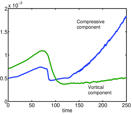
Figure 1: Quantitive evolution of compressive ($k_{com}=\sqrt{\sum_{k}|{\bf k}\cdot{\bf U}_{p}|^{2}/\sum_{k}|{\bf U}_{p}|^{2}}$) and vortical ($k_{vor}=\sqrt{\sum_{k}|{\bf k}\times{\bf U}_{p}|^{2}/\sum_{k}|{\bf U}_{p}|^{2}}$) components of plasma flow. Here ${\bf k}$ and $N_{k}$ are respectively the wave vector and total number of modes. The summation is carried over the entire turbulent spectrum. Initially, the vortical component is large. As time progresses, compressive component dominates over the vortical counter part in the heliosheath.

We now analyze statistics of magnetic field fluctuations in both compressive and non-compressive MHD plasma to describe the statistics of magnetic field fluctuations. It should be noted that the initial fluctuations in our simulations comprise both the vortical (i.e. irrotational motion of fluid flow) and compressional (due to the longitudinal flow motion) components. Our previous work show that the vortical component of fluid flow dominates over the compressive component in a supersonic solar wind plasma dastgeer2006 . We use this result as a basis to develop a self-consistent description of compressive plasma fluctuations. In the latter, the vortical motion is sustained predominantly by shear Alfvénic modes that govern nonlinear cascade in the solar wind plasma. The compressive modes, on the other hand, are composed of fast/slow modes. The former survives, whereas the latter decays in the solar wind dastgeer2006 . By contrast, the Voyager’s observations indicate that the solar wind becomes more compressive in the heliosheath plasma bur . Hence the compressive component of the flow is expected to dominate the vortical component in the heliosheath plasma. To understand this apparent discrepancy between the compressive and vortical modes in the solar wind and heliosheath plasmas, we follow the evolution of the two components in our simulations by initializing the velocity field with a higher magnitude of vortical component. Our simulation results are shown in Fig. (1) for $512^{2}$ modes in a two dimensional box of length $2\pi\times 2\pi$. The other parameters in our simulations are; charge exchange $k/k_{ce}\sim 0.1-0.01$, fixed time step $dt=10^{-3}$, and collision parameter $\nu\sim 0.1-0.001$. The background constant magnetic field $B_{0}=0.5$. Our simulations are fully nonlinear because the ratio of the mean and fluctuating magnetic fields $\delta{\bf B}/{\bf B}_{0}\sim 1$.

As the evolution proceeds, nonlinear interactions quench the vortical component and amplifies the compressive counterpart. Consequently, the latter grows, while the former decays eventually and stays constant. The compression of the velocity field corresponds essentially to the compression of the magnetic field by virtue of the field and flow that are coupled strongly under the ideal frozen-in-field state. Our multi fluid simulations thus demonstrate that progressive development of compressive turbulence plays a catalyzing role in the mode coversion (vortical to compressive) process. Once the mode conversion process is over, the two components decouple permanently and evolve independent of each other. Further growth of the compressive component in our simulation is ascribed to turbulent fluctuations that are converted predominantly into the compressive mode by nonlinear processes whereas minimal or almost no flux of energy is transmitted into the vortical motion. Our simulations results, describing the predominance of the compressive modes over the vortical as shown in Fig. (1), are qualitatively consistent with the Voyager’s observations bur .

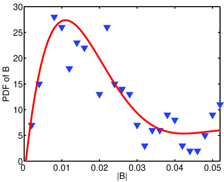
Figure 2: The magnetic field fluctuations in the non-compressive MHD turbulence exhibits a lognormal distribution in our simulations. The magnetic field fluctuations are dominated by the vortical modes.

IV statistics of magnetic field fluctuations

We next analyze the magnetic field fluctuations in our simulations. The results of our simulations, shown in Figs (2) & (3), describe probability distribution function (PDF) of the magnetic field fluctuations respectively in the non-compressive and compressive regimes of solar wind MHD turbulence. The PDF of the magnetic field in the non-compressive plasma is consistent with the lognormal distribution. This is shown in Fig. (2). By contrast, the magnetic field in the compressive plasma follows a Gaussian PDF as shown in Fig. (3). The latter is consistent with the Voyager 1 observations as reported by Burlaga et al. bur . A Gaussian PDF corresponds typically to a uniform, random and isotropic distribution, and a mean deviation in any of the latter leads essentially to a skewed or lognormal distribution Limpert . In the context of our simulations [see Figs (1) & (2)], we infer that a lognormal distribution of $B$ in the non-compressive plasma results primarily by the predominance of vortical motion in magnetized plasma that primarily gives rise to Alfvénic-like fluctuations. In the presence of a mean or background magnetic field, Alfvénic fluctuations tend to anisotropize the energy cascades kr ; sheb . Consequently, migration of turbulent energy is non symmetric along and across the mean magnetic field. The anisotropic cascade is therefore a process that could potentially lead to a skewed or lognormal distribution of the magnetic field in the non-compressive region which is dominated by nearly incompressible vortical motion. By contrast, plasma is dominated by the high frequency fluctuations in the compressed region. The effect of Alfvén waves is relatively weak in this region as compared to the vortically dominated non-compressive plasma. Owing thus to the weaker Alfvénic effect, the compressional and relatively high frequency motions in plasma tend to isotropize the magnetic field fluctuations. Hence a Gaussian PDF follows in the compressive plasma. The physical process, describing how Gaussian and lognormal distributions occur respectively in compressive and non-compressive plasma, is consistent with our simulations shown in Figs (1) & (2).

Figure 3: Probability distribution function of the magnetic field in the post-shock is consistent with the Gaussian distribution. The magnetic field fluctuations are dominated by the compressive modes.

V Conclusions

In summary, we have investigated evolution of the magnetic field fluctuations in small scale compressive and non-compressive MHD plasma turbulence in a partially ionized environment. Our results are useful in describing the magnetic field data from Voyagers bur . We find that initial turbulent fluctuations, comprising both the vortical and compressive motion, evolve towards a state in which the vortical motion predominantly governs nonlinear interaction in the non-compressive plasma by exciting Alfvénic modes. By contrast, the mode conversion process in the compressive plasma leads to the suppression of shear Alfvénic vortical modes whereas the compressive modes are amplified. The latter isotropizes the PDF of magnetic field in the compressive plasma.

To summarize our findings, we find that the probability distribution function of magnetic field in compressive MHD fluctuations is a Gaussian. The depleted vortical motions suppress the Alfvénic modes in the compressive MHD plasma. This we believe is one of the plaussible reasons why the magnetic field fluctuations are transformed into a Gaussian (from the lognormal) in partially ionized compressive solar wind plasma turbulence. Our results, consistent with the Voyager observations bur and theoretical predictions zank ; zank1996 , may be useful in the context of heliospheric plasma where charge exchange interactions govern numerous features of the solar wind plasma zank ; bur ; dastgeer .

References

- (1) P. K. Shukla, Physics Letters, vol. 60A, p. 223, 224, 1977.
- (2) P. K. Shukla, Nature, 274, 874, 1978.
- (3) E. Bengt, and P. K. Shukla, AIP Conf. Proc. – October 15, 2008 – Volume 1061, pp. 76-83 FRONTIERS IN MODERN PLASMA PHYSICS: ICTP International Workshop on the Frontiers of Modern Plasma Physics; DOI:10.1063/1.3013785
- (4) G. P. Zank, Sp. Sci. Rev., 89, 413-688, 1999.
- (5) G. P. Zank, and H. L. Pauls, Sp. Sci. Rev., 78, 95. 1996.
- (6) L. F. Burlaga, et al, ApJ, 642, 584, 2006.
- (7) D. Shaikh & G. P. Zank, ApJ 688, 683, 2008.
- (8) D. Shaikh & G. P. Zank, ApJ 640, L195, 2006.
- (9) E. Limpert, A. Stahel, and M. Abbt, BioScience, 51, 5, 341, 2001.
- (10) J. V. Shebalin, W. H. Matthaeus, and D. Montgomery, J. Plasma Physics 3, 525, 1983.
- (11) R. H. Kraichnan, Phys. Fluids, 8, 1385, 1965.