Variational inequality method in stock loans

Abstract.

In this paper we first introduce two new financial products: stock loan and capped stock loan. Then we develop a pure variational inequality method to establish explicitly the values of these stock loans. Finally, we work out ranges of fair values of parameters associated with the loans. MSC(2000): Primary 91B02, 91B70, 91B24; Secondary 60H10,91B28. Keywords: Capped stock loan, variational inequality method, perpetual American option, generalized Itô formula , Black-Scholes model.

1. Introduction

Stock loan is a simple economy where a client(borrower), who owns one share of a stock, borrows a loan of amount $q$ from a bank (lender) with one share of stock as collateral. The bank charges amount $c(0\leq c\leq q)$ from the client for the service. The client may regain the stock by repaying principal and interest (that is, $qe^{\gamma t}$, here $\gamma$ is continuously compounding loan interest rate ) to the bank, or surrender the stock instead of repaying the loan at any time. It is a currently popular financial product. It can create liquidity while overcoming the barrier of large block sales, such as triggering tax events or control restrictions on sales of stocks. It also can serve as a hedge against a market down: if the stock price goes down, the client may forfeit the loan at initial time; if the stock price goes up, the client keeps all the upside by repaying the principal and interest. Therefore, the stock loan has unlimited liability. As a result, stock loan transforms risk into the bank. To reduce the risk, the bank introduces cap $L$ feature in the stock loan because the cap adds a further incentive to exercise early. Such a loan is called a capped stock loan throughout this paper. Since the capped stock loan has limited liability and lower risk, it therefore will be an attractive instrument to market for an issuer, or to hold short for an investor like American call option with cap in financial market(cf. Broadie and Detemple [2](1995)). The wide acceptance and popular feature of the capped (uncapped) stock loan in the marketplace, however, greatly depend on how to make successfully these kinds of financial products. More precisely, how to work out right values of the parameters $(q,\gamma,c,L)$ is a natural and key problem in negotiation between the client and the bank at initial time. Unfortunately, to the authors’ best knowledge, it seems that few results on the topic have been reported in existing literature. The main goal of the present paper is to develop a pure variational inequality method to solve this kind of problems. We explain major difficulty and main idea of solving the problem as follows. We formulate the capped (uncapped) stock loan as a perpetual American option with negative interest rate. We denote by $f(x)$ the initial value of this option. The problem can be reduced to calculating the function $f(x)$ for determining the ranges of fair values of the parameters $(q,\gamma,c,L)$. According to the conventional variational inequality method, the $f(x)$ must satisfy a variational inequality, we calculate $f(x)$ by initial condition $f(0)=0$ and smooth-fit principle. However, because of negative interest rate the initial condition $f(0)=0$ does not work, i.e., the conventional variational inequality method can not solve this option with negative interest rate. Moreover, the presence of the cap also complicates the valuation procedure(if we focus on studying the capped stock loan). So we need to develop the variational inequality method to deal with the case of negative interest rate. As payoff process of the capped (uncapped) stock loan is a Markov process, the optimal stopping time must be a hitting time( Remark 3.1 below) from which we guess that $f^{\prime}(0)=0$. In addition, we observe that the condition do work in the case of negative interest rate but it has no use to dealing with the case of non-negative interest rate. Based on the conjecture and observation, we first establish explicitly the value $f(x)$ of the capped stock loan by a new pure variational inequality method. Then we use the expression of $f(x)$ to work out the ranges of fair values of parameters associated with the loan. Finally, as a special case of our main result, we also get the same conclusion on uncapped stock loan as in Xia and Zhou [13] proved by a pure probability approach. The paper is organized as follows: In Section 2, we formulate a mathematical model of capped stock loan and it is considered as a perpetual American option with a possibly negative interest rate. In Section 3, we extend standard variational inequality method to the case of negative interest rate and calculate the initial value and the value process of the capped(uncapped) stock loan. In Section 4, we work out the ranges of fair values of parameters associated with the loan based on the results in previous sections. In Section 5, we present two examples to explain how the cap impacts on the initial value of uncapped stock loan.

2. Mathematical model

In this section the standard Black-Scholes model in a continuous financial market consists of two assets: a risky asset stock $S$ and a risk-less bond $B$. The uncertainty is described by a standard Brownian motion $\{\mathbf{W}_{t},t\geq 0\}$ on a risk-neutral complete probability space $(\Omega,\mathcal{F},\{\mathcal{F}_{t}\}_{t\geq 0},P)$, where $\{\mathcal{F}_{t}\}_{t\geq 0}$ is the filtration generated by $\mathbf{W}$, $\mathcal{F}_{0}=\sigma\{\Omega,\emptyset\}$ and $\mathcal{F}=\sigma\{\bigcup_{t\geq 0}\mathcal{F}_{t}\}$. The risk-less bond $B$ evolves according to the following dynamic system,

$$dB_{t}=rB_{t}dt,\ \ r>0,$$

where $r$ is continuously compounding interest rate. The stock price $S$ follows a geometric Brownian motion,

$$S_{t}=S_{0}e^{(r-\delta-\frac{\sigma^{2}}{2})t+\sigma\mathbf{W}_{t}},$$ (2.1)

where $S_{0}$ is initial stock price, $\delta\geq 0$ is dividend yield and $\sigma>0$ is volatility. The discounted payoff process of the capped stock loan is defined by

$$Y(t)=e^{-rt}(S_{t}\wedge Le^{\gamma t}-qe^{\gamma t})_{+}.$$

Since $Y(t)\geq 0,\ a.s.$ and $Y(t)>0$ with a positive probability, to avoid arbitrage, throughout this paper we assume that

$$S_{0}-q+c>0.$$ (2.2)

According to theory of American contingent claim, the initial value of this capped stock loan is

$$f(x) = \sup\limits_{\tau\in\mathcal{T}_{0}}{\bf E}\big{[}e^{-r\tau}(S_{\tau}\wedge Le^{\gamma\tau}-qe^{\gamma\tau})_{+}\big{]}$$ (2.3)

$$= \sup\limits_{\tau\in\mathcal{T}_{0}}{\bf E}\big{[}e^{-\tilde{r}\tau}(\tilde{S}_{\tau}\wedge L-q)_{+}\big{]},$$

where $\tilde{r}=r-\gamma$, $\tilde{S}_{t}=e^{-\gamma t}S_{t},\tilde{S}_{0}=S_{0}=x$, $L>S_{0}$ and $\mathcal{T}_{0}$ denotes all $\{\mathcal{F}_{t}\}_{t\geq 0}$-stopping times. The value process of this capped stock loan is

$$V_{t}=\sup\limits_{\tau\in\mathcal{T}_{t}}{\bf E}\big{[}e^{-{r}(\tau-t)}(S_{\tau}\wedge Le^{\gamma\tau}-qe^{\gamma\tau})_{+}|\mathcal{F}_{t}\big{]},$$ (2.4)

i.e.,

$$e^{-rt}V_{t}=\sup\limits_{\tau\in\mathcal{T}_{t}}{\bf E}\big{[}e^{-\tilde{r}\tau}(\tilde{S}_{\tau}\wedge L-q)_{+}|\mathcal{F}_{t}\big{]},$$

where $\mathcal{T}_{t}$ denotes all $\{\mathcal{F}_{t}\}_{t\geq 0}$-stopping times $\tau$ with $\tau\geq t$ a.s.. Since the fair values of $q,\gamma,c,L$ should be such that $f(S_{0})=S_{0}-q+c$, the range of the fair values of the parameters $(q,\gamma,c,L)$ reduce to calculating the $f(S_{0})$. Because $\tilde{r}=r-\gamma\leq 0$, the problem is essentially to calculate the initial value of a conventional perpetual American call option with a possibly negative interest rate. We have the following.

Proposition 2.1.

$(x-q)_{+}\leq f(x)\leq x$ for $x\geq 0$. $f(x)$ is continuous and nondecreasing on $(0,\infty)$

Proof.

Using the same way as in Xia and Zhou [13](2007), we have $(x\wedge L-q)_{+}\leq f(x)\leq x\wedge L$ for $x\geq 0$. The $f(x)$ is continuous and nondecreasing on $(0,\infty)$ can be proved by the optional sampling theorem. ∎

3. Variational inequality method in stock loans

In this section we develop a pure variational inequality method in the case of negative interest rate to establish explicitly the value $f(x)$ of the capped (uncapped) stock loan. The key point is to replace the initial condition $f(0)=0$ in the conventional case with a new one $f^{\prime}(0+)=0$. The detailed observation will be given in Remark 3.1 below. We find that the condition $f^{\prime}(0+)=0$ holds for the conventional perpetual American call option but no use in determining free constants. Now we star with the following.

Proposition 3.1.

Assume that $\delta>0$ and $\gamma-r+\delta\geq 0$ or $\delta=0$ and $\gamma-r>\frac{\sigma^{2}}{2}$. Let $\lambda_{1}$, $\lambda_{2}$ and $\mu$ be defined by

$$\left\{\begin{array}[]{l l l}\lambda_{1}=\frac{-\mu+\sqrt{\mu^{2}-2(\gamma-r)}}{\sigma},\ \lambda_{2}=\frac{-\mu-\sqrt{\mu^{2}-2(\gamma-r)}}{\sigma},\\ \mu=-(\frac{\sigma}{2}+\frac{\gamma-r+\delta}{\sigma}).\end{array}\right.$$ (3.3)

(i)If $L\geq b$, $h(x)\in\mathcal{C}\big{(}[0,\infty)\big{)}\cap\mathcal{C}^{1}\big{(}(0,\infty)\setminus\{L\}\big{)}\cap\mathcal{C}^{2}\big{(}(0,\infty)\setminus\{b,L\}\big{)}$ and solves the variational inequality

$$\left\{\begin{array}[]{l l l l l}\frac{1}{2}\sigma^{2}x^{2}h^{{}^{\prime\prime}}+(\tilde{r}-\delta)xh^{{}^{\prime}}-\tilde{r}h=0,&x\in[0,b)\cup(L,\infty),\\ h(x)=x-q,&x\in[b,L],\\ h(x)>(x-q)_{+},&x<b,\\ h(x)\leq x,&x\geq 0,\\ h^{\prime}(0+)=0,\ h(b)=b-q,h^{{}^{\prime}}(b)=1,\end{array}\right.$$ (3.9)

then

$$h(x)=\left\{\begin{array}[]{l l l}(b-q)(\frac{x}{b})^{\lambda_{1}},&0<x\leq b,\\ x-q,&b<x<L,\\ (L-q)(\frac{x}{L})^{\lambda_{2}},&x\geq L.\end{array}\right.$$ (3.13)

Moreover,

$$b=\frac{q\lambda_{1}}{\lambda_{1}-1}.$$ (3.14)

(ii) If $L<b$, $h(x)\in\mathcal{C}\big{(}[0,\infty)\big{)}\cap\mathcal{C}^{1}\big{(}(0,\infty)\setminus\{L\}\big{)}\cap\mathcal{C}^{2}\big{(}(0,\infty)\setminus\{L\}\big{)}$ and solves the variational inequality

$$\left\{\begin{array}[]{l l l l}\frac{1}{2}\sigma^{2}x^{2}h^{{}^{\prime\prime}}+(\tilde{r}-\delta)xh^{{}^{\prime}}-\tilde{r}h=0,&x\in[0,L)\cup(L,\infty),\\ h(x)>(x-q)_{+},&x<L,\\ h(x)\leq x,&x\geq 0,\\ h^{\prime}(0+)=0,h(L)=L-q,\end{array}\right.$$ (3.19)

then

$$h(x)=\left\{\begin{array}[]{l l l}(L-q)(\frac{x}{L})^{\lambda_{1}},&0<x<L,\\ L-q,&x=L,\\ (L-q)(\frac{x}{L})^{\lambda_{2}},&x>L.\end{array}\right.$$ (3.23)

Proof.

We only deal with the part (i). The part (ii) can be treated similarly. Solving the first second-order differential equation of the(3.9), we get

$$h(x)=\left\{\begin{array}[]{l l l}C_{1}x^{\lambda_{1}}+C_{2}x^{\lambda_{2}},&x\in[0,b),\\ x-q,&x\in[b,L],\\ C_{3}x^{\lambda_{1}}+C_{4}x^{\lambda_{2}},&x\in(L,\infty),\end{array}\right.$$ (3.27)

where $C_{i}$, $i=1,2,3,4$, and $b$ are free constants to be determined, $\lambda_{1}$ and $\lambda_{2}$ are defined by (3.3). Note that if $\delta>0$ then $\lambda_{1}>1>\lambda_{2}>0$, and if $\delta=0$ and $\gamma-r>\frac{\sigma^{2}}{2}$ then $\lambda_{1}=\frac{2(\gamma-r)}{\sigma^{2}}>1=\lambda_{2}$. Using $h^{\prime}(0+)=0$ and $h(x)<x$, we have $C_{2}=C_{3}=0$. Substituting $C_{2}=C_{3}=0$ into (3.27) and applying $h(b)=b-q$, $h^{\prime}(b)=1$ as well as the principle of smooth fit in the resulting expression of $h(x)$ yields that

$$b-q=C_{1}b^{\lambda_{1}},\quad L-q=C_{4}L^{\lambda_{2}},\quad\lambda_{1}C_{1}b^{\lambda_{1}-1}=1.$$

Solving this system for $b$, $C_{1}$ and $C_{4}$, we get $b=\frac{q\lambda_{1}}{\lambda_{1}-1}$, $C_{1}=\frac{b-q}{b^{\lambda_{1}}}$ and $C_{4}=\frac{L-q}{L^{\lambda_{2}}}$. Hence the equations (3.13) and (3.14) follow. Since $\lambda_{1}>1\geq\lambda_{2}>0$ , the function $h(x)$ defined by (3.13) obviously belongs to $\mathcal{C}\big{(}[0,\infty)\big{)}\cap\mathcal{C}^{1}\big{(}(0,\infty)\setminus\{L\}\big{)}\cap\mathcal{C}^{2}\big{(}(0,\infty)\setminus\{b,L\}\big{)}.$ Thus we complete the proof. ∎

Remark 3.1.

From (3.3) we know that if $\widetilde{r}=r-\gamma>0$( the conventional case ) then $\lambda_{1}\geq 1>0$ and $\lambda_{2}<0$. Consequently, we see from (3.27) that the function $h(x)=C_{2}x^{\lambda_{2}}$ is rejected by the initial condition $h(0)=0$, i.e., $C_{2}=0$. So by the same way as in proof of Proposition 3.1 above, we can determine other free constants $C_{1}$, $C_{3}$, $C_{4}$ and $b$. If $\widetilde{r}=r-\gamma\leq 0$( the present case ) then $\lambda_{1}>1\geq\lambda_{2}>0$. As opposed to the conventional case, we can not deduce from $h(0)=0$ that $C_{2}=0$. This is the major difficulty appearing in variational inequality method in the case of stock loan. However, we note that in present case $h^{\prime}(x)=\lambda_{1}C_{1}x^{\widetilde{\lambda_{1}}}+\lambda_{2}C_{2}x^{\widetilde{\lambda_{2}}}$ with $\widetilde{\lambda_{1}}=\lambda_{1}-1>0$ and $\widetilde{\lambda_{2}}=\lambda_{2}-1<0$. So if $h^{\prime}(0+)=0$, the present case can be reduced to the conventional case. On the other hand, Markov property implies that the optimal stopping time must be a hitting time. In view of the fact, we conjecture that $h^{\prime}(0+)=0$ is correct. The proof of the conjecture will be given in Proposition 3.2 below. Comparing with the conventional case, the $h^{\prime}(0+)=0$ will play an important role in developing pure variational inequality method in the case of stock loan.

Proposition 3.2.

Assume that $\delta=0$, $\gamma-r>\frac{\sigma^{2}}{2}$ and $g(x)={\bf E}\big{[}e^{-\tilde{r}(\tau\wedge\varsigma)}(\tilde{S}_{\tau\wedge\varsigma}-q)_{+}I_{\{\varsigma<\infty\}}\big{]}$ for $b\geq q$, $L\geq 0$, stoping times $\tau$ and $\varsigma$. Then $g^{\prime}(0+)=0$.

Proof.

Using $g(0)=0$, we have for $x>0$

$$0 \leq \frac{g(x)-g(0)}{x-0}$$ (3.28)

$$= {\bf E}\large\{\large(\exp\{-\frac{1}{2}\sigma^{2}\tau\wedge\varsigma+\sigma\mathbf{W}_{\tau\wedge\varsigma}\}$$

$$\qquad-\frac{q}{x}\exp\{(\gamma-r)\tau\wedge\varsigma\}\large)_{+}I_{\{\varsigma<+\infty\}}\large\}$$

$$\leq {\bf E}\large\{\large(\exp\{-\frac{1}{2}\sigma^{2}\tau\wedge\varsigma+\sigma\mathbf{W}_{\tau\wedge\varsigma}\}-\frac{q}{x}\large)_{+}I_{\{\varsigma<+\infty\}}\large\}.$$

Note that $\large\{\exp\{-\frac{1}{2}\sigma^{2}t+\sigma\mathbf{W}_{t}\},t\geq 0\large\}$ is a strong martingale w.r.t. $\{\mathcal{F}_{t}\}_{t\geq 0}$. It follows that

$${\bf E}\large\{\exp\{-\frac{1}{2}\sigma^{2}\tau\wedge\varsigma+\sigma\mathbf{W}_{\tau\wedge\varsigma}\}\large\}=1.$$ (3.29)

To let $x\rightarrow 0$ in (3.28), we need to dominate the right-hand side. Because

$$\Large(\exp\{-\frac{1}{2}\sigma^{2}\tau\wedge\varsigma+\sigma\mathbf{W}_{\tau\wedge\varsigma}\}-\frac{q}{x}\Large)_{+}I_{\{\varsigma<+\infty\}}\leq\exp\{-\frac{1}{2}\sigma^{2}\tau\wedge\varsigma+\sigma\mathbf{W}{\tau\wedge\varsigma}\},$$

$$\lim_{x\rightarrow 0+}\Large(\exp\{-\frac{1}{2}\sigma^{2}\tau\wedge\varsigma+\sigma\mathbf{W}_{\tau\wedge\varsigma}\}-\frac{q}{x}\Large)_{+}I_{\{\varsigma<+\infty\}}=0.\quad a.s.,$$

and (3.29), the dominated convergence theorem allows us to let $x\rightarrow 0$ in (3.28) and obtain

$$0\leq\lim_{x\rightarrow 0+}\frac{g(x)-g(0)}{x-0}\leq\lim_{x\rightarrow 0+}{\bf E}\large\{\big{(}\exp\{-\frac{1}{2}\sigma^{2}\tau\wedge\varsigma+\sigma\mathbf{W}_{\tau\wedge\varsigma}\}-\frac{q}{x}\big{)}_{+}I_{\{\varsigma<+\infty\}}\large\}=0.$$

Thus $g^{{}^{\prime}}(0+)=0$. ∎

In view of Proposition 3.1 and variational inequality method, $\tau_{b}$ must be the optimal time, where $b$ is defined by (3.14). Now we show the fact.

Proposition 3.3.

Let $b$ and $h(x)$ be defined by (3.14), (3.13) and (3.23 ) respectively, $E(x)\equiv{\bf E}\big{[}e^{-\tilde{r}(\tau_{b}\wedge\tau_{L})}(\tilde{S}_{\tau_{b}\wedge\tau_{L}}\wedge L-q)_{+}I_{\{\tau_{L}<\infty\}}\big{]}$ for $L\geq 0$, where $x=S_{0}$, $\tau_{b}=\inf{\{t\geq 0:e^{-\gamma t}S_{t}\geq b\}}$ and $\tau_{L}=\inf{\{t\geq 0:e^{-\gamma t}S_{t}=L\}}$. Then $E(x)=h(x)$.

Proof.

Using formula 2.20.3 in Section 9, Part II of [1](2000), we have

$${\bf E}\big{[}e^{-\tilde{r}(\tau_{b}\wedge\tau_{L})}I_{\{\tau_{b}\wedge\tau_{L}<\infty\}}\big{]}=\left\{\begin{array}[]{l l}(\frac{x}{b})^{\lambda_{1}},x<b,\\ (\frac{x}{L})^{\lambda_{2}},x\geq L.\end{array}\right.$$ (3.32)

Based on the (3.32), the proof of Proposition 3.3 will be accomplished in two cases, namely, $L>b$ and $L\leq b$. Case of $L>b$. We shall distinguish three subcases, i.e., $x<b$, $L\geq x\geq b$ and $x\geq L$. If $x<b$ then $\tau_{b}\leq\tau_{L}$. Using(3.32), we calculate

$$E(x) = {\bf E}\big{[}e^{-\tilde{r}(\tau_{b}\wedge\tau_{L})}(\tilde{S}_{\tau_{b}\wedge\tau_{L}}\wedge L-q)_{+}I_{\{\tau_{L}<\infty\}}\big{]}$$ (3.33)

$$= {\bf E}\big{[}e^{-\tilde{r}(\tau_{b}\wedge\tau_{L})}(\tilde{S}_{\tau_{b}}\wedge L-q)_{+}I_{\{\tau_{L}<\infty\}}\big{]}$$

$$= (b-q)(\frac{x}{b})^{\lambda_{1}}.$$

If $L\geq x\geq b$ then $\tau_{b}=0$ and so

$$E(x) = {\bf E}\big{[}e^{-\tilde{r}(\tau_{b}\wedge\tau_{L})}(\tilde{S}_{\tau_{b}\wedge\tau_{L}}\wedge L-q)_{+}I_{\{\tau_{L}<\infty\}}\big{]}$$ (3.34)

$$= {\bf E}\big{[}(\tilde{S}_{0}\wedge L-q)_{+}\big{]}=(x-q).$$

If $x>L$ then $\tilde{S}_{\tau_{b}\wedge\tau_{L}}\geq L$. By using (3.32),

$$E(x) = {\bf E}\big{[}e^{-\tilde{r}(\tau_{b}\wedge\tau_{L})}(\tilde{S}_{\tau_{b}\wedge\tau_{L}}\wedge L-q)_{+}I_{\{\tau_{L}<\infty\}}\big{]}$$ (3.35)

$$= (L-q){\bf E}\big{[}e^{-\tilde{r}(\tau_{b}\wedge\tau_{L})}I_{\{\tau_{L}<\infty\}}\big{]}$$

$$= (L-q)(\frac{x}{L})^{\lambda_{2}}.$$

Comparing with (3.13), the equations (3.33), (3.34) and (3.35) yield that $E(x)=h(x)$. Case of $b\geq L$. We shall distinguish two subcases, i.e.,$x<L$ and $x\geq L$. If $x<L$ then $\tau_{b}\geq\tau_{l}$ . Using (3.32), we have

$$E(x) = {\bf E}\big{[}e^{-\tilde{r}(\tau_{b}\wedge\tau_{L})}(\tilde{S}_{\tau_{b}\wedge\tau{L}}\wedge L-q)_{+}I_{\{\tau_{L}<\infty\}}\big{]}$$ (3.36)

$$= {\bf E}\big{[}e^{-\tilde{r}(\tau_{b}\wedge\tau_{L})}(\tilde{S}_{\tau{L}}\wedge L-q)_{+}I_{\{\tau_{L}<\infty\}}\big{]}$$

$$= (L-q)(\frac{x}{L})^{\lambda_{1}}.$$

If $x\geq L$ then $\tilde{S}_{\tau_{b}\wedge\tau_{L}}\wedge L=L$. So by using (3.32)

$$E(x) = {\bf E}\big{[}e^{-\tilde{r}(\tau_{b}\wedge\tau_{L})}(\tilde{S}_{\tau_{b}\wedge\tau_{L}}\wedge L-q)_{+}I_{\{\tau_{L}<\infty\}}\big{]}$$ (3.37)

$$= (L-q){\bf E}\big{[}e^{-\tilde{r}(\tau_{b}\wedge\tau_{L})}I_{\{\tau_{L}<\infty\}}\big{]}$$

$$= (L-q)(\frac{x}{L})^{\lambda_{2}}.$$

Comparing the equations (3.36) and (3.37) with the (3.23), we see that $E(x)=h(x)$. ∎

We now return to main result of this section. It states that the initial value of the capped stock loan is just $f(x)$ defined by (3.13) and (3.23) respectively, where $x=S_{0}$.

Theorem 3.1.

Assume that $\delta>0$ and $\gamma-r+\delta\geq 0$ or $\delta=0$ and $\gamma-r>\frac{\sigma^{2}}{2}$. Let $h(x)$ be defined by (3.13) and (3.23)respectively, and $f(x)$ be defined by (2.3). Then $f(x)=h(x)$ for $x\geq 0$, and $\tau_{b}\wedge\tau_{L}$ is the optimal stopping time.

Proof.

In view of Proposition 3.3,

$$f(x)\equiv\sup\limits_{\tau\in\mathcal{T}_{0}}{\bf E}\big{[}e^{-\tilde{r}\tau}(\tilde{S}_{\tau}\wedge L-q)_{+}I_{\{\tau_{L}<\infty\}}\big{]}\geq h(x).$$

Therefore we only need to prove that for any stopping time $\tau$

$$h(x)\geq{\bf E}\big{[}e^{-\tilde{r}(\tau\wedge\tau_{L})}(\tilde{S}_{\tau\wedge\tau_{L}}\wedge L-q)_{+}I_{\{\tau_{L}<\infty\}}\big{]}.$$ (3.38)

From Proposition 3.1 and the expression of $h(x)$ as well as $\lambda_{1}>1\geq\lambda_{2}>0$, we know that $h(x)\in\mathcal{C}\big{(}[0,\infty)\big{)}\cap\mathcal{C}^{1}\big{(}(0,\infty)\setminus\{L\}\big{)}\cap\mathcal{C}^{2}\big{(}(0,\infty)\setminus\{b,L\}\big{)}$ or $h(x)\in\mathcal{C}\big{(}[0,\infty)\big{)}\cap\mathcal{C}^{1}\big{(}(0,\infty)\setminus\{L\}\big{)}\cap\mathcal{C}^{2}\big{(}(0,\infty)\setminus\{L\}\big{)}$ and $0<h^{\prime\prime}(b\pm)<+\infty$, $0<h^{\prime}(L\pm)<+\infty$ and $0<h^{\prime\prime}(L\pm)<+\infty$. As a result, the generalized Itô’s formula(cf.Karatzas and Shreve[5](1991) for Problem 6.24, p.215 ), the inequalities (3.9) and (3.19) yield

$$\int_{0}^{t}d(e^{-\tilde{r}s}h(\tilde{S}_{s})) = \int_{0}^{t}e^{-\tilde{r}s}\tilde{S}_{s}h^{{}^{\prime}}(\tilde{S}_{s})\sigma d\mathcal{W}(s)$$ (3.39)

$$+\int_{0}^{t}e^{-\tilde{r}s}(\tilde{r}q-\delta\tilde{S}_{s})I_{\{L>\tilde{S}_{s}\geq b^{*}\}}ds$$

$$+[h^{{}^{\prime}}(L+)-h^{{}^{\prime}}(L-)]\int_{0}^{t}e^{-\tilde{r}s}dL_{s}(L)$$

$$\equiv \mathcal{M}(t)+A_{1}(t)+\Lambda(t),$$

where $L_{t}(L)\geq 0$ is the local time of $\tilde{S}_{t}$ at the point $L$, $\mathcal{M}(t)=\int_{0}^{t}e^{-\tilde{r}s}\tilde{S}_{s}h^{{}^{\prime}}(\tilde{S}_{s})\sigma d\mathcal{W}(s)$ is a martingale,

$$A_{1}(t) = \int_{0}^{t}e^{-\tilde{r}s}(\tilde{r}q-\delta\tilde{S}_{s})I_{\{L>\tilde{S}_{s}\geq b^{*}\}}ds\qquad\mbox{and}$$

$$\Lambda(t) = \ \ [h^{{}^{\prime}}(L+)-h^{{}^{\prime}}(L-)]\int_{0}^{t}e^{-\tilde{r}s}dL_{s}(L).$$

Define $T_{n}=t\wedge\tau\wedge\tau_{L}-\frac{1}{n}$ for $\forall t\geq 0$ , $n\geq 1$ and stopping time $\tau$. Then by using definition of $\tau_{L}$ and equality $L_{t}(L)=\int^{t}_{0}I_{\{s:\tilde{S}_{s}=L\}}dL_{s}(L)$, we have $\Lambda(T_{n})=0$. Moreover, since $\tilde{r}\leq 0$ and $\delta\geq 0$, we see that $A_{1}(T_{n})\leq 0$. So by (3.39)

$$h(\tilde{S}_{0}) = {\bf E}\big{[}e^{-\tilde{r}T_{n}}h(\tilde{S}_{T_{n}})I_{\{\tau_{L}<\infty\}}\big{]}+{\bf E}\big{[}-A_{1}(T_{n})I_{\{\tau_{L}<\infty\}}\big{]}$$

$$\geq {\bf E}\big{[}e^{-\tilde{r}T_{n}}h(\tilde{S}_{T_{n}})I_{\{\tau_{L}<\infty\}}\big{]}$$

$$= {\bf E}\big{[}e^{-\tilde{r}T_{n}}h(\tilde{S}_{T_{n}})I_{\{\tau_{L}<\infty\}}\big{]}$$

$$\geq {\bf E}\big{[}e^{-\tilde{r}T_{n}}(\tilde{S}_{T_{n}}\wedge L-q)_{+}I_{\{\tau_{L}<\infty\}}\big{]}.$$

Note that

$$e^{-\tilde{r}T_{n}}(\tilde{S}_{T_{n}}\wedge L-q)_{+}I_{\{\tau_{L}<\infty\}}\leq\sup\limits_{0\leq t<\infty}e^{-\tilde{r}t}(\tilde{S}_{t}-q)_{+}$$

and

$${\bf E}\big{[}\sup\limits_{0\leq t<\infty}e^{-\tilde{r}t}(\tilde{S}_{t}-q)_{+}\big{]}<\infty.$$

The dominated convergence theorem now implies

$$h(x)=h(\tilde{S}_{0}) \geq \lim_{n\rightarrow+\infty}{\bf E}\big{[}e^{-\tilde{r}T_{n}}(\tilde{S}_{T_{n}}\wedge L-q)_{+}I_{\{\tau_{L}<\infty\}}\big{]}$$

$$= {\bf E}\big{[}e^{-\tilde{r}(\tau\wedge\tau_{L})}(\tilde{S}_{\tau\wedge\tau_{L}}\wedge L-q)_{+}I_{\{\tau_{L}<\infty\}}\big{]}.$$

Thus $h(x)=f(x)$ and $\tau_{b}\wedge\tau_{L}$ is the optimal stopping time. ∎

As a direct consequence of Theorem 3.1, i.e., $L=+\infty$, we can get the following result proved by a pure probability approach in Xia and Zhou[13].

Corollary 3.1.

Let $f(x)=\sup\limits_{\tau\in\mathcal{T}_{0}}{\bf E}\big{[}e^{-\tilde{r}\tau}(\tilde{S}_{\tau}-q)_{+}\big{]}$, $b$ and $\lambda_{1}$ be defined by (3.14) and (3.3) respectively. Then

$$f(x)=\left\{\begin{array}[]{l l l}(b-q)(\frac{x}{b})^{\lambda_{1}},&0<x\leq b,\\ x-q,&x>b\end{array}\right.$$ (3.42)

and $\tau_{b}$ is the optimal stoping time.

Remark 3.2.

Comparing with the value of capped American option with non-negative interest rate(cf.Broadie and Detemple [2](1995) ), we see that the value of capped stock loan treated in the present paper has different behaviors. If the stock price is bigger than $L$ then the capped American option with non-negative interest rate should be exercise immediately. While the capped stock loan treated in the present paper has no this kind of performances.

Remark 3.3.

Let $V_{t}$ be the value process for the capped stock loan defined by (2.4). Then by using Markov property of the process $S_{t}$ (cf. Karatzas and Shreve[6](1998)), we easily get

$$e^{-\tilde{r}t}f(\tilde{S}_{t}) = \sup\limits_{\tau\in\mathcal{T}_{t}}{\bf E}\big{[}e^{-\tilde{r}(\tau\wedge\tau_{L})}(\tilde{S}_{\tau\wedge\tau_{L}}\wedge L-q)_{+}I_{\{\tau_{L}<\infty\}}|\mathcal{F}_{t}\big{]}$$

$$= e^{-rt}V_{t}$$

and $V_{t}=e^{\gamma t}f(e^{-\gamma t}S_{t})$.

4. Ranges of fair values of parameters

In this section we will work out the ranges of fair values of the parameters $(q,\gamma,c,L)$ of the capped stock loan treated in this paper based on Theorem 3.1 and equality $f(S_{0})=S_{0}-q+c$. In view of Proposition3.1, there are two cases to be dealt with. The first is when $L>b$ and the second case is when $L\leq b$. We only consider the first case, the second case can be treated similarly. We shall distinguish three subcases, i.e., $S_{0}\geq L$, $L>S_{0}\geq b$ and $0<S_{0}\leq b$. Case of $S_{0}\geq L$. By (3.13) and $f(S_{0})=S_{0}-q+c$, we have $f(S_{0})=(L-q)(\frac{S_{0}}{L})^{\lambda_{2}}=S_{0}-q+c$. So the parameters $\gamma$, $q$, $c$ and $L$ must satisfy $c=(L-q)(\frac{S_{0}}{L})^{\lambda_{2}}+q-S_{0}\leq 0$. This means that the bank wants to earn maximal profit because the initial stock price is very high. The bank gets the stock via paying the money $c$ to the client, the client gives the stock to the bank due to the money $c$. Therefore both the client and the bank have incentives to do the business. Actually, $\tau_{L}$ is the optimal stopping time for the client to terminate the capped stock loans. Case of $L>S_{0}\geq b$. By (3.13) and $f(S_{0})=S_{0}-q+c$, we have $f(S_{0})=S_{0}-q=S_{0}-q+c$, so $c=0$, i.e., the client has no incentive to do the transaction. $\tau_{b}=0$ in this case is the optimal stopping time. Case of $0<S_{0}\leq b$. In this case both the client and the bank have incentives to do the business. The bank does because there is dividend payment and so does the client because the initial stock price is neither very high nor too low. By Theorem 3.1, the initial value is $f(S_{0})$. In this case the bank charges an amount $c=f(S_{0})-S_{0}+q$ from the client for providing the service. So the fair values of the parameters $\gamma,q$ and $c$ must satisfy

$$S_{0}-q+c=(b-q)(\frac{x}{b})^{\lambda_{1}}$$

and the optimal stopping time is $\tau_{b}$.

5. Examples

In this section we will give two examples of capped stock loan as follows.

Example 5.1.

Let the risk free rate $r=0.05$, the loan rate $\gamma=0.07$, the volatility $\sigma=0.15$, the dividend $\delta=0.01$, the principal $q=100$ and the cap $L=240$. Then $b=147.8<L$. We compute the initial value $f(x)$ of capped stock loan as in the following Figure 1. The graph obviously shows that the cap greatly impacts on the initial value when the stock price is very large. The cap reduces the value of the stock loan and the client can acquires more liquidity.

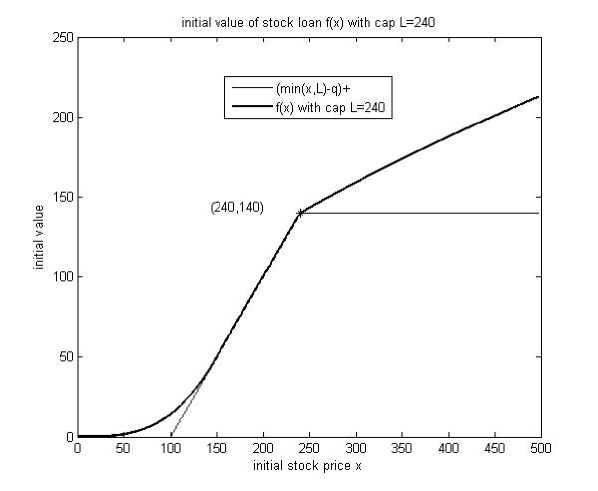
Figure 1. $\gamma=0.07,r=0.05,\sigma=0.15,\delta=0.01,q=100,cap=240$

Example 5.2.

Let $r$, $\sigma$, $\sigma$, $\delta$ and $q$ be as the same as in Example 5.1, $L=120$. Then $L<b=147.8$. We compute the initial value $f(x)$ of capped stock loan as in the following Figure 2. The graph explains that the initial value of caped stock loan greatly decreases because the cap is less than $b$. The client will acquire much more liquidity compared to the uncapped stock loan.

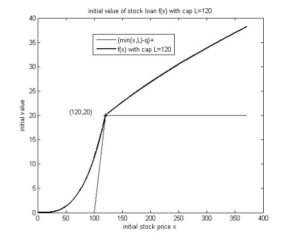
Figure 2. $\gamma=0.07,r=0.05,\sigma=0.15,\delta=0.01,q=100,cap=120$

Acknowledgements. We are very grateful to Professor Jianming Xia for his conversation with us and providing original paper of [13] for us. We also express our deep thanks to Professor Xun Yu Zhou for providing power point files of his talk on stock loan at Peking University for us. Special thanks also go to the participants of the seminar stochastic analysis and finance at Tsinghua University for their feedbacks and useful conversations. This work is supported by Project 10771114 of NSFC, Project 20060003001 of SRFDP, and SRF for ROCS, SEM, and the Korea Foundation for Advanced Studies. We would like to thank the institutions for the generous financial support.

References

- [1] Borodin, A. N., Salminen, P., 2002. Handbook of Brownian Motion-Facts and Formulae. Probability and its Applications, Birkhuser Verlag, Basel, 2nd edition.
- [2] Broadie, M., Detemple, J., 1995. American capped call options on dividend-paying asset . The Review of Finance Studies, Vol. 8, No. 1, pp. 161-191.
- [3] Dayanik, S., Karatzas, I., 2003. On the optimal stopping problems for one-dimensional diffusions. Stochastic Process. Appl., 107, no. 2, 173-212.
- [4] Jiang, S., Liang, Z., Wu, W., 2008. Stock loan with automatic termination clause. Preprint(11, 2008).
- [5] Karatzas, I., Shreve,S. E., 1991. Brownian motion and stochastic calculus. Springer-Verlag, New York.
- [6] Karatzas, I., Shreve,S. E., 1998. Methods of mathematical finance. Springer-Verlag, New York.
- [7] Kifer,Y., 2000. Game Options. Finance and Stochastics, 4:443-463.
- [8] Kyprianou, A.E., 2004. Some calculations for Israeli options. Finance and Stochastics, 8:73-86.
- [9] Lions, P.-L., Sznitman, A.S.. 1984. Stochastic differential equations with reflecting boundary conditions. Comm.Pure Appl. Math.37, 511-537.
- [10] McKean,H.P.JR., 1965. A free-boundary problem for the heat equation arising from a problem in mathematical economics. Industr. Manag. Rev., 6, 32-39. Appendix to Samuelson(1965a).
- [11] ksendal,B. and Sulem,A., 2005. Applied Stochastic Control of Jump Diffusions. Springer.
- [12] Shiryaev,A.N., Kabanov,Y.M., Kramkov, D.O. and Melnikov, A.V., 1994. Towards the theory of options of both European and American types II. Theory Prob.Appl, 39,61-102.
- [13] Xia, J.M., Zhou,X.Y., 2007. Stock loans. Mathematical Finance, Vol.17, No.2, 307-317.