Theoretical and numerical Analysis on Optimal dividend policy of an insurance company with positive transaction cost and higher solvency

Abstract.

Based on a point of view that solvency and security are first, this paper considers regular-singular stochastic optimal control problem of a large insurance company facing positive transaction cost asked by reinsurer under solvency constraint. The company controls proportional reinsurance and dividend pay-out policy to maximize the expected present value of the dividend pay-outs until the time of bankruptcy. The paper aims at deriving the optimal retention ratio, dividend payout level, explicit value function of the insurance company via stochastic analysis and PDE methods. The results present the best equilibrium point between maximization of dividend pay-outs and minimization of risks. The paper also gets a risk-based capital standard to ensure the capital requirement of can cover the total given risk. We present numerical results to make analysis how the model parameters, such as, volatility, premium rate, and risk level, impact on risk-based capital standard, optimal retention ratio, optimal dividend payout level and the company’s profit. MSC(2000): Primary 91B30,91B70,93E20; Secondary 60H30, 60H10. Keywords: Regular-singular stochastic optimal control; Stochastic differential equations; Positive transaction cost; Dividend payout level and retention ratio; Optimal return function; Solvency.

1. Introduction

In this paper we consider a problem of risk control and dividend optimization for a large insurance company facing positive transaction cost asked by reinsurer( that is, the case of excess-of-loss reinsurance). The company controls dividend stream and its risk, as well as potential profit by choosing different business activities among all of available policies to it. The objective of the insurer is to choose proportional reinsurance and dividend level to maximize the expected present value of the dividend pay-outs until the time of bankruptcy. This is a regular-singular control problem of diffusion processes. In the view of optimization of the dividend pay-outs, the stochastic optimal control problems of a large insurance company have been given attention by many authors recently. We refer the readers to Taksar and Zhou[24](1998), Choulli, Taksar and Zhou[5](2001), Højgaard and Taksar[11, 12](1999, 2001), Asmussen et all[2, 3](1997,2000), Guo, Liu and Zhou [7](2004), He and Liang[15, 17](2008) and other authors’ works. According to classical economic theory, the approach used in some of these papers is the insurer selects one from all admissible business arrangements to yield maximization of expected present value of dividend pay-outs. However, Although this ideal approach is the best in concept, it can’t be used in practice because the insurance business is a business affected with a public interest and consumers should be protected against insurer insolvencies (cf.Chapter 34, Williams and Heins[26](1985), Riegel and Miller [23](1963), Welson and Taylor [25](1958) ). Therefore, a policy making the company go bankrupt before termination of contract between insurer and policy holders or a policy of low solvency(where solvency means $1-$ probability of bankruptcy, cf.Bowers, Gerber et all [4](1997)) does not seem to be the best way and should be prohibited even though it has the highest gain because under which no claims will return to policy holders and contract can not be forced to perform. On the other hand, this policy will also worsen basis of insurance business survival and company’s reputation which is the company’s chief asset- a plant of long growth but peculiarly susceptible to the cold winds of idle rumor. So the higher standard of security and solvency is the first factor to be taken into account for insurer. Unfortunately, there are very few results concerning on stochastic optimal control problems of insurance company from a view of security and solvency are first. Paulsen [22](2003) first studied this kinds of optimal controls for diffusions via properties of return function and then He, Hou and Liang[16](2008) investigated the optimal control problems for linear Brownian model in case of cheaper reinsurance. By an innovative idea, based on a point of view that security and solvency are first, in this paper we will establish a sophisticated setting to effectively solve this kind of optimal control on problems of a large insurance company in case of positive transaction cost and solvency constraint. We aim at deriving the optimal retention ratio, dividend payout level, explicit value function of the insurance company via stochastic analysis and PDE methods. The model treated and approach used in the present paper are different from those of [22]. In our approach, only admissible policies satisfying this standard of security are considered, so it will reduce the insurer’s expected present value of dividend pay-outs, on the other hand, it will increase security and solvency in some sense by minimal loss. From this set of admissible policies, the insurer can select one that allows the highest expected present value of dividend pay-outs. Indeed, Our results present the best place between gains and risks, the loss for higher security and solvency is minimal. To get these results we first study some properties of probability of bankruptcy by stochastic analysis and PDE methods, then solve a generalized HJB equations in appendix , finally we prove that solution of the HJB is the optimal return function of the company. We find that the case treated in the [16](2008) is a trivial case, that is, the company of the model in the [16](2008) will never go to bankruptcy, it is an ideal model in concept, and it indeed does not exist in reality. Because probability of bankruptcy for the model treated in the present paper is very large, our results can not be directly deduced from the [16](2008). The paper is organized as follows. In next section we establish mathematical model of a large insurance company treated in this paper. In section 3 we present main result of this paper and its economic interpretations. In section 4 we analyze solvency and security of stochastic mathematical model considered in this paper, the results in this section also state that the solvency constraint set $\mathfrak{B}$ in section 3 is not empty set nor $R_{+}$, so the setting treated in this paper is well defined. In section 5 we present numerical results studying how the model parameters impact on the optimal return function and dividend policy. In section 6 we list some lemmas of properties of bankrupt probability, and their rigorous proofs are presented in section 8. We give detailed proofs of main results of this paper in section 7. Optimal return function and its robustness properties w.r.t. dividend level are given in appendix.

2. Mathematical model of a large insurance company

We start with a filtered probability space $(\Omega,\mathcal{F},\{\mathcal{F}_{t}\}_{t\geq 0},\mathbf{P})$ with a standard Brownian motion $\{W_{t}\}_{t\geq 0}$ on it, adapted to the filtration $\mathcal{F}_{t}$ satisfying the usual conditions. A pair of $\mathcal{F}_{t}$ adapted processes $\pi=\{a_{\pi}(t),L^{\pi}_{t}\}$ is called a admissible policy if $0\leq a_{\pi}(t)\leq 1$ and $L^{\pi}_{t}\$ is a nonnegative, non-decreasing, right-continuous with left limits. We denote by $\Pi$ the whole set of admissible policies. Given an admissible policy $\pi$, if we denote by $R^{\pi}_{t}$ the reserve of a large insurance company at time $t$ and by $L^{\pi}_{t}$ cumulative amount of dividends paid out to the shareholders up to time $t$, then, by using the center limit theorem, we can assume that (see [5, 24, 2, 6, 8, 9, 10]) the dynamics of $R^{\pi}_{t}$ is given by

$$dR^{\pi}_{t}=(\mu-(1-a_{\pi}(t))\lambda)dt+\sigma a_{\pi}(t)d{W}_{t}-dL^{\pi}_{t},\quad R^{\pi}_{0}=x,$$ (2.1)

where $1-a(t)$ is the reinsurance fraction at time $t$, the $R^{\pi}_{0}=x$ means that the initial liquid reserve is $x$, the constants $\mu$ and $\lambda$ can be regarded as the safety loadings of the insurer and reinsurer, respectively. Throughout this paper we assume that transaction cost $\lambda-\mu>0$. We refer readers to He, Hou and Liang[16](2008) for $\lambda=\mu$. When the reserve vanishes, we say that the company is bankrupt. We define the time of bankruptcy by $\tau^{\pi}_{x}=\inf\big{\{}t\geq 0:R^{\pi}_{t}=0\big{\}}$. Obviously, $\tau^{\pi}_{x}$ is an $\mathcal{F}_{t}$ -stopping time. For any $b\geq 0$, let $\Pi_{b}=\{\pi\in\Pi:\int_{0}^{\infty}I_{\{s:R^{\pi}(s)<b\}}dL_{s}^{\pi}=0\}$. It is easy to see that $\Pi=\Pi_{0}$ and $b_{1}>b_{2}\Rightarrow\Pi_{b_{1}}\subset\Pi_{b_{2}}$. For a given admissible policy $\pi$ we define value function $V(x)$ of a large insurance company by

$$J(x,\pi) = \mathbb{E}\big{\{}\int_{0}^{\tau^{\pi}_{x}}e^{-ct}dL_{t}^{\pi}\big{\}},$$

$$V(x,b) = \sup_{\pi\in\Pi_{b}}\{J(x,\pi)\},$$ (2.2)

$$V(x) = \sup_{b\in\mathfrak{B}}\{V(x,b)\}$$ (2.3)

where the solvency set $\mathfrak{B}$ defined by

$$\mathfrak{B}:=\big{\{}b\ :\ \mathbb{P}[\tau_{b}^{\pi_{b}}\leq T]\leq\varepsilon\ ,\ J(x,\pi_{b})=V(x,b)\mbox{ and}\ \pi_{b}\in\Pi_{b}\big{\}},$$

$c>0$ is a discount rate, $\tau_{b}^{\pi_{b}}$ is the time of bankruptcy $\tau_{x}^{\pi_{b}}$ when the initial asset $x=b$ and the control policy is $\pi_{b}$. $1-\varepsilon$ is the standard of security and less than solvency for given $\varepsilon>0$( see [21, 4]). The main purpose of this paper is to solve the optimal control problems (2) and (2.3). In addition to finding optimal return function $V(x)$ of the company, we also derive the optimal retention ratio, dividend payout level $b^{*}$ and optimal policy $\pi^{*}_{b^{*}}$ associated with the $V(x)$ such that $J(x,\pi^{*}_{b^{*}})=V(x)$. Moreover, their robustness properties w.r.t. model parameters are presented via numerical results.

3. Main Results

In this section we first present main results of this paper, then, together with numerical results in section 5 below, give economic and financial interpretations of the main results. The results present the best equilibrium point between benefits and risks. The proofs of main results will be given in section 7.

Theorem 3.1.

Assume that transaction cost $\lambda-\mu>0$. Let level of risk $\varepsilon\in(0,1)$ and time horizon $T$ be given. (i) If $\mathbf{P}[\tau_{b_{0}}^{\pi^{*}_{b_{0}}}\leq T]\leq\varepsilon$, then the value function $V(x)$ of the company is $f(x)$ defined by (9.8) and (9.14) in appendix, and $V(x)=V(x,b_{0})=J(x,\pi^{*}_{b_{0}})=V(x,0)=f(x)$. The optimal policy associated with $V(x)$ is $\pi_{b_{o}}^{\ast}=\{A^{*}_{b_{0}}(R^{\pi_{b_{o}}^{\ast}}_{\cdot}),L^{\pi_{b_{o}}^{\ast}}_{\cdot}\}$, where $(R^{\pi_{b_{0}}^{\ast}}_{t},L_{t}^{\pi_{b_{0}}^{\ast}})$ is uniquely determined by the following SDE with reflection boundary(cf.[20]):

$$\left\{\begin{array}[]{l l l}dR_{t}^{\pi_{b_{o}}^{\ast}}=(\mu-(1-A^{*}_{b_{0}}(R^{\pi_{b_{o}}^{\ast}}_{t}))\lambda)dt+\sigma A^{*}_{b_{0}}(R^{\pi_{b_{o}}^{\ast}}_{t})d{W}_{t}-dL_{t}^{\pi_{b_{o}}^{\ast}},\\ R_{0}^{\pi_{b_{o}}^{\ast}}=x,\\ 0\leq R^{\pi_{b_{o}}^{\ast}}_{t}\leq b_{0},\\ \int^{\infty}_{0}I_{\{t:R^{\pi_{b_{o}}^{\ast}}_{t}<b_{0}\}}(t)dL_{t}^{\pi_{b_{o}}^{\ast}}=0\end{array}\right.$$ (3.5)

and $\tau_{x}^{\pi^{*}_{b_{0}}}=\inf\{t:R^{\pi_{b_{0}}^{\ast}}_{t}=0\}$. The optimal dividend level is $b_{0}$(see Lemma A.1 ), where $A^{*}(x)$ is defined by part (iii) of Lemma A.1 in appendix. The solvency of the company is bigger than $1-\varepsilon$. (ii) If $\mathbf{P}[\tau_{b_{0}}^{\pi^{*}_{b_{0}}}\leq T]>\varepsilon$, then there is a unique $b^{*}>b_{0}$ satisfying $\mathbf{P}[\tau_{b^{*}}^{\pi^{*}_{b^{*}}}\leq T]=\varepsilon$ such that $g(x)$ defined by (9.28) and (9.32) in appendix is the value function of the company, that is,

$$g(x)=\sup_{b\in\mathfrak{B}}\{V(x,b)\}=V(x,b^{*})=J(x,\pi^{*}_{b^{*}})$$ (3.6)

and

$$b^{*}\in\mathfrak{B},$$ (3.7)

where

$$\mathfrak{B}:=\big{\{}b:\mathbb{P}[\tau_{b}^{\pi_{b}}\leq T]\leq\varepsilon,\ J(x,\pi_{b})=V(x,b)\mbox{ and}\ \pi_{b}\in\Pi_{b}\ \big{\}}.$$

The optimal policy associated with $g(x)$ is $\pi_{b^{*}}^{\ast}=\{A^{*}_{b^{*}}(R^{\pi_{b^{*}}^{\ast}}_{\cdot}),L^{\pi_{b^{*}}^{\ast}}_{\cdot}\}$, where $(R^{\pi_{b^{*}}^{\ast}}_{\cdot},L^{\pi_{b^{*}}^{\ast}}_{\cdot}\})$ is uniquely determined by the following SDE with reflection boundary:

$$\left\{\begin{array}[]{l l l}dR_{t}^{\pi_{b^{*}}^{\ast}}=(\mu-(1-A^{*}_{b^{*}}(R^{\pi_{b^{*}}^{\ast}}_{t}))\lambda)dt+\sigma A^{*}_{b^{*}}(R^{\pi_{b^{*}}^{\ast}}_{t})d{W}_{t}-dL_{t}^{\pi_{b^{*}}^{\ast}},\\ R_{0}^{\pi_{b^{*}}^{\ast}}=x,\\ 0\leq R^{\pi_{b^{*}}^{\ast}}_{t}\leq b^{*},\\ \int^{\infty}_{0}I_{\{t:R^{\pi_{b^{*}}^{\ast}}_{t}<b^{*}\}}(t)dL_{t}^{\pi_{b^{*}}^{\ast}}=0\end{array}\right.$$ (3.12)

and $\tau_{x}^{\pi^{*}_{b}}=\inf\{t:R^{\pi_{b}^{\ast}}_{t}=0\}$. The optimal dividend level is $b^{*}$, where $A^{*}_{b^{*}}(x)$ is defined by part (iii) of Lemma A.2 in appendix. The optimal dividend policy $\pi^{*}_{b^{*}}$ and the optimal dividend $b^{*}$ ensure that the solvency of the company is $1-\varepsilon$. (iii) Moreover,

$$\frac{g(x,b^{*})}{g(x,b_{0})}\leq 1.$$ (3.13)

We give economic and financial explanation of Theorem 3.1 is as follows: (1) For a given level of risk and time horizon, if probability of bankruptcy is less than the level of risk, the optimal control problem of (2) and (2.3) is the traditional one, the company has higher solvency, so it will have good reputation. The solvency constraints here do not work. (2) If probability of bankruptcy is large than the level of risk, the traditional optimal policy will not meet the standard of security and solvency, the company needs to find a sub-optimal policy $\pi_{b^{*}}^{\ast}$ to improve its solvency. The sub-optimal reserve process $R^{\pi_{b^{*}}^{\ast}}_{t}$ is a diffusion process reflected at $b^{*}$, the process $L^{\pi_{b^{*}}^{\ast}}_{t}$ is the process which ensures the reflection. The sub-optimal action is to pay out everything in excess of $b^{*}$ as dividend and pay no dividend when the reserve is below $b^{*}$, and $A^{*}_{b^{*}}$ is the sub-optimal feedback control function.(3) On the one hand, the inequality (3.13) states that $\pi_{b^{*}}^{\ast}$ will reduce the company’s profit, on the other hand, in the view of (3.13), $\mathbb{P}[\tau_{b^{\ast}}^{\pi_{b^{*}}^{\ast}}\leq T]=\varepsilon$ and Corollary A2 below, the cost of improving solvency is minimal. Therefore the policy $\pi_{b^{*}}^{\ast}$ is the best equilibrium action between making profit and improving solvency.(4) The under writing risk $\sigma^{2}$, the premium rate $\mu$ and the initial capital $x$ will increase the company’s return, see the graphs 1 and 2 in section 5 below. (5) The risk-based capital standard $x$ decreases with the preferred risk level $\varepsilon$, so the higher preferred risk level $\varepsilon$ only needs a lower initial risk-based capital, see the graph 4 below. (6) The optimal dividend level $b(\varepsilon)$ is a decreasing function of the risk level $\varepsilon$, by comparison theorem of SDE, the optimal retention ratio decreases with $\varepsilon$, but the optimal dividend process increases with $\varepsilon$. Inversely, the risk level $\varepsilon(b)$ is also a decreasing function of $b$ (see the graphs 5 and 6 below ).

Remark 3.1.

Because the [16] had no continuity of probability of bankruptcy and actual $b^{*}$, the authors of [16] did not obtain the best equilibrium policy $\pi_{b^{*}}^{\ast}$.

4. Analysis on the security and solvency of control model

In this section we will give a quantitative analysis about the security and solvency of stochastic control model treated in this paper. The main result of this section is Theorems 4.1 and 4.2 below. They reveal that for any given $T>0$ low dividend $b_{0}$ will raise level of risk $\varepsilon_{0}$, the company does have higher level of risk before the contract between insurer and policy holder goes into effect(i.e., $T$ is less than the time of the contract issue and positive), the company’s solvency is less than $1-\varepsilon_{0}$, so the company has to find an optimal dividend policy that improves the ability of the insurer to fulfill its obligation to policy holders under higher standard of security and solvency. On the other hand, the solvency constraint set $\mathfrak{B}$ in section 3 is not empty set nor $R_{+}$, the setting treated in this paper is well defined.

Theorem 4.1.

Assume that $\lambda>\mu$ and define process $(R^{\pi_{b_{0}}^{\ast},x}_{t},L^{\pi_{b_{0}}^{\ast}}_{t})$ by the following SDE:

$$\left\{\begin{array}[]{l l l}dR_{t}^{\pi_{b_{o}}^{\ast},x}=(\mu-(1-A^{*}_{b_{0}}(R^{\pi_{b_{o}}^{\ast},x}_{t}))\lambda)dt+\sigma A^{*}_{b_{0}}(R^{\pi_{b_{o}}^{\ast},x}_{t})d{W}_{t}-dL_{t}^{\pi_{b_{o}}^{\ast}},\\ R_{0}^{\pi_{b_{o}}^{\ast},x}=x,\\ 0\leq R^{\pi_{b_{o}}^{\ast},x}_{t}\leq b_{0},\\ \int^{\infty}_{0}I_{\{t:R^{\pi_{b_{o}}^{\ast},x}_{t}<b_{0}\}}(t)dL_{t}^{\pi_{b_{o}}^{\ast}}=0.\end{array}\right.$$ (4.5)

Then for any $0<x\leq b_{0}$ there exists $\varepsilon_{0}>0$ such that

$$\mathbf{P}\{\tau_{x}^{\pi_{b_{0}}^{\ast}}\leq T\}\geq\varepsilon_{0}>0,$$ (4.6)

where $\varepsilon_{0}=\min\big{\{}\frac{4[1-\Phi(\frac{x}{d\sigma\sqrt{T}})]^{2}}{\exp\{\frac{2}{\sigma^{2}}(\lambda^{2}+\delta^{2})T\}},\frac{x}{\sqrt{2\pi}\sigma}\int^{T}_{0}t^{-\frac{3}{2}}\exp\{-\frac{(x+\mu t)^{2}}{2\sigma^{2}t}\}dt\big{\}}.$

Proof.

We first consider the case of $\mu<\lambda<2\mu$. Denote by $\delta$ the $\lambda-\mu$ and define new process $R_{t}^{(1),x}$ by

$$\left\{\begin{array}[]{l l l}dR_{t}^{(1),x}=(\mu-(1-A^{*}_{b_{0}}(R_{t}^{(1),x}))\lambda)dt+\sigma A^{*}_{b_{0}}(R_{t}^{(1),x})d{W}_{t},\\ \ R_{0}^{(1),x}=x.\end{array}\right.$$ (4.9)

By using comparison theorem on SDE(see Ikeda and Watanabe [13]and [14]),

$$\mathbf{P}\{R_{t}^{\pi_{b_{o}}^{\ast},x}\leq R_{t}^{(1),x}\}=1.$$ (4.10)

Define a measure $\mathbf{Q}$ on $\mathcal{F}_{T}$ by

$$d\mathbf{Q}(\omega)=M_{T}(\omega)d\mathbf{P}(\omega),$$ (4.11)

where

$$M_{t} = \exp\big{\{}-\int_{0}^{t}\frac{(\lambda A_{b_{0}}^{*}(R_{t}^{(1),x})-\delta)}{\sigma A_{b_{0}}^{*}(R_{t}^{(1),x})}dW_{s}-\frac{1}{2}\int_{0}^{t}\frac{(\lambda A_{b_{0}}^{*}(R_{t}^{(1),x})-\delta)^{2}}{[\sigma A_{b_{0}}^{*}(R_{t}^{(1),x})]^{2}}ds\big{\}}$$

$$:= \mathcal{E}(N)_{t}=\exp\{N_{t}-\frac{1}{2}<N>_{t}\},$$

$N_{t}=-\int_{0}^{t}\frac{(\lambda A_{b_{0}}^{*}(R_{t}^{(1),x})-\delta)}{\sigma A_{b_{0}}^{*}(R_{t}^{(1),x})}dW_{s}$ and $<N>$ is its bracket. By Corollary A.1 in appendix, $\{M_{t}\}$ is an exponential martingale w.r.t.$\mathcal{F}_{t}$. So by Girsanov theorem, $\mathbf{Q}$ is a probability measure on $\mathcal{F}_{T}$ and $R_{t}^{(1),x}$ satisfies the following SDE:

$$dR_{t}^{(1),x}=A_{b_{0}}^{*}(R_{t}^{(1),x})\sigma\tilde{W}_{t},\ R_{0}^{(1),x}=x,$$ (4.12)

where $\tilde{W}_{t}$ is a standard Brownian motion w.r.t $\bf{Q}$. By Corollary A.1 in appendix, we can define a time-change $\rho(t)$ and a processes $\hat{R}_{t}^{(1),x}$ by

$$\dot{\rho}(t)=\frac{1}{{A_{b_{0}}^{*}}^{2}(R_{t}^{(1),x})\sigma^{2}},$$ (4.13)

and

$$\hat{R}_{t}^{(1),x}=R_{\rho(t)}^{(1),x},$$

respectively. Then $\rho(t)$ is a strictly increasing w.r.t. $t$ and (4.12) becomes

$$\hat{R}_{t}^{(1),x}=x+\hat{W}_{t},$$

where $\hat{W}_{t}$ is a standard Brownian motion w.r.t $\mathbf{Q}$. Moreover, by the part (ii) of Corollary A.1 in appendix, we know that for $t\geq 0$

$$\dot{\rho}(t) = \frac{1}{{A_{b_{0}}^{*}}^{2}(R_{t}^{(1),x})\sigma^{2}}\leq\frac{1}{d^{2}\sigma^{2}}.$$ (4.14)

So $\rho(t)\leq\frac{1}{d^{2}\sigma^{2}}t$ and $\rho^{-1}(t)\geq d^{2}\sigma^{2}t$. Therefore

$${\bf{Q}}[\inf\{t:R_{t}^{(1),x}\leq 0\}\leq T] = {\bf{Q}}[\inf\{t:\hat{R}_{\rho^{-1}(t)}^{(1),x}\leq 0\}\leq T]$$ (4.15)

$$= {\bf{Q}}[\inf\{\rho(t):x+\hat{W}_{t}\leq 0\}\leq T]$$

$$= {\bf{Q}}[\inf\{t:\hat{W}_{t}\leq-x\}\leq\rho^{-1}(T)]$$

$$\geq {\bf{Q}}[\inf\{t:\hat{W}_{t}\leq-x\}\leq d^{2}\sigma^{2}T]$$

$$= 2[1-\Phi(\frac{x}{d\sigma\sqrt{T}})]>0,$$

where $\Phi(\cdot)$ is the standard normal distribution function. By (4.11), we have

$$\mathbf{Q}[\inf\{t:R_{t}^{(1),x}\leq 0\}\leq T] = \int{I}_{[\inf\{t:R_{t}^{(1),x}\leq 0\}\leq T]}d\mathbf{Q}(\omega)$$

$$= \int{I}_{[\inf\{t:R_{t}^{(1),x}\leq 0\}\leq T]}M_{T}d\mathbf{P}(\omega)$$

$$= \mathbf{E}[M_{T}{I}_{[\inf\{t:R_{t}^{(1),x}\leq 0\}\leq T]}]$$

$$\leq \mathbf{E}[M_{T}^{2}]^{\frac{1}{2}}\mathbf{P}[\inf\{t:R_{t}^{(1),x}\leq 0\}\leq T]^{\frac{1}{2}}.$$

By using Corollary A.1 in appendix again,

$$\mathbf{E}[M_{T}^{2}] = \mathbf{E}\{\mathcal{E}(2N)_{T}\exp\{<N>_{T}\}\}$$ (4.17)

$$\leq \exp\{\frac{2}{\sigma^{2}}(\lambda^{2}+\delta^{2})T\}\mathbf{E}\{\mathcal{E}(2N)_{T}\}$$

$$= \exp\{\frac{2}{\sigma^{2}}(\lambda^{2}+\delta^{2})T\}.$$

We deduce from (4.15), (4) and (4.17) that

$$\mathbf{P}[\inf\{t:R_{t}^{(1),x}\leq 0\}\leq T]\geq\frac{4[1-\Phi(\frac{x}{d\sigma\sqrt{T}})]^{2}}{\exp\{\frac{2}{\sigma^{2}}(\lambda^{2}+\delta^{2})T\}},$$ (4.18)

which, together with (4.10) and (4.18), implies that

$$\mathbf{P}\{\tau_{x}^{\pi_{b_{0}}^{\ast}}\leq T\}\geq\frac{4[1-\Phi(\frac{x}{d\sigma\sqrt{T}})]^{2}}{\exp\{\frac{2}{\sigma^{2}}(\lambda^{2}+\delta^{2})T\}}.$$

Next we consider the case of $\lambda\geq 2\mu$. Since $A_{b_{0}}^{*}(x)=1$ for any $x\geq 0$, we have (cf.[1])

$$\mathbf{P}\{\tau_{x}^{\pi_{b_{0}}^{\ast}}\leq T\} \geq \mathbf{P}\{\inf\{t:\mu t+\sigma W_{t}=-x\}\leq T\}$$

$$= \frac{x}{\sqrt{2\pi}\sigma}\int^{T}_{0}t^{-\frac{3}{2}}\exp\{-\frac{(x+\mu t)^{2}}{2\sigma^{2}t}\}dt>0.$$

Thus if let

$$\varepsilon_{0}=\min\big{\{}\frac{4[1-\Phi(\frac{x}{d\sigma\sqrt{T}})]^{2}}{\exp\{\frac{2}{\sigma^{2}}(\lambda^{2}+\delta^{2})T\}},\frac{x}{\sqrt{2\pi}\sigma}\int^{T}_{0}t^{-\frac{3}{2}}\exp\{-\frac{(x+\mu t)^{2}}{2\sigma^{2}t}\}dt\big{\}},$$

then the proof follows. ∎

Theorem 4.2.

Assume that $\delta=\lambda-\mu>0$ and define $(R^{\pi_{b}^{\ast},b}_{t},L_{t}^{\pi_{b}^{\ast}})$ by the following SDE:

$$\left\{\begin{array}[]{l l l}dR_{t}^{\pi_{b}^{\ast},b}=(\mu-(1-A^{*}_{b}(R^{\pi_{b}^{\ast},b}_{t}))\lambda)dt+\sigma A^{*}_{b}(R^{\pi_{b}^{\ast},b}_{t})d{W}_{t}-dL_{t}^{\pi_{b}^{\ast}},\\ R_{0}^{\pi_{b}^{\ast},b}=b,\\ 0\leq R^{\pi_{b}^{\ast},b}_{t}\leq b,\\ \int^{\infty}_{0}I_{\{t:R^{\pi_{b}^{\ast},b}_{t}<b\}}(t)dL_{t}^{\pi_{b}^{\ast}}=0.\end{array}\right.$$ (4.23)

Then

$$\lim_{b\rightarrow\infty}\mathbf{P}[\tau_{b}^{\pi^{*}_{b}}\leq T]=0,$$ (4.24)

where $\tau_{b}^{\pi^{*}_{b}}=\inf\{t:R^{\pi_{b}^{\ast},b}_{t}=0\}$.

Proof.

We only need to prove Theorem 4.2 in case of $\mu<\lambda<2\mu$ because other case can be treated similarly.
For large $b>m$, by the same way as in proving Theorem 3.1 of [16], we have

$${\bf P}\{\tau_{b}^{\pi^{*}_{b}}\leq T\}\leq{\bf P}\{\tau_{(b+m)/2}^{\pi^{*}_{b}}\leq T\}.$$

It easily follows that

$$\mathbf{P}\{\tau_{(b+m)/2}^{\pi^{*}_{b}}\leq T\} \leq \mathbf{P}\{R_{t}^{(1)}=m\ \mbox{or}\ R_{t}^{(1)}=b\ \mbox{for some $t\geq 0$ }\}$$

$$\leq \mathbf{P}\{\sup_{0\leq t\leq T}R_{t}^{(1)}\geq b\}+\mathbf{P}\{\inf_{0\leq t\leq T}R_{t}^{(1)}\leq m\},$$

where the process $\{R_{t}^{(1)}\}$ satisfies the following stochastic differential equation,

$$\left\{\begin{array}[]{l l l}dR^{(1)}_{t}=(\mu-(1-A^{*}_{b}(R^{(1)}_{t}))\lambda)dt+\sigma A^{*}_{b}(R^{(1)}_{t})d{W}_{t},\\ R^{(1)}_{0}=(b+m)/2.\end{array}\right.$$ (4.27)

Define measure $\mathbb{Q}_{1}$ on $\mathcal{F}_{T}$ by

$$d\mathbf{P}(\omega)=\widetilde{M}_{T}(\omega)d\mathbb{Q}_{1}(\omega),$$ (4.28)

where

$$\widetilde{M}_{t} = \exp\big{\{}\int_{0}^{t}\frac{(\lambda A_{b}^{*}(R_{t}^{(1)})-\delta)}{\sigma A_{b}^{*}(R_{t}^{(1)})}dW_{s}+\frac{1}{2}\int_{0}^{t}\frac{(\lambda A_{b}^{*}(R_{t}^{(1)})-\delta)^{2}}{[\sigma A_{b}^{*}(R_{t}^{(1)})]^{2}}ds\big{\}}.$$

By Corollary A.1 in appendix, $\{\widetilde{M}_{t}\}$ is an exponential martingale. So by Girsanov theorem, $\mathbb{Q}_{1}$ is a probability measure on $\mathcal{F}_{T}$ and the process $\hat{\mathcal{W}_{t}}:=\int_{0}^{t}\frac{(\lambda A_{b}^{*}(R_{s}^{(1)})-\delta)}{\sigma A_{b}^{*}(R_{s}^{(1)})}ds+{W}_{t}$ is a Brownian motion w.r.t.$\mathbb{Q}_{1}$, as well as the SDE(4.27) becomes

$$dR_{t}^{(1)}=\sigma A^{*}_{b}(R^{(1)}_{t})\hat{\mathcal{W}_{t}},\ R^{(1)}_{0}=(b+m)/2,\ \mbox{a.e.},\ \mathbb{Q}_{1}$$

Firstly, we estimate the term $\mathbf{P}\{\sup_{0\leq t\leq T}R_{t}^{(1)}\geq b\}$. By (4.28), Hölder’s inequality, Chebyshev inequality and B-D-G inequalities (see Ikeda and Watanabe [13](1981)), we have

$$\mathbf{P}\{\sup_{0\leq t\leq T}R_{t}^{(1)}\geq b\} \leq [{\bf E}^{\mathbb{Q}_{1}}\{\widetilde{M}^{2}_{T}\}]^{\frac{1}{2}}\mathbb{Q}_{1}\{\sup_{0\leq t\leq T}R_{t}^{(1)}\geq b\}^{\frac{1}{2}},$$ (4.29)

$$\mathbb{Q}_{1}\{\sup_{0\leq t\leq T}R_{t}^{(1)}\geq b\} \leq {\mathbb{Q}_{1}}\{\sup_{0\leq t\leq T}|\int_{0}^{t}\sigma A^{*}_{b}(R^{(1)}_{s})d\hat{\mathcal{W}_{s}}|\geq\frac{b-m}{2}\}$$ (4.30)

$$\leq \frac{4{\bf E}^{\mathbb{Q}_{1}}\{\sup_{0\leq t\leq T}|\int_{0}^{t}\sigma A^{*}_{b}(R^{(1)}_{s})d\hat{\mathcal{W}_{s}}|\}^{2}}{(b-m)^{2}}$$

$$\leq \frac{16{\bf E}^{\mathbb{Q}_{1}}\{\int_{0}^{T}(\sigma A^{*}_{b}(R^{(1)}_{s}))^{2}ds|\}}{(b-m)^{2}}$$

$$\leq \frac{16T\sigma^{2}\widetilde{B}^{2}}{(b-m)^{2}},$$

where ${\bf E}^{\mathbb{Q}_{1}}$ denotes mathematical expectation with respect to the probability measure $\mathbb{Q}_{1}$. Secondly, we estimate the term $P\{\inf_{0\leq t\leq T}R_{t}^{(1)}\leq m\}$ as follows. Noting that $A^{*}_{b}(x)=1$ for $x\geq m$, we have

$$\mathbf{P}\{\inf_{0\leq t\leq T}R_{t}^{(1)}\leq m\} = 1-\mathbf{P}\{\inf_{0\leq t\leq T}R_{t}^{(1)}>m\}$$ (4.31)

$$= 1-\mathbf{P}\{\inf_{0\leq t\leq T}\{\mu t+\sigma W_{t}\}>-\frac{b-m}{2}\}$$

$$\rightarrow 1-1=0\ \mbox{as}\ b\rightarrow\infty.$$

By the same way as in the proof of (4.17),

$${\bf E}^{\mathbb{Q}_{1}}\{\widetilde{M}^{2}_{T}\}\leq C(T)<\infty.$$ (4.32)

Therefore, the equality (4.24) easily follows from the inequalities (4.29)-(4.32). ∎

5. Numerical analysis

In this section we present numerical results to demonstrate how the volatility $\sigma^{2}$, the premium rate $\mu$ and the initial capital $x$ impact on the company’s safety and profit and how the risk $\varepsilon$ effect on risk-based capital standard $x$, optimal retention ratio, optimal dividend payout level, optimal control policy and the company’s profit. Inversely, we also explain how the risk $\varepsilon$ impacts on optimal dividend payout level based on PDE (6.4), the probability of bankruptcy and value function below.

Example 5.1.

The graphs 1 and 2 below show that the value $g(x)$ increases with $(x,\mu,\sigma^{2})$, so higher the volatility $\sigma^{2}$, the premium rate $\mu$ and the initial capital $x$ will make the company get more return.

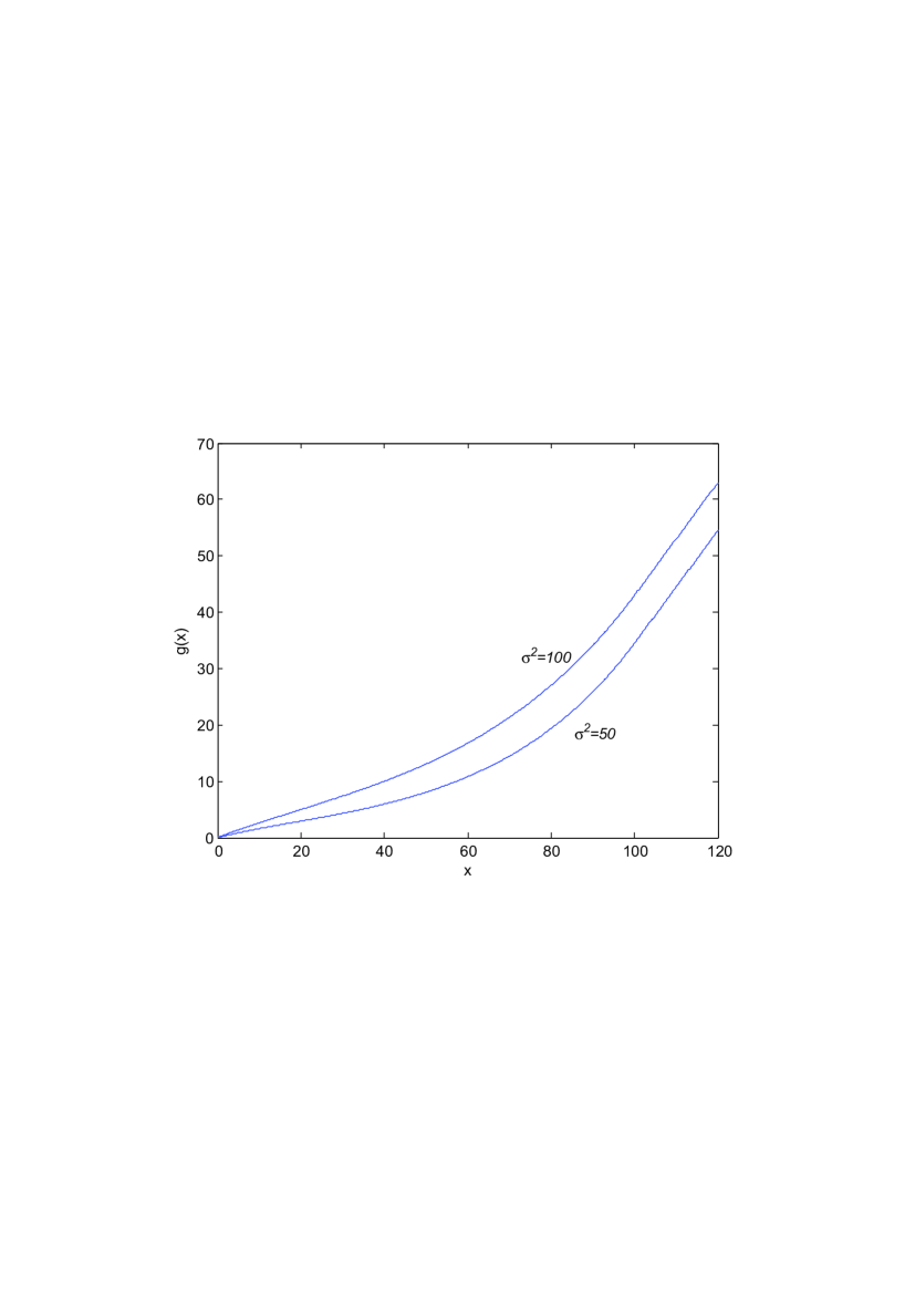
Figure 1. Value $g(x)$ as a function of $x$ in cases $\sigma^{2}=50$ and $\sigma^{2}=100$, respectively (parameters: $\mu=2$; $\lambda=6$; $c=0.05$; $b=100$)

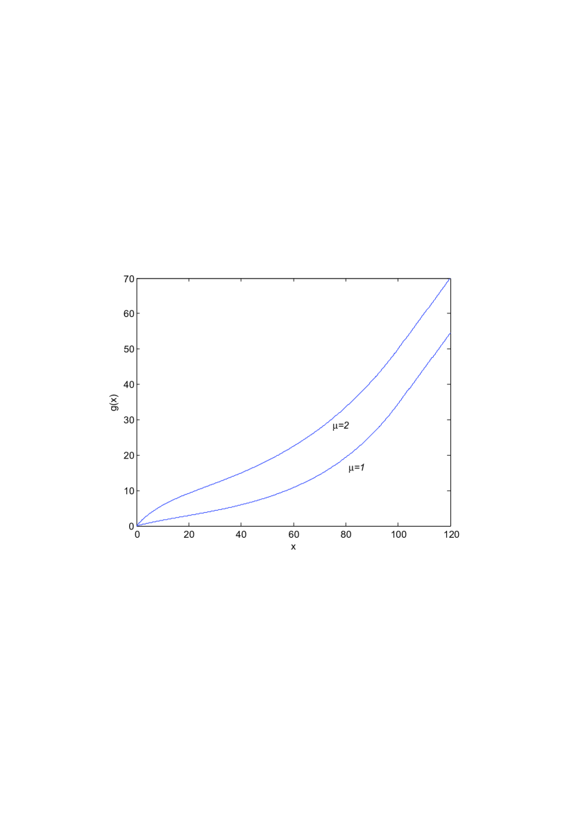
Figure 2. Value $g(x)$ as a function of $x$ in cases $\mu=1$ and $\mu=2$, respectively (parameters: $\sigma^{2}=50$; $\lambda=6$; $c=0.05$; $b=100$)

Example 5.2.

The graph 3 below shows that the probability of bankruptcy $\psi=1-\phi$ decreases with the initial capital $x$.

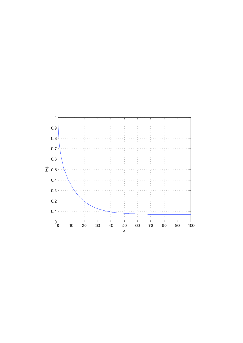
Figure 3. The probability of bankruptcy $\psi=1-\phi$ as a function of $x$ (parameters: $\sigma^{2}=50$; $\mu=2$; $\lambda=0.4$; $c=0.05$; $b=100$; $T=500$ )

Example 5.3.

The graph 4 below shows that the risk-based capital standard $x$ decreases with the preferred risk level $\varepsilon$. It states that the higher preferred risk level $\varepsilon$ needs a lower the initial risk-based capital.

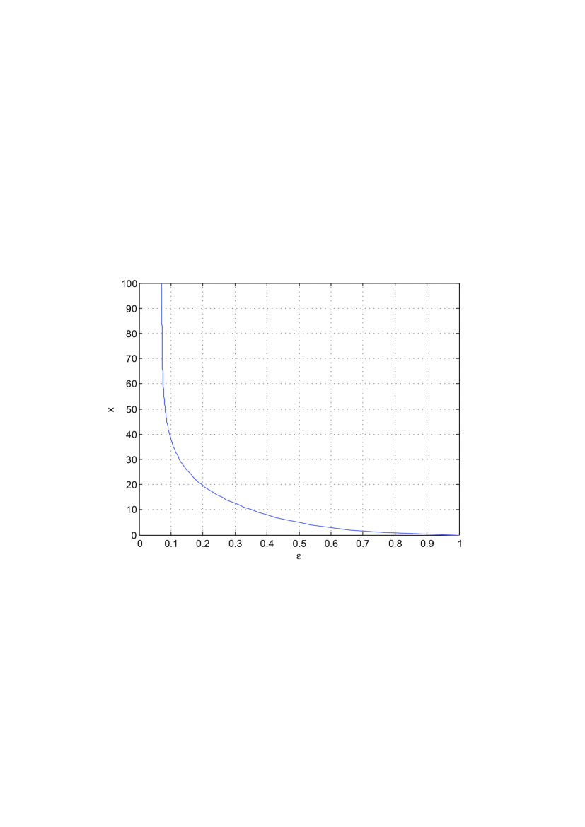
Figure 4. The risk-based capital standard $x$ as a function of $\varepsilon$(parameters: $\sigma^{2}=50$; $\mu=2$; $\lambda=0.4$; $c=0.05$; $b=100$; $T=500$)

Example 5.4.

The graphs 5 and 6 below show that the optimal dividend level $b(\varepsilon)$ is a decreasing function of the risk level $\varepsilon$. Inversely, the risk level $\varepsilon(b)$ is also a decreasing function of $b$.

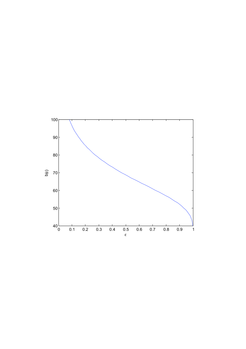
Figure 5. The optimal dividend level $b(\varepsilon)$ as a function of $\varepsilon$ (parameters: $\sigma^{2}=50$; $\mu=2$; $\lambda=0.4$; $c=0.05$; $b=100$; $T=500$ )

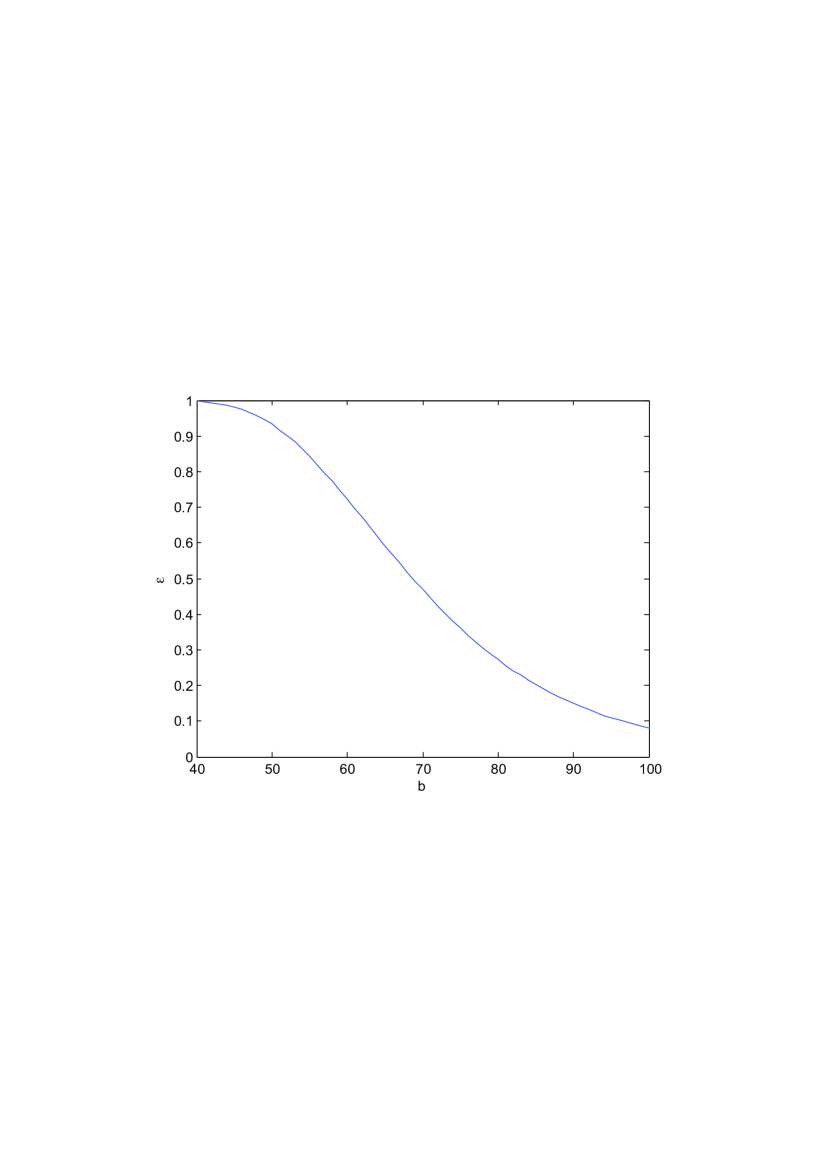
Figure 6. The risk level $\varepsilon(b)$ as a function of $b$ (parameters: $\sigma^{2}=50$; $\mu=2$; $\lambda=0.4$; $c=0.05$; $b=100$; $T=500$ )

6. Properties on the probability of bankruptcy

To give the proof of main result (Theorem 3.1) of this paper we list some lemmas on properties of the probability of bankruptcy in this section, and their detailed proofs will be given in section 8.

Lemma 6.1.

Assume that $\delta=\lambda-\mu>0$, $R^{\pi_{b}^{\ast},b}_{t}$ and $\tau_{b}^{\pi_{b}^{*}}$ are the same as in Lemma 4.2. Then the probability of bankruptcy $\mathbf{P}[\tau_{b}^{b}\leq T]$ is strictly decreasing on $[m,b_{K}]$,where $\tau_{b}^{b}:=\tau_{b}^{\pi_{b}^{*}}$ and $b_{K}:=\inf\{b:\mathbf{P}[\tau_{b}^{b}\leq T]=0\}$.

Proposition 6.1.

Assume that $\delta=\lambda-\mu>0$ and for any $b\geq b_{0}$ we define $R^{\pi_{b}^{\ast},y}_{t}$ by (4.5) with initial value $y$. Let $\phi^{b}(t,y)\in C^{1}(0,\infty)\cap C^{2}(0,b)$ and satisfy the following partial differential equation with boundary conditions,

$$\left\{\begin{array}[]{l l l}\phi_{t}^{b}(t,y)=\frac{1}{2}[A_{b}^{*}(y)]^{2}\sigma^{2}\phi_{yy}^{b}(t,y)+(\lambda A_{b}^{*}(y)-\delta)\phi_{y}^{b}(t,y),\\ \phi^{b}(0,y)=1,\ \mbox{for}\ \ 0<y\leq b,\\ \phi^{b}(t,0)=0,\phi_{y}^{b}(t,b)=0,\ \mbox{for}\ t>0.\end{array}\right.$$ (6.4)

Then $\phi^{b}(T,y)=1-\psi^{b}(T,y)$, i.e., $\phi^{b}(T,y)$ is probability that the company will survive on $[0,T]$, where $\psi^{b}(T,y)=\mathbf{P}\{\tau^{\pi_{b}^{\ast}}_{y}\leq T\}.$

Remark 6.1.

If we define $a(y):=\frac{1}{2}[A_{b}^{*}(y)]^{2}\sigma^{2}$, $\mu(y):=\lambda A_{b}^{*}(y)-\delta$, then the equation (6.4) becomes

$$\phi_{t}^{b}(t,y)=a(y)\phi_{yy}^{b}(t,y)+\mu(y)\phi_{y}^{b}(t,y).$$

By the properties of $A_{b}^{*}(y)$, we can easily show that $a(y)$ and $\mu(y)$ are continuous in $[0,b]$. So there exists a unique solution in $C^{1}(0,\infty)\cap C^{2}(0,b)$ for (6.4). Moreover, by Corollary A.1 in appendix, $a^{{}^{\prime}}(y)$, $\mu^{{}^{\prime}}(y)$ and $a^{{}^{\prime\prime}}(y)$ are bounded in $(0,m)$ and $(m,b)$.

The following, together with Proposition 6.1, states that the probability of bankruptcy $\psi^{b}(T,b):={\bf P}\big{\{}\tau_{b}^{\pi^{*}_{b}}<T\big{\}}$ is continuous with respect to $b(b\geq b_{0})$.

Lemma 6.2.

Assume that the same conditions as in Lemma 6.1. Let the function $\phi^{b}(t,x)$ solve the equation(6.4) and $u(b):=\phi^{b}(T,b)$. Then $u(b)$ is continuous with respect to $b(b\geq b_{0})$.

As a direct consequence of Theorem 4.2, Lemmas 6.1 and 6.2 we have the following.

Theorem 6.1.

For any fixed $\varepsilon>0$, there exists a unique $b^{*}$ satisfying ${\bf P}\big{\{}\tau_{b^{*}}^{\pi^{*}_{b^{*}}}<T\big{\}}=\varepsilon$.

7. Proof of Main Results

In this section we give the proof of the main results of this paper. we first need the following.

Theorem 7.1.

Let $V(x,b)$ and $V(x)$ be defined by (2) and (2.3), $f(x)$, $g(x)$ and $A^{*}_{b}(x)$ be the same as in Lemma A. 1 and Lemma A.2 in appendix, respectively. We have the following. (i) If $b\leq b_{0}$, then $V(x,b)=V(x,b_{0})=J(x,\pi_{b_{o}}^{\ast})=V(x,0)=f(x)$ and the optimal policy $\pi_{b_{o}}^{\ast}=\{A^{*}_{b_{0}}(R^{\pi_{b_{o}}^{\ast}}_{\cdot}),L^{\pi_{b_{o}}^{\ast}}_{\cdot}\}$ is uniquely determined by the following SDE:

$$\left\{\begin{array}[]{l l l}dR_{t}^{\pi_{b_{o}}^{\ast}}=(\mu-(1-A^{*}_{b_{0}}(R^{\pi_{b_{o}}^{\ast}}_{t}))\lambda)dt+\sigma A^{*}_{b_{0}}(R^{\pi_{b_{o}}^{\ast}}_{t})d{W}_{t}-dL_{t}^{\pi_{b_{o}}^{\ast}},\\ R_{0}^{\pi_{b_{o}}^{\ast}}=x,\\ 0\leq R^{\pi_{b_{o}}^{\ast}}_{t}\leq b_{0},\\ \int^{\infty}_{0}I_{\{t:R^{\pi_{b_{o}}^{\ast}}_{t}<b_{0}\}}(t)dL_{t}^{\pi_{b_{o}}^{\ast}}=0.\end{array}\right.$$ (7.5)

(ii) If $b\geq b_{0}$, then $V(x,b)=J(x,\pi^{*}_{b})=g(x)$ and the optimal policy $\pi_{b}^{\ast}=\{A^{*}_{b}(R^{\pi_{b}^{\ast}}_{\cdot}),L^{\pi_{b}^{\ast}}_{\cdot}\}$ is uniquely determined by the following SDE:

$$\left\{\begin{array}[]{l l l}dR_{t}^{\pi_{b}^{\ast}}=(\mu-(1-A^{*}_{b}(R^{\pi_{b}^{\ast}}_{t}))\lambda)dt+\sigma A^{*}_{b}(R^{\pi_{b}^{\ast}}_{t})d{W}_{t}-dL_{t}^{\pi_{b}^{\ast}},\\ R_{0}^{\pi_{b}^{\ast}}=x,\\ 0\leq R^{\pi_{b}^{\ast}}_{t}\leq b,\\ \int^{\infty}_{0}I_{\{t:R^{\pi_{b}^{\ast}}_{t}<b\}}(t)dL_{t}^{\pi_{b}^{\ast}}=0.\end{array}\right.$$ (7.10)

Proof.

(i) Assume that $b\leq b_{0}$. By using the fourth equality in (7.5), it follows that $\pi^{*}_{b_{0}}\in\Pi_{b_{0}}\subset\Pi_{b}$, so $V(x,b_{0})\leq V(x,b)\leq V(x,0)$. Therefore it suffices to prove that $V(x,0)\leq f(x)=V(x,b_{0})=J(x,\pi_{b_{o}}^{\ast})$. For any admissible policy $\pi=\{a_{\pi},L^{\pi}\}$, we assume that the process $(R^{\pi}_{t},L^{\pi}_{t})$ satisfies (2.1). Let $\Lambda=\{s:L_{s-}^{\pi}\neq L_{s}^{\pi}\}$ and $\hat{L}=\sum_{s\in\Lambda,s\leq t}(L_{s}^{\pi}-L_{s-}^{\pi})$ be the discontinuous part of $L_{s}^{\pi}$ and $\tilde{L}_{t}^{\pi}=L_{t}^{\pi}-\hat{L}_{t}^{\pi}$ be the continuous part of $L_{s}^{\pi}$, respectively. Define $\tau^{\varepsilon}=\inf\{t\geq 0:R^{\pi}_{t}\leq\varepsilon\}$. By applying generalized Itô formula to stochastic process $R^{\pi}_{t}$ and the function $f(x)$, we get

$$e^{-c(t\wedge\tau^{\varepsilon})}f(R_{t\wedge\tau^{\varepsilon}}^{\pi}) = f(x)+\int_{0}^{t\wedge\tau^{\varepsilon}}e^{-cs}\mathcal{L}f(R_{s}^{\pi})ds$$ (7.11)

$$+ \int_{0}^{t\wedge\tau^{\varepsilon}}a_{\pi}\sigma e^{-cs}f^{{}^{\prime}}(R_{s}^{\pi})d{W}_{s}\mathcal{-}\int_{0}^{t\wedge\tau^{\varepsilon}}e^{-cs}f^{{}^{\prime}}(R_{s}^{\pi})dL_{s}^{\pi}$$

$$+ \sum\limits_{s\in\Lambda,s\leq t\wedge\tau^{\varepsilon}}e^{-cs}[f(R_{s}^{\pi})-f(R_{s-}^{\pi})$$

$$- f^{{}^{\prime}}(R_{s-}^{\pi})(R_{s}^{\pi}-R_{s-}^{\pi})]$$

$$= f(x)+\int_{0}^{t\wedge\tau^{\varepsilon}}e^{-cs}\mathcal{L}f(R_{s}^{\pi})ds$$

$$+ \int_{0}^{t\wedge\tau^{\varepsilon}}a_{\pi}\sigma e^{-cs}f^{{}^{\prime}}(R_{s}^{\pi})d{W}_{s}\mathcal{-}\int_{0}^{t\wedge\tau^{\varepsilon}}e^{-cs}f^{{}^{\prime}}(R_{s}^{\pi})d\tilde{L}_{s}^{\pi}$$

$$+ \sum\limits_{s\in\Lambda,s\leq t\wedge\tau^{\varepsilon}}e^{-cs}[f(R_{s}^{\pi})-f(R_{s-}^{\pi}))],$$

where

$$\mathcal{L}=\frac{1}{2}a^{2}\sigma^{2}\frac{d^{2}}{dx^{2}}+(\mu-(1-a)\lambda)\frac{d}{dx}-c.$$

By the (9.17) and $f^{{}^{\prime}}(R_{s\wedge\tau^{\varepsilon}}^{\pi})\leq f^{{}^{\prime}}(\varepsilon)$, the second term and third term on the right hand side of (7.11) is non-positive and a square integrable martingale, respectively, therefore, by taking mathematical expectations at both sides of (7.11) and letting $\varepsilon\rightarrow 0$, we have

$${\bf E}\big{\{}e^{-c(t\wedge\tau^{\pi}_{x})}f(R_{t\wedge\tau^{\pi}_{x}}^{\pi})\big{\}} \leq f(x)-{\bf E}\big{\{}\int_{0}^{t\wedge\tau^{\pi}_{x}}e^{-cs}f^{{}^{\prime}}(R_{s}^{\pi})d\tilde{L}_{s}^{\pi}\big{\}}$$

$$+ {\bf E}\big{\{}\sum\limits_{s\in\Lambda,s\leq t\wedge\tau^{\pi}_{x}}e^{-cs}[f(R_{s}^{\pi})-f(R_{s-}^{\pi})]\big{\}}.$$

Since $f^{{}^{\prime}}(R_{s}^{\pi})\geq 1$ for $x\geq 0$,

$$f(R_{s}^{\pi})-f(R_{s-}^{\pi})\leq-(L_{s}^{\pi}-L_{s-}^{\pi}),$$ (7.13)

which, together with (7), implies that

$${\bf E}\big{\{}e^{-c(t\wedge\tau^{\pi}_{x})}f(R_{t\wedge\tau^{\pi}_{x}}^{\pi})\big{\}} + {\bf E}\big{\{}\int_{0}^{t\wedge\tau^{\pi}_{x}}e^{-cs}dL_{s}^{\pi}\big{\}}\leq f(x).$$ (7.14)

By definition of $\tau^{\pi}_{x}$ and $f(0)=0$, it is easy to prove that

$$\liminf\limits_{t\rightarrow\infty}e^{-c(t\wedge\tau^{\pi}_{x})}f(R_{t\wedge\tau^{\pi}_{x}}^{\pi}) = e^{-c\tau}f(0)I_{\{\tau^{\pi}_{x}<\infty\}}$$ (7.15)

$$+ \liminf\limits_{t\rightarrow\infty}e^{-ct}f(R_{t})I_{\{\tau^{\pi}_{x}=\infty\}}\geq 0.$$

So we see from (7.15) and (7.14) that

$$J(x,\pi)={\bf E}[\big{\{}\int_{0}^{\tau^{\pi}_{x}}e^{-cs}dL_{s}^{\pi}\}]\leq f(x).$$

Thus

$$V(x,0)\leq f(x).$$ (7.16)

If we let policy $\pi_{b_{o}}^{\ast}=\{A^{*}_{b_{0}}(R^{\pi_{b_{o}}^{\ast}}_{\cdot}),L^{\pi_{b_{o}}^{\ast}}_{\cdot}\}$ , which is uniquely determined by SDE(7.5), see Lions and Sznitman[20], then $R^{\pi_{b_{o}}^{\ast}}_{t}$ and $L^{\pi_{b_{o}}^{\ast}}_{t}$ are continuous stochastic processes. So all the inequalities above become equalities and

$$V(x,0)\leq f(x)=V(x,b_{0})=J(x,\pi_{b_{o}}^{\ast}).$$

The proof of the part (i) follows.

(b) We assume that $b\geq b_{0}$. For any $\pi\in\Pi_{b}$, let $(R^{\pi}_{t},L^{\pi}_{t})$ satisfies (2.1). It is easy to see from the definition of $\Pi_{b}$ that

$$\left\{\begin{array}[]{l l l}\mathbf{P}\{R_{s-}^{\pi}\geq R_{s}^{\pi}\geq b\}+\mathbf{P}\{b\geq R_{s-}^{\pi}\geq R_{s}^{\pi}\}=1,\ \forall s\geq 0,\\ \mathcal{L}g(R_{s}^{\pi})\leq 0\ \mbox{for $s\leq\tau^{\pi}_{x}=\inf\{t\geq 0:R^{\pi}_{s}\leq 0\}$},\\ g^{\prime}(x)=1\ \mbox{for $x\geq b$}.\end{array}\right.$$ (7.20)

By using (7.20), we have (7.13) with replacing $f$ by $g$. Then by the same way as in (i),

$$V(x,b)\leq g(x).$$

Choosing the policy $\pi_{b}^{\ast}=\{A^{*}_{b}(R^{\pi_{b}^{\ast}}_{\cdot}),L^{\pi_{b}^{\ast}}_{\cdot}\}$, which is uniquely determined by SDE(7.10), yields that the last inequality becomes equality. Thus the proof is complete. ∎

Now we give the proof of main result (Theorem 3.1) of this paper.

Proof.

If $\mathbf{P}[\tau_{b_{0}}^{\pi^{*}_{b_{0}}}\leq T]\leq\varepsilon$, then the conclusion follows from the part (i) of Theorem 7.1. If $\mathbf{P}[\tau_{b_{0}}^{\pi^{*}_{b_{0}}}\leq T]>\varepsilon$, then, by Theorem 4.2, Lemmas 6.1 and 6.2, the equation $\mathbf{P}\{\tau_{b}^{\pi^{*}_{b}}\leq T\}=\varepsilon$ has a unique solution $b^{\ast}$ and $b^{\ast}=\inf\{b:b\in\mathfrak{B}\}>b_{0}$. By Theorem 7.1 and Corollary A.2 in appendix, $g(x,b)=V(x,b)$ is decreasing w.r.t.$b(\geq b_{0})$, so (3.6) follows from the part (ii) of Theorem 7.1. Moreover, $g(x,b^{*})(=V(x,b^{*}))$ is the value function of the company, the optimal policy associated with $g(x)=g(x,b^{*})$ is $\pi_{b^{*}}^{\ast}=\{A^{*}_{b^{*}}(R^{\pi_{b^{*}}^{\ast}}_{\cdot}),L^{\pi_{b^{*}}^{\ast}}_{\cdot}\}$ which is uniquely determined by SDE(7.10). The inequality (3.13) is a direct consequence of Corollary A.2 in appendix. Thus we complete the proof. ∎

8. Proof of Lemmas and Proposition

${\sl ProofofLemma\ \ref{lemma52}}$. We only prove Lemma 6.1 in case of $\mu<\lambda<2\mu$ because other case can be treated similarly. We prove that the probability of bankruptcy is strictly decreasing on $[m,b_{K}]$, that is,

$$\mathbf{P}[\tau_{b_{1}}^{b_{1}}\leq T]-\mathbf{P}[\tau_{b_{2}}^{b_{2}}\leq T]>0$$

for any $b_{2}>b_{1}\geq m$. By comparison theorem,

$$\mathbf{P}[\tau_{b_{1}}^{b_{1}}\leq T]-\mathbf{P}[\tau_{b_{2}}^{b_{2}}\leq T]\geq\mathbf{P}[\tau_{b_{1}}^{b_{2}}\leq T]-\mathbf{P}[\tau_{b_{2}}^{b_{2}}\leq T].$$

The proof can be reduced to proving that

$$\mathbf{P}[\tau_{b_{1}}^{b_{2}}\leq T]-\mathbf{P}[\tau_{b_{2}}^{b_{2}}\leq T]>0.$$ (8.1)

To prove the inequality (8.1) we define stochastic processes $R_{t}^{[1]}$ and $R_{t}^{[2]}$ by the following SDEs:

$$dR_{t}^{[1]}=[A_{b_{2}}^{*}(R_{t}^{[1]})\lambda-\delta]dt+A_{b_{2}}^{*}(R_{t}^{[1]})\sigma d\mathcal{W}_{t}-dL_{t}^{b_{2}},R_{0}^{[1]}=b_{1},$$

$$dR_{t}^{[2]}=[A_{b_{2}}^{*}(R_{t}^{[2]})\lambda-\delta]dt+A_{b_{2}}^{*}(R_{t}^{[2]})\sigma d\mathcal{W}_{t}-dL_{t}^{b_{2}},R_{0}^{[2]}=b_{2},$$

respectively.Let $\tau^{b_{1}}=\inf\limits_{t\geq 0}\{t:R_{t}^{[2]}=b_{1}\}$, $A=\{\tau^{b_{1}}\leq T\}$ and $B=\big{\{}\sl R_{t}^{[2]}$ will go to bankruptcy in a time interval $[\tau^{b_{1}},\tau^{b_{1}}+T]$ and $\tau^{b_{1}}\leq T\big{\}}$. Then $\{\tau_{b_{2}}^{b_{2}}\leq T\}\subset B$. Moreover, by using strong Markov property of $R_{t}^{[2]}$, we have

$$\mathbf{P}[\tau_{b_{1}}^{b_{2}}\leq T]=\mathbf{P}[B|A].$$

So

$$\mathbf{P}[\tau_{b_{1}}^{b_{2}}\leq T]-\mathbf{P}[\tau_{b_{2}}^{b_{2}}\leq T] \geq \mathbf{P}[\tau_{b_{1}}^{b_{2}}\leq T]-\mathbf{P}(B)$$

$$= \mathbf{P}[\tau_{b_{1}}^{b_{2}}\leq T]-\mathbf{P}(A)\mathbf{P}(B|A)$$

$$= \mathbf{P}[\tau_{b_{1}}^{b_{2}}\leq T](1-\mathbf{P}(A))$$

$$= \mathbf{P}[\tau_{b_{1}}^{b_{2}}\leq T]\mathbf{P}(A^{c}).$$

By Theorem 4.1, $\mathbf{P}[\tau_{b_{1}}^{b_{2}}\leq T]>0$. Hence we only need to prove $\mathbf{P}(A^{c})>0$. For doing this we define stochastic processes $R_{t}^{[3]}$ and $R_{t}^{[4]}$ by the following SDEs:

$$\left\{\begin{array}[]{l l l}dR_{t}^{[3]}=[A_{b_{2}}^{*}(R_{t}^{[3]})\lambda-\delta]dt+A_{b_{2}}^{*}(R_{t}^{[3]})\sigma d\mathcal{W}_{t}-dL_{t}^{b_{2}},\\ R_{0}^{[3]}=\frac{b_{1}+b_{2}}{2},\end{array}\right.$$

$$\left\{\begin{array}[]{l l l}dR_{t}^{[4]}=[A_{b_{2}}^{*}(R_{t}^{[4]})\lambda-\delta]dt+A_{b_{2}}^{*}(R_{t}^{[4]})\sigma d{W}_{t},\\ R_{0}^{[4]}=\frac{b_{1}+b_{2}}{2}.\end{array}\right.$$

Setting $D=\{\inf\limits_{0\leq t\leq T}R_{t}^{[3]}>b_{1}\}$ and $E=\{\inf\limits_{0\leq t\leq T}R_{t}^{[4]}>b_{1},\sup\limits_{0\leq t\leq T}R_{t}^{[4]}<b_{2}\}$, by comparison theorem on SDE, we have $\mathbf{P}(A^{c})\geq\mathbf{P}(D)\geq\mathbf{P}(E)$. Since $A_{b_{2}}^{*}(x)=1$ for any $x>m$,

$$R_{t}^{[4]}=\frac{b_{1}+b_{2}}{2}+[\lambda-\delta]t+\sigma{W}_{t}\ \mbox{ on $E$}.$$ (8.4)

We deduce from (8.4) and properties of Brownian motion with drift (cf. Borodin and Salminen [1] (2002)) that

$$\mathbf{P}(E)=\frac{e^{-\mu^{\prime 2}T/2}}{\sqrt{2\pi T}}\sum_{k=-\infty}^{\infty}\int_{b_{1}/\sigma}^{b_{2}/\sigma}e^{\mu^{\prime}(z-x)}[(e^{-(z-x+\frac{2k(b_{2}-b_{1})}{\sigma})^{2}/2T})$$

$$-(e^{-(z+x-\frac{2b_{1}-2k(b_{2}-b_{1})}{\sigma})^{2}/2T})]dz>0,$$

where $\mu^{\prime}=(\lambda-\delta)/\sigma$ and $x=\frac{b_{1}+b_{2}}{2\sigma}$. Thus the proof follows.   $\Box$

${\sl ProofofProposition\ \ref{proposition51}}$.  Let $\phi(t,y)\equiv\phi^{b}(t,y)$. Since the stochastic process $(R^{\pi_{b}^{\ast},y}_{t},L_{t}^{\pi_{b}^{\ast}})$ is continuous, by applying the generalized Itô formula to $(R^{\pi_{b}^{\ast},y}_{t},L_{t}^{\pi_{b}^{\ast}})$ and $\phi(t,y)$, we have for $0<y\leq b$

$$\phi(T-(t\wedge\tau_{y}^{b}),R^{\pi_{b}^{\ast},y}_{t\wedge\tau_{y}^{b}}) = \phi(T,y)$$ (8.5)

$$+ \int_{0}^{t\wedge\tau_{y}^{b}}(\frac{1}{2}A_{b}^{*2}(R^{\pi_{b}^{\ast},y}_{s})\sigma^{2}\phi_{yy}(T-s,R^{\pi_{b}^{\ast},y}_{s})$$

$$+ (\lambda A^{*}_{b}(R^{\pi_{b}^{\ast},y}_{s})-\delta)\phi_{y}(T-s,R^{\pi_{b}^{\ast},y}_{s})$$

$$- \phi_{t}(T-s,R^{\pi_{b}^{\ast},y}_{s}))ds-\int_{0}^{t\wedge\tau_{y}^{b}}\phi_{y}(T-s,R^{\pi_{b}^{\ast},y}_{s})dL_{s}^{b}$$

$$+ \int_{0}^{t\wedge\tau_{y}^{b}}A_{b}^{*}(R^{\pi_{b}^{\ast},y}_{s})\sigma\phi_{y}(T-s,R^{\pi_{b}^{\ast},y}_{s})dW_{s},$$

where $\tau_{y}^{b}\equiv\tau^{\pi_{b}^{\ast}}_{y}=\inf\{t:R^{\pi_{b}^{\ast},y}_{t}=0\}$.
Letting $t=T$ and taking mathematical expectation at both sides of (8.5) yield that

$$\phi(T,y) = \mathbf{E}[\phi(T-(T\wedge\tau_{y}^{b}),R^{\pi_{b}^{\ast},y}_{T\wedge\tau_{y}^{b}})]$$

$$= \mathbf{E}[\phi(0,R^{\pi_{b}^{\ast},y}_{T})1_{T<\tau_{y}^{b}}]+\mathbf{E}[\phi(T-\tau_{y}^{b},0)1_{T\geq\tau_{y}^{b}})]$$

$$= \mathbf{E}[1_{T<\tau_{y}^{b}}]=1-\psi(T,y).$$

$\Box$

Finally, we will use PDE method to prove that the probability of bankruptcy $\psi^{b}(T,b)\>={\bf P}\big{\{}\tau_{b}^{\pi^{*}_{b}}<T\big{\}}$ is continuous w.r.t. $b$.

${\sl ProofofLemma\ \ref{lemma53}}$. It suffices to prove that $\phi^{b}(t,x)$ is continuous in $b$. Let $y=bz$ and $\theta^{b}(t,z)=\phi^{b}(t,by)$, the equation (6.4) becomes

$$\left\{\begin{array}[]{l l l}\theta_{t}^{b}(t,z)=[a(bz)/b^{2}]\theta_{zz}^{b}(t,z)+[\mu(bz)/b]\theta_{z}^{b}(t,z),\\ \theta^{b}(0,z)=1,\ \mbox{for}\ 0<z\leq 1,\\ \theta^{b}(t,0)=0,\theta_{z}^{b}(t,1)=0,\ \mbox{for}\ t>0.\end{array}\right.$$

So the proof of Lemma 6.2 reduces to proving $\lim\limits_{b_{2}\rightarrow b_{1}}\theta^{b_{2}}(t,z)=\theta^{b_{1}}(t,z)$ for fixed $b_{1}>b_{0}$. Setting $w(t,z)=\theta^{b_{2}}(t,z)-\theta^{b_{1}}(t,z)$, we have

$$\left\{\begin{array}[]{l l l}w_{t}(t,z)&=&[a(b_{2}z)/b_{2}^{2}]w_{zz}(t,z)+[\mu(b_{2}z)/b_{2}]w_{z}(t,z)\\ &+&\{a(b_{2}z)/b_{2}^{2}-a(b_{1}z)/b_{1}^{2}\}\theta_{zz}^{b_{1}}(t,z)\\ &+&\{a(b_{2}z)/b_{2}^{2}-a(b_{1}z)/b_{1}^{2}\}\theta_{z}^{b_{1}}(t,z),\\ w(0,z)&=&0,\ \mbox{for}\ 0<z\leq 1,\\ w(t,0)&=&0,\ w_{x}(t,1)=0,\ \mbox{for}\ t>0.\end{array}\right.$$ (8.12)

By multiplying the first equation in (8.12) by $w(t,z)$ and then integrating on $[0,t]\times[0,1]$,

$$\int_{0}^{t}\int_{0}^{1}w(s,x)w_{t}(s,x)dxds$$ (8.13)

$$= \int_{0}^{t}\int_{0}^{1}\big{\{}[a(b_{2}x)/b_{2}^{2}]w(s,x)w_{xx}(s,x)$$

$$+ [\mu(b_{2}x)/b_{2}]w(s,x)w_{x}(s,x)$$

$$+ [a(b_{2}x)/b_{2}^{2}-a(b_{1}x)/b_{1}^{2}]w(s,x)\theta_{xx}^{b_{1}}(t,x)$$

$$+ w(s,x)[\mu(b_{2}x)/b_{2}-\mu(b_{1}x)/b_{1}]w(s,x)\theta_{x}^{b_{1}}(t,x)\big{\}}dxds$$

$$\equiv E_{1}+E_{2}+E_{3}+E_{4}.$$

We now estimate terms $E_{i}$, $i=1,\cdots,4$, at both sides of (8.13) as follows. Firstly,

$$\int_{0}^{t}\int_{0}^{1}w(s,x)w_{t}(s,x)dxds = \int_{0}^{1}\frac{1}{2}w^{2}(t,x)dx.$$ (8.14)

Secondly, by Corollary A.1 in appendix and definitions of $a(x)$ and $\mu(x)$, there exit positive constants $D_{1}$, $D_{2}$ and $D_{3}$ such that $[\mu(b_{2}z)/b_{2}]^{2}\leq D_{1}$, $[a(bx)/b^{2}]^{\prime}\geq 0$, $[a(b_{2}x)/b_{2}^{2}]\geq D_{2}$ and $[a(b_{2}x)/b_{2}^{2}]^{\prime}\leq D_{3}$, so by Young’s inequality, we have for any $\lambda_{1}>0$ and $\lambda_{2}>0$

$$E_{1} = \int_{0}^{t}\int_{0}^{1}[a(b_{2}x)/b_{2}^{2}]w(s,x)w_{xx}(s,x)dxds$$ (8.15)

$$= -\int_{0}^{t}\int_{0}^{1}[a(b_{2}x)/b_{2}^{2}]w_{x}^{2}(s,x)dxds$$

$$-\int_{0}^{t}\int_{0}^{m/b_{2}}[a(b_{2}x)/b_{2}^{2}]^{{}^{\prime}}w_{x}(s,x)w(s,x)dxds$$

$$\leq -D_{2}\int_{0}^{t}\int_{0}^{1}w_{x}^{2}(s,x)dxds$$

$$+D_{3}\int_{0}^{t}\int_{0}^{1}[\lambda_{1}w_{x}^{2}(s,x)+\frac{1}{4\lambda_{1}}w^{2}(s,x)]dxds$$

and

$$E_{2} = \int_{0}^{t}\int_{0}^{1}[\mu(b_{2}x)/b_{2}]w(s,x)w_{x}(s,x)dxds$$ (8.16)

$$\leq \lambda_{2}\int_{0}^{t}\int_{0}^{1}w_{x}^{2}(s,x)dxds$$

$$+\frac{D_{1}}{4\lambda_{2}}\int_{0}^{t}\int_{0}^{1}w^{2}(s,x)dxds.$$

Thirdly, it is easy to see from Corollary A.1 in appendix that $[a(bx)/b^{2}]$, $[a(bx)/b^{2}]^{\prime}$and $[\mu(bx)/b]$ are Lipschitz continuous for all $x\in(x_{1}/b_{2},x_{2}/b_{1})$, that is, there exists an $L>0$ such that

$$\left\{\begin{array}[]{l l l}|[a(b_{2}x)/b_{2}^{2}]-[a(b_{1}x)/b_{1}^{2}]|\leq L|b_{2}-b_{1}|,\\ |[a(b_{2}x)/b_{2}^{2}]^{\prime}-[a(b_{1}x)/b_{1}^{2}]^{\prime}|\leq L|b_{2}-b_{1}|,\\ |[\mu(b_{2}x)/b_{2}]-[\mu(b_{1}x)/b_{1}]|\leq L|b_{2}-b_{1}|.\end{array}\right.$$ (8.20)

Noting that $E_{3}$ has the following expressions:

$$E_{3} = \int_{0}^{t}\int_{0}^{1}\{a(b_{2}x)/b_{2}^{2}-a(b_{1}x)/b_{1}^{2}\}w(s,x)\theta_{xx}^{b_{1}}(s,x)dxds$$ (8.21)

$$= -\int_{0}^{t}\int_{0}^{1}\{a(b_{2}x)/b_{2}^{2}-a(b_{1}x)/b_{1}^{2}\}w_{x}(s,x)\theta_{x}^{b_{1}}(s,x)dxds$$

$$-\int_{0}^{t}\{\int_{0}^{m/b_{2}}\{a(b_{2}x)/b_{2}^{2}-a(b_{1}x)/b_{1}^{2}\}^{\prime}w(s,x)\theta_{x}^{b_{1}}(s,x)dx$$

$$-\int_{m/b_{2}}^{m/b_{1}}\{a(b_{2}x)/b_{2}^{2}-a(b_{1}x)/b_{1}^{2}\}^{\prime}w(s,x)\theta_{x}^{b_{1}}(s,x)dx$$

$$-\int_{m/b_{1}}^{1}\{a(b_{2}x)/b_{2}^{2}-a(b_{1}x)/b_{1}^{2}\}w(s,x)^{\prime}\theta_{x}^{b_{1}}(s,x)dx\}ds$$

$$= -\int_{0}^{t}\int_{0}^{1}\{a(b_{2}x)/b_{2}^{2}-a(b_{1}x)/b_{1}^{2}\}w_{x}(s,x)\theta_{x}^{b_{1}}(s,x)dxds$$

$$-\int_{0}^{t}\{\int_{0}^{m/b_{2}}\{a(b_{2}x)/b_{2}^{2}-a(b_{1}x)/b_{1}^{2}\}^{\prime}w(s,x)\theta_{x}^{b_{1}}(s,x)dx$$

$$-\int_{m/b_{2}}^{m/b_{1}}\{a(b_{2}x)/b_{2}^{2}-a(b_{1}x)/b_{1}^{2}\}^{\prime}w(s,x)\theta_{x}^{b_{1}}(s,x)\}dsdx$$

$$= E_{31}+E_{32}+E_{33},$$

$$\lim_{b_{2}\rightarrow b_{1}}\{|E_{33}|\}=0,$$

and using (8.20), by the same way as in (8.15) and (8.16), we have for any $\lambda_{3}>0$ and $\lambda_{4}>0$

$$E_{31} = -\int_{0}^{t}\int_{0}^{1}\{a(b_{2}x)/b_{2}^{2}-a(b_{1}x)/b_{1}^{2}\}w(s,x)\theta_{x}^{b_{1}}(s,x)dxds$$

$$\leq \frac{L^{2}(b_{2}-b_{1})^{2}}{4\lambda_{3}}\int_{0}^{t}\int_{0}^{1}[\theta_{x}^{b_{1}}(s,x)]^{2}dxds$$

$$+\lambda_{3}\int_{0}^{t}\int_{0}^{1}[w_{x}^{2}(s,x)+w^{2}(s,x)]dxds$$

and

$$E_{32} = -\int_{0}^{t}\int_{0}^{m/b_{2}}\{a(b_{2}x)/b_{2}^{2}-a(b_{1}x)/b_{1}^{2}\}^{\prime}w(s,x)\theta_{x}^{b_{1}}(s,x)dxds$$

$$\leq \frac{L^{2}(b_{2}-b_{1})^{2}}{4\lambda_{4}}\int_{0}^{t}\int_{0}^{1}[\theta_{x}^{b_{1}}(s,x)]^{2}dxds$$

$$+\lambda_{4}\int_{0}^{t}\int_{0}^{1}[w_{x}^{2}(s,x)+w^{2}(s,x)]dxds.$$

By Corollary A.1 in appendix, there exists a constant $D_{4}>0$ such that $|[a(bz)/b^{2}]^{\prime}-[\mu(bx)/b]|\leq D_{4}$ and $\lambda_{5}=\inf\limits_{b_{1}\leq b\leq b_{2}}\{a(bx)/b^{2}\}>0$. Then, by the boundary conditions, we estimate $\int_{0}^{t}\int_{0}^{1}[\theta_{x}^{b}(s,x)]^{2}dxds$ for $b\in[b_{1},b_{2}]$ as follows:

$$0 = \int_{0}^{t}\int_{0}^{1}\theta_{t}^{b}(s,x)\theta^{b}(s,x)$$

$$-[a(bx)/b^{2}]\theta_{xx}^{b}(s,x)\theta^{b}(s,x)-[\mu(bx)/b]\theta_{x}^{b}(s,x)\theta^{b}(s,x)dxds$$

$$= \frac{1}{2}\int_{0}^{1}[\theta^{b}(s,x)]^{2}dx+\int_{0}^{t}\int_{0}^{1}[a(bx)/b^{2}][\theta_{x}^{b}(s,x)]^{2}dxds$$

$$+\int_{0}^{t}\int_{0}^{1}[a(bx)/b^{2}]^{\prime}[\theta_{x}^{b}(s,x)][\theta^{b}(s,x)]dxds$$

$$-\int_{0}^{t}\int_{0}^{1}[\mu(bx)/b][\theta_{x}^{b}(s,x)][\theta^{b}(s,x)]dxds$$

$$\geq \lambda_{5}\int_{0}^{t}\int_{0}^{1}[\theta_{x}^{b}(s,x)]^{2}dxds-\frac{\lambda_{5}}{2}\int_{0}^{t}\int_{0}^{1}[\theta_{x}^{b}(s,x)]^{2}dxds$$

$$-\frac{1}{2\lambda_{5}}\int_{0}^{t}\int_{0}^{1}[\theta^{b}(s,x)]^{2}dxds$$

$$\geq \frac{\lambda_{5}}{2}\int_{0}^{t}\int_{0}^{1}[\theta_{x}^{b}(s,x)]^{2}dxds-\frac{D_{4}}{2\lambda_{5}}$$

from which we see that

$$\int_{0}^{t}\int_{0}^{1}[\theta_{x}^{b}(s,x)]^{2}dxds\leq\frac{\lambda_{5}^{2}}{D_{4}}.$$

Therefore we conclude that there exists a positive function $B^{b_{1}}(b_{2})$ such that

$$\lim\limits_{b_{2}\rightarrow b_{1}}B^{b_{1}}(b_{2})=0$$

and for $0\leq t\leq T$

$$E_{3} = \int_{0}^{t}\int_{0}^{1}\{a(b_{2}x)/b_{2}^{2}-a(b_{1}x)/b_{1}^{2}\}w(s,x)\theta_{xx}^{b_{1}}(t,x)dxds$$ (8.22)

$$\leq B^{b_{1}}(b_{2})+(\lambda_{3}+\lambda_{4})\int_{0}^{t}\int_{0}^{1}[w_{x}^{2}(s,x)+w^{2}(s,x)]dxds.$$

Finally, by using the same way as in estimating $E_{3}$, we can find a positive function $B_{1}^{b_{1}}(b_{2})$ such that

$$\lim\limits_{b_{2}\rightarrow b_{1}}B_{1}^{b_{1}}(b_{2})=0$$

and for any $\lambda_{6}>0$

$$E_{4} = \int_{0}^{t}\int_{0}^{1}\{\mu(b_{2}x)/b_{2}-\mu(b_{1}x)/b_{1}\}w(s,x)\theta_{x}^{b_{1}}(t,x)dxds$$ (8.23)

$$\leq B_{1}^{b_{1}}(b_{2})+\lambda_{6}\int_{0}^{t}\int_{0}^{1}w^{2}(s,x)dxds.$$

By choosing $\lambda_{1}$, $\lambda_{2}$, $\lambda_{3}$ and $\lambda_{4}$ such that $\lambda_{2}+\lambda_{1}D_{3}+\lambda_{3}+\lambda_{4}\leq D_{2}$ , it see from (8.13), (8.15)-(8.23) that there exist positive constants $C_{1}$ and $C_{2}$ such that

$$\int_{0}^{1}w^{2}(t,x)dx\leq C_{1}\int_{0}^{t}\int_{0}^{1}w^{2}(s,x)dxds+C_{2}[B_{1}^{b_{1}}(b_{2})+B^{b_{1}}(b_{2})].$$

By setting $F(t)=\int_{0}^{t}\int_{0}^{1}w^{2}(s,x)dxds$ and using the Gronwall inequality, we get

$$F(t)\leq C_{2}[B_{1}^{b_{1}}(b_{2})+B^{b_{1}}(b_{2})]\exp\{C_{1}t\}.$$

So

$$\lim\limits_{b_{2}\rightarrow b_{1}}\int_{0}^{t}\int_{0}^{1}[\theta^{b_{2}}(s,x)-\theta^{b_{1}}(s,x)]^{2}dxds=0.$$

Thus the proof has been done.   $\Box$

9. Appendix

The appendix lists the solutions of the two HJB equations and properties of them. Since the procedure of solving the two equations is completely similar to that of Taksar and Zhou[24](1998), we omit it.

Lemma A 1.

Assume that $f(x)\in C^{2}$ satisfies the following HJB equation and boundary conditions:

$$\left\{\begin{array}[]{l l l}\max\limits_{a\in[0,1]}[\frac{1}{2}\sigma^{2}a^{2}f^{{}^{\prime\prime}}(x)+(\mu-(1-a)\lambda)f^{{}^{\prime}}(x)-cf(x)]=0,\ 0\leq x\leq b_{0},\\ f^{{}^{\prime}}(x)=1,\ \mbox{ for}\ x\geq b_{0},\\ f^{{}^{\prime\prime}}(x)=0,\ \mbox{ for}\ x\geq b_{0},\\ f(0)=0.\end{array}\right.$$ (9.5)

(i) If $\lambda\geq 2\mu$, then

$$f(x)=\left\{\begin{array}[]{l l l}f_{1}(x,b_{0})=C_{0}(b_{0})(e^{\zeta_{1}x}-e^{\zeta_{2}x}),&x\leq b_{0},\\ f_{2}(x,b_{0})=C_{0}(b_{0})(e^{\zeta_{1}b_{0}}-e^{\zeta_{2}b_{0}})+x-b_{0},&x\geq b_{0}.\end{array}\right.$$ (9.8)

If $\mu<\lambda<2\mu$, then

$$f(x)=\left\{\begin{array}[]{l l l}f_{3}(x,b_{0})=\int_{0}^{x}X^{-1}(y)dy,\ x\leq m,\\ f_{4}(x,b_{0})=\frac{C_{1}(b_{0})}{\zeta_{1}}\exp{(\zeta_{1}(x-m))}+\frac{C_{2}(b_{0})}{\zeta_{2}}\exp{(\zeta_{2}(x-m))},\\ \ m<x<b_{0},\\ f_{5}(x,b_{0})=\frac{C_{1}(b_{0})}{\zeta_{1}}\exp{(\zeta_{1}(b_{0}-m))}+\frac{C_{2}(b_{0})}{\zeta_{2}}\exp\{\zeta_{2}(b_{0}-m)\}\\ \qquad\qquad\quad+x-b_{0},\ x\geq b_{0}.\end{array}\right.$$ (9.14)

(ii)

$$\left\{\begin{array}[]{l l l}\max\mathcal{L}f(x)\leq 0\ \mbox{and }\ f^{{}^{\prime}}(x)\geq 1\ \mbox{for}\ x\geq 0,\\ f(0)=0,\end{array}\right.$$ (9.17)

where $\mathcal{L}=\frac{1}{2}\sigma^{2}a^{2}\frac{d^{2}}{dx^{2}}+(\mu-(1-a)\lambda)\frac{d}{dx}-c$.
(iii) Let $A^{*}(x)$ is the maximizer of the expression on the left-hand side of (9.5).
If $\lambda\geq 2\mu$, then $A^{*}(x)=1$ for $x\geq 0$. If $\mu<\lambda<2\mu$, then

$$A^{*}(x)=A(x,b_{0}):=\left\{\begin{array}[]{l l l}-\frac{\lambda}{\sigma^{2}}(X^{-1}(x))X^{{}^{\prime}}(X^{-1}(x)),&x\leq m,\\ 1,&x>m,\end{array}\right.$$ (9.20)

where $X^{-1}$ denotes the inverse function of $X(z)$.

$$\zeta_{1}=\frac{-\mu+\sqrt{\mu^{2}+2\sigma^{2}c}}{\sigma^{2}},\quad\zeta_{2}=\frac{-\mu-\sqrt{\mu^{2}+2\sigma^{2}c}}{\sigma^{2}},$$

$$b_{0}=2\frac{\ln|\zeta_{2}/\zeta_{1}|}{\zeta_{2}-\zeta_{1}},\quad C_{0}(b_{0})=\frac{1}{\zeta_{1}e^{\zeta_{1}b_{0}}-\zeta_{2}e^{\zeta_{2}b_{0}}},\Delta=b_{0}-m,$$

$$z_{1}=z_{1}(b_{0})=\frac{\zeta_{1}-\zeta_{2}}{(-\zeta_{2}-\lambda/\sigma^{2})e^{\zeta_{1}\Delta}+(\zeta_{1}+\lambda/\sigma^{2})e^{\zeta_{2}\Delta}},$$

$$C_{1}(b_{0})=z_{1}\frac{-\zeta_{2}-(\lambda/\sigma^{2})}{\zeta_{1}-\zeta_{2}},\quad C_{2}(b_{0})=z_{1}\frac{\zeta_{1}+(\lambda/\sigma^{2})}{\zeta_{1}-\zeta_{2}},$$

$$C_{3}(b_{0})=z_{1}^{1+c/\alpha}\frac{\lambda(c+\alpha(2\mu/\lambda-1))}{2(\alpha+c)^{2}},\quad\alpha=\frac{\lambda^{2}}{2\sigma^{2}},$$

$$C_{4}(b_{0})=-\frac{(\lambda-\mu)c}{(\alpha+c)^{2}}+\frac{(\lambda-\mu)\alpha}{(\alpha+c)^{2}}\ln{C_{3}(b_{0})}+\frac{(\lambda-\mu)\alpha}{(\alpha+c)^{2}}\ln{\frac{(\alpha+c)^{2}}{(\lambda-\mu)c}},$$

$$X(z)=C_{3}(b_{0})z^{-1-c/\alpha}+C_{4}(b_{0})-\frac{\lambda-\mu}{\alpha+c}\ln{z},\ \forall z>0,\quad m(b_{0})=X(z_{1}).$$

Lemma A 2.

Let $b>b_{0}$. Assume that $g\in C^{1}(R_{+})\cap g\in C^{2}(R_{+}\setminus\{b\})$ satisfies the following HJB equation and boundary conditions:

$$\left\{\begin{array}[]{l l l}\max\limits_{a\in[0,1]}[\frac{1}{2}\sigma^{2}a^{2}g^{{}^{\prime\prime}}(x)+(\mu-(1-a)\lambda)g^{{}^{\prime}}(x)-cg(x)]=0,\ 0\leq x\leq b,\\ g^{{}^{\prime}}(x)=1,\ \ \mbox{ for}\ \ x\geq b,\\ g^{{}^{\prime\prime}}(x)=0,\ \ \mbox{ for}\ \ x>b,\\ g(0)=0.\end{array}\right.$$ (9.25)

(i) If $\lambda\geq 2\mu$, then

$$g(x)=\left\{\begin{array}[]{l l l}f_{1}(x,b),&x\leq b,\\ f_{2}(x,b),&x\geq b.\end{array}\right.$$ (9.28)

If $\mu<\lambda<2\mu$, then

$$g(x)=\left\{\begin{array}[]{l l l}f_{3}(x,b),\ x\leq m(b),\\ f_{4}(x,b),\ m(b)<x<b,\\ f_{5}(x,b),\ x\geq b.\end{array}\right.$$ (9.32)

(ii)

$$\left\{\begin{array}[]{l l l}\max\mathcal{L}g(x)\leq 0,\ \mbox{for}\ \ x\geq 0,\\ g^{{}^{\prime}}(x)\geq 1,\ \mbox{for}\ \ x\geq b,\\ g(0)=0,\end{array}\right.$$ (9.36)

where $\mathcal{L}=\frac{1}{2}\sigma^{2}a^{2}\frac{d^{2}}{dx^{2}}+(\mu-(1-a)\lambda)\frac{d}{dx}-c$.
(iii) Let $A^{*}(x)$ is the maximizer of the expression on the left-hand side of (9.25).
If $\lambda\geq 2\mu$,then $A^{*}(x)=1$ for $x\geq 0$. If $\mu<\lambda<2\mu$, then

$$A^{*}(x)=A(x,b).$$ (9.37)

Remark: Since $b\neq b_{0}$, $g^{\prime\prime}(b)$ may not exist. We denote by $g^{\prime\prime}(b)$ the $\lim\limits_{x\uparrow b}g^{\prime\prime}(x)$ here.

As direct consequences of Lemma A.1 and Lemma A.2, we have the followings:

Corollary A 1.

(i) There exists a positive constant $B=B(\lambda,\mu,c,\sigma)$, which does not depend on $b$ and $x$, such that

$$\max\{|(A^{*})^{\prime}(x)|,|(A^{*})^{\prime\prime}(x)|\}\leq{B};$$ (9.38)

(ii) $1\geq A^{*}(x)\geq\min\{1,\frac{2(\lambda-\mu)}{\lambda}\}:=d>0$ for $x\geq 0$;
(iii) $A^{*}(x)$ is an increasing function w.r.t. $x$.

Corollary A 2.

For $b\geq b_{0}$, we have $\frac{\partial}{\partial b}g(b,x)\leq 0$ for $x\geq 0$.

Acknowledgements. This work is supported by Projects 11071136 and 10771114 of NSFC, Project 20060003001 of SRFDP, the SRF for ROCS, SEM and the Korea Foundation for Advanced Studies. We would like to thank the institutions for the generous financial support. Special thanks also go to the participants of the seminar stochastic analysis and finance at Tsinghua University for their feedbacks and useful conversations.

References

• [1] Andrei,N,Borodin.,Paavo,Salminen.,2002. Handbook of Brownian Motion. ISBN 3-7643-6705-9
• [2] Asmussen, S., Taksar, M., 1997. Controlled Diffusion Models for Optimal Dividend Pay-out. Insurance: Math. Econ., Vol. 20, 1-15.
• [3] Asmussen, S., Højgaard, B., Taksar, M., 2000. Optimal Risk Control and Dividend Distribution Policies: Example of Excess-of-Loss Reinsurance for an insurance corporation, Finance Stochast.. Vol. 4, 199-324.
• [4] Bowers, Gerber, Hickman, Donald and Nesbitt: Actuarial mathematics. The society of actuaries. 1997, ISBN0938959468.
• [5] Choulli,T., Taksar,M., Zhou, X.: Excess-of-Loss Reinsurance for a company with debt liability and constraints on risk redution. Quantitative Finance, Vol.1(2001)573-596.
• [6] Emanuel D C,Harrison, J.M. and Taylor A. J., 1975. A diffusion approximation for the ruin probability with compounding assets. Scandinavian Acturial Journal 75, 240-247.
• [7] Guo,X., Liu,J. and Zhou,X. 2004. A Constrained Nonlinear Regular-singular Stochastic Control Problem, with application. Stochastic Processes and Their Applications, Vol.109, pp.167-187.
• [8] Grandell J., 1977. A class of approximations of ruin probabilities. Scandinavian Acturial Journal Suppl.77, 37-52.
• [9] Grandell J., 1978. A remark on a class of approximations of ruin probabilities. Scandinavian Acturial Journal78, 77-78.
• [10] Grandell J. 1990. Aspect of risk theory ( New York: Springer).
• [11] Højgaard, B., Taksar, M., 1999. Controlling Risk Exposure and Dividends Payout Schemes: Insurance company Example. Mathematical Finance, Vol. 9, No. 2, 153-182.
• [12] Højgaard, B., Taksar, M., 2001. Optimal Risk Control for a Large Corporation in the Presence of Returns on Investments. Finance Stochast. Vol. 5, 527-547.
• [13] Ikeda, N., Watanabe, S., 1981. Stochastic differentail equations and Diffusion Processes. North-Holland, ISBN 0444-86172-6.
• [14] Ikeda, I. and Watanabe: A comparison theorem for solutions of stochastic differential equations and its applications. Osaka J. Math. Vol.14, N.3, 619-633,1977.
• [15] Lin He, Zongxia Liang, 2008. Optimal Financing and Dividend Control of the Insurance Company with Proportional Reinsurance Policy. Insurance: Mathematics and Economics, Vol.42, 976-983.
• [16] Lin He, Ping Hou and Zongxia Liang, 2008. Optimal Financing and Dividend Control of the Insurance Company with Proportional Reinsurance Policy under solvency constraints. Insurance: Mathematics and Economics, Vol.43, 474-479.
• [17] Lin He, Zongxia Liang, 2009. Optimal Financing and Dividend Control of the Insurance Company with fixed and Proportional transaction costs. Insurance: Mathematics and Economics, 44(2009)88-94.
• [18] Zongxia Liang, Jicheng Yao, 2010. Nonlinear optimal stochastic control of large insurance company with insolvency probability constraints. arXiv:1005.1361
• [19] Zongxia Liang, Jianping Huang, 2010. Optimal dividend and investing control of a insurance company with higher solvency constraints. arXiv:1005.1360.
• [20] Lions, P.-L.; Sznitman, A.S.: Stochastic differential equations with reflecting boundary conditions. Comm.Pure Appl. Math.37(1984)511-537.
• [21] Melnikov, A.: Risk Analysis in Finance and Insurance. Chapman and Hall/CRC. A CRC Press Company. ISBN:1584884290, 2004.
• [22] Paulsen, J.: Optimal dividend payouts for diffusions with solvency constraints. Finance and Stochastics,7, 457-473(2003).
• [23] Riegel and Miller: Insurance Principle and practices. Prentice-Hall,Inc. Fourth edition, 1963.
• [24] Taksar, M., Xun Yu Zhou, 1998. Optimal Risk and Dividend Control for a Company with a Debt Liability. Insurance: Mathematics and Economics, Vol.22, 105-122.
• [25] Welson and Taylor: Insurance Administration. London Sir Isaac pitman and Sons, Ltd. Eighth edition,1959.
• [26] C.A. Williams, Jr. and R.M. Heins: Risk management and insurence. Mcgraw-Hill book company, fifth edition, 1985, ISBN:0070705615.