ITEP-TH-22/10
LPTENS-10/19
UUITP-17/10

Dedicated to Andrei Alexeevich Slavnov
on occasion of his 70th birthday

1 Introduction

The AdS/CFT correspondence is an exact equivalence of string theory on the Anti-de-Sitter (AdS) space and conformal field theory on its boundary [1, 2, 3]. One of the surprising features of the AdS/CFT duality is its relationship to integrable systems and exactly solvable models. The integrability is most clearly visible on the string side of the duality and at the classical level. The equations of motion of the string sigma-model for certain AdS background, notably for $AdS_{5}\times S^{5}$ dual to $\mathcal{N}=4$ super-Yang-Mills (SYM) theory, admit a Lax representation [4], with well-known consequences such as the existence of an infinite set of conserved charges [5]. The classical string integrability is a manifestation of (or perhaps the reason for) the full quantum integrability of some AdS/CFT systems in the large-$N$/free string limit.

The classical solutions of the string sigma-model describe quantum string states with sufficiently large quantum numbers. Such states are dual to local operators in the dual CFT, typically made of a large number of constituent fields [6]. The simplest example is a pointlike string rotating on a big circle of $S^{5}$ in $AdS_{5}\times S^{5}$ at the speed of light [6], which corresponds to a chiral primary operator in $\mathcal{N}=4$ SYM with large R-charge. More general spinning strings describe non-BPS operators with large energy, spin and angular momentum [7, 8], such as twist-$2$ operators with infinite spin [7].

Due to integrability, the equations of motion for spinning strings can be integrated by the finite-gap integration technique [11]. At the end, the problem reduces to a simple set of linear integral equations, which are solvable in terms of holomorphic integrals on an algebraic curve [12]. These equations have a direct quantum counterpart. They can be regarded as the semiclassical limit of the Bethe ansatz equations for the quantum spectrum of the AdS/CFT system [13]. As we discuss later, the structure of the finite-gap equations is largely determined by symmetries. This structure carries over to the quantum Bethe equations [13], and to some extent to the Y-system/TBA equations [14, 15, 16, 17, 18, 19], at least in their semiclassical limit [20, 21]. Recently the integrability methods were used in computing scattering amplitudes in $\mathcal{N}=4$ super-Yang-Mills at strong coupling [22, 23, 24]. The starting point again is the classical equations of motion in the sigma-model, albeit with different boundary conditions.

We review the construction of the finite-gap integral equations (classical Bethe equations) for integrable string backgrounds, mostly following the treatment of the $AdS_{5}\times S^{5}$ case in [25]. We first derive the integral equations for an arbitrary coset sigma-model, using invariant Lie-algebraic language [26], and then specialize the construction to particular backgrounds: $O(3)$ sigma-model [27], $AdS_{5}\times S^{5}$ [25], $AdS_{4}\times CP^{3}$ [28], $AdS_{3}\times S^{3}$ [26], $AdS_{3}\times S^{3}\times S^{3}$ [26], $AdS_{2}\times S^{2}$, $AdS_{2}\times S^{2}\times S^{2}$, and $AdS_{2}\times S^{3}$. The finite-gap equations for the latter three cases have never been derived, and the results in secs. 3.6-3.8 are original. Earlier reviews of the finite-gap methods in the AdS/CFT correspondence [29, 30] almost exlusively focus on the $AdS_{5}\times S^{5}$ background.

2 Strings in AdS and integrability

2.1 Coset construction

The Anti-de-Sitter space $AdS_{d+1}$ is a hypersurface:

$$X^{2}_{-1}+X^{2}_{0}-X^{2}_{1}-\ldots-X_{d}^{2}=1,$$ (2.1)

with a pseudo-Euclidean metric induced from $\mathbb{R}^{d,2}$. In addition to the metric, the AdS space inherits from $\mathbb{R}^{d,2}$ the action of the $SO(d,2)$ group. This action is transitive, so $AdS_{d+1}$ is actually a homogeneous space of $SO(d,2)$. The little group of any point (the invariance subgroup of $SO(d,2)$ that leaves this point intact) is $SO(d,1)$. Indeed, the transformations that leave invariant $X_{-1}=1$, $X_{0}=\ldots X_{d}=0$ are rotations of the $X_{0},\ldots,X_{d}$ coordinates which form $SO(d,1)$. This equippes $AdS_{d+1}$ with the coset structure: $AdS_{d+1}=SO(d,2)/SO(d,1)$. The AdS space can thus be abstractly defined as a set of equivalence classes of the right $SO(d,1)$ action on $SO(d,2)$: $AdS_{d+1}=\{g\sim gh|g\in SO(d,2),h\in SO(d,1)\}$.

The coset construction is particularly useful in studying the string sigma-model on $AdS_{d+1}$. One possibility to define the string action is to start with the sigma-model on $SO(d,2)$ and then gauge the right action of $SO(d,1)$ by a non-dynamical gauge field. The gauge transformations are right multiplications from $SO(d,1)$: $g(x)\rightarrow g(x)h(x)$. The gauge fixing is equivalent to picking one representative in each equivalence class or, equivalently, embedding of $AdS_{d+1}$ in $SO(d,2)$. For instance, one can take $g_{AB}=\eta_{AB}+2X_{A}X_{B}$ as one such embedding, where $X_{A}$ are the $\mathbb{R}^{d,2}$ coordinates in (2.1), and $\eta_{AB}$ is the $(--+\ldots+)$ metric. The string worldsheet in $AdS_{d+1}$ then is parameterized by $g(x)=g(X(x))$, where $x^{\mathbf{a}}$, $\mathbf{a}=0,1$ are the worldhseet $\tau$ and $\sigma$.

The action of the sigma-model must be gauge-invariant with respect to the $SO(d,1)$ transformations. This can be achieved by considering the transformation properties of the current

$$J_{\mathbf{a}}=g^{-1}\partial_{\mathbf{a}}g.$$ (2.2)

The current belongs to the Lie algebra $\mathfrak{so}(d,2)$, and transforms as a gauge connection: $J_{\mathbf{a}}\rightarrow h^{-1}J_{\mathbf{a}}h+h^{-1}\partial_{\mathbf{a}}h$, the non-homogeneous part of which lies in the $\mathfrak{so}(d,1)$ subalgebra, since $h\in SO(d,1)$. It thus makes sence to decompose the current into two parts:

$$J_{\mathbf{a}}=J_{\mathbf{a}\,0}+J_{\mathbf{a}\,2},$$ (2.3)

where $J_{\mathbf{a}\,0}\in\mathfrak{so}(d,1)$ and $J_{\mathbf{a}\,2}$ belongs to the orthogonal complement, which we denote by $\mathfrak{f}$: $\mathfrak{so}(d,2)=\mathfrak{so}(d,1)\oplus\mathfrak{f}$. In the standard lower-right-corner embedding of $\mathfrak{so}(d,1)\subset\mathfrak{so}(d,2)$, $\mathfrak{f}$ is the first row/first coulumn $(d+1)$-dimensional vector. Now, under the gauge tranformations, the $h^{-1}\partial_{\mathbf{a}}h$ term is absorbed into $J_{\mathbf{a}\,0}$ – this is the gauge field, while the $J_{\mathbf{a}\,2}$ component of the current transforms as the matter field in the adjoint: $J_{\mathbf{a}\,2}\rightarrow h^{-1}J_{\mathbf{a}\,2}h$, and can be used to construct a gauge-invariant string action:

$$S=\frac{\sqrt{\lambda}}{8\pi}\int d^{2}x\,\sqrt{-h}h^{\mathbf{a}\mathbf{b}}\mathop{\mathrm{tr}}J_{\mathbf{a}\,2}J_{\mathbf{b}\,2}.$$ (2.4)

The coupling constant $2\pi/\sqrt{\lambda}$ in front (the inverse radius of AdS in the units of $\alpha^{\prime}$) is related to the ’t Hooft coupling $\lambda$ of the dual CFT.

For any concrete embedding $g(X)$, the coset construction gives the explicit metric on $AdS_{d+1}$: $2ds^{2}=\mathop{\mathrm{tr}}J^{2}_{2}$. For instance, the often-used Poincaré coordinates correspond to the following coset parameterization (in the $1+d+1$ decomposition of $\mathbb{R}^{2,d}$ with the standard lower-right-corner embedding of $\mathfrak{so}(d,1)$):

$$g=\begin{pmatrix}\frac{z}{2}\left(1+\frac{1+x^{2}}{z^{2}}\right)&\frac{x_{\nu}}{z}&\frac{z}{2}\left(1-\frac{1-x^{2}}{z^{2}}\right)\\ \frac{x_{\mu}}{z}&\eta_{\mu\nu}+\frac{2}{(z+1)^{2}+x^{2}}\,\,\frac{x_{\mu}x_{\nu}}{z}&\frac{zx_{\mu}}{(z+1)^{2}+x^{2}}\left(1-\frac{1-x^{2}}{z^{2}}\right)\\ \frac{z}{2}\left(1-\frac{1-x^{2}}{z^{2}}\right)&\frac{zx_{\nu}}{(z+1)^{2}+x^{2}}\left(1-\frac{1-x^{2}}{z^{2}}\right)&1+\frac{1}{2}\,\,\frac{z^{3}}{(z+1)^{2}+x^{2}}\left(1-\frac{1-x^{2}}{z^{2}}\right)^{2}\end{pmatrix},$$ (2.5)

where $\mu,\nu=0,\ldots,d-1$, and $\eta_{\mu\nu}$ is the mostly plus Minkowski metric. After many cancellations, the coset construction gives the usual Poincaré metric:

$$ds^{2}=\frac{dz^{2}+dx^{2}}{z^{2}}\,.$$ (2.6)

However, the abstract language of the coset construction is much more convenient in many respects. Firstly, it allows one to build the necessary supersymmetric completion of the AdS sigma model [31], and, secondly, the coset construction unrevels the hidden integrability structure of the equations of motion. Besides, no particular parameterization is needed to analyze classical solutions. Indeed, the equation of motion for the action (2.4) can be written entirely in terms of currents. The variation of the action gives the conservation condition:

$$2D_{\mathbf{a}}\left(\sqrt{-h}h^{\mathbf{a}\mathbf{b}}J_{\mathbf{b}\,2}\right)=0,$$ (2.7)

where $D_{\mathbf{a}}=\partial_{\mathbf{a}}+[J_{\mathbf{a}\,0},\cdot]$ is the covariant derivative. The $J_{2}$ component of the current and the gauge field $J_{0}$ can be regarded as independent variables if the equation of motion is supplemented with the identity that reflects the flatness of (2.2). The flatness condition, projected onto $\mathfrak{so}(d,1)$ and $\mathfrak{f}$, decomposes onto two equations:

$$D_{\mathbf{a}}J_{\mathbf{b}\,2}-D_{\mathbf{b}}J_{\mathbf{a}\,2} = 0$$

$$F_{\mathbf{a}\mathbf{b}}+[J_{\mathbf{a}\,2},J_{\mathbf{b}\,2}] = 0,$$ (2.8)

where $F_{\mathbf{a}\mathbf{b}}=\partial_{\mathbf{a}}J_{\mathbf{b}\,0}-\partial_{\mathbf{b}}J_{\mathbf{a}\,0}+[J_{\mathbf{a}\,0},J_{\mathbf{b}\,0}]$. The equation of motion for the metric imposes the Virasoro constraints:

$$h^{\mathbf{a}\mathbf{b}}\mathop{\mathrm{tr}}J_{\pm\,\mathbf{a}\,2}J_{\pm\,\mathbf{b}\,2}=0,$$ (2.9)

where the $\pm$ superscripts denote the worldsheet light-cone projections:

$$J_{\pm\,\mathbf{a}\,2}=\left(\delta^{\mathbf{b}}_{\mathbf{a}}\pm\frac{1}{\sqrt{-h}}\,h_{\mathbf{a}\mathbf{c}}\varepsilon^{\mathbf{c}\mathbf{b}}\right)J_{\mathbf{b}\,2}.$$ (2.10)

The remarkable property of these equations is their complete integrability, which allows to solve them exactly for quasiperiodic string motions.

2.2 Integrability

The geometric origin of integrability in string theory on $AdS_{d+1}$ is an extra $\mathbb{Z}_{2}$ symmetry of the AdS metric. The metric is obviously invariant under the reflection of the $\mathbb{R}^{2,d}$ embedding coordinates $X_{A}\rightarrow-X_{A}$. The $AdS_{d+1}$ manifold thus is a symmetric space. It is interesting to notice that the $\mathbb{Z}_{2}$ symmetry is not faithfully realized in the Poincaré coordinates, which play so important role in the AdS/CFT correspondence. This is because the Poincaré coordinates are not geodesically complete and cover just half of the AdS space. Formally, the $\mathbb{Z}_{2}$ transformation acts as a reflection $z\rightarrow-z$, but this is not a symmetry of the Poincaré patch, in which $z>0$.

In the coset construction, the $\mathbb{Z}_{2}$ symmetry acts by changing the sign of the $J_{2}$ component of the current:

$$J_{\mathbf{a}\,0}\rightarrow J_{\mathbf{a}\,0},\qquad J_{\mathbf{a}\,2}\rightarrow-J_{\mathbf{a}\,2}.$$ (2.11)

The action (2.4) and the equations of motion (2.7), (2.1) are obviously invariant under this transformation. On the more formal, algebraic level, the $\mathbb{Z}_{2}$ symmetry can be defined as an automorphism of the Lie algebra $\mathfrak{so}(d,2)$ which preserves the coset decoposition $\mathfrak{so}(d,2)=\mathfrak{so}(d,1)\oplus\mathfrak{f}$. The automorphism acts trivially on $\mathfrak{so}(d,1)$, but changes sign of all elements in $\mathfrak{f}$. The fact that this transformation is consistent with the commutation relations of $\mathfrak{so}(d,2)$ is non-trivial, and is of crucial importance for integrability of the model. To see that the reflection of $\mathfrak{f}$ is a symmetry of $\mathfrak{so}(d,2)$ one can notice that not only $[\mathfrak{so}(d,1),\mathfrak{so}(d,1)]\subset\mathfrak{so}(d,1)$ and $[\mathfrak{so}(d,1),\mathfrak{f}]\subset\mathfrak{f}$, which is true because $\mathfrak{so}(d,1)$ is a subalgebra of $\mathfrak{so}(d,2)$, but also $[\mathfrak{f},\mathfrak{f}]\subset\mathfrak{so}(d,1)$. Because of the latter property, the flatness condition neatly decomposes into the two equations (2.1) and the commutator term appears only in the second of them.

The equations of motion for any symmetric coset admit a Lax representation [32]:

$$L_{\mathbf{a}}=J_{\mathbf{a}\,0}+\frac{{\tt x}^{2}+1}{{\tt x}^{2}-1}\,J_{\mathbf{a}\,2}-\frac{2{\tt x}}{{\tt x}^{2}-1}\,\,\frac{1}{\sqrt{-h}}\,h_{\mathbf{a}\mathbf{b}}\varepsilon^{\mathbf{b}\mathbf{c}}J_{\mathbf{c}\,2}.$$ (2.12)

The spectral parameter ${\tt x}$ is an arbitrary complex number ${\tt x}\neq\pm 1$. If the currents satisfy the equations of motion, the Lax connection is flat:

$$\partial_{\mathbf{a}}L_{\mathbf{b}}-\partial_{\mathbf{b}}L_{\mathbf{a}}+[L_{\mathbf{a}},L_{\mathbf{b}}]=0.$$ (2.13)

The converse is also true: if the connection $L_{\mathbf{a}}$ is flat for any ${\tt x}$, the currents satisify the equations (2.7), (2.1). The Virasoro constraints (2.9) do not follow from the Lax representation, but are very natural from the point of view of integrability [33].

The existence of an infinite set of conserved charges, and thus the complete integrability of the model, follows immediately from the Lax representation. The conserved charges are encoded in the monodromy matrix, the Wilson loop of the Lax connection:

$$\mathcal{M}({\tt x})={\rm P}\exp\oint_{C_{x_{*}x_{*}}}dx^{\mathbf{a}}L_{\mathbf{a}}(x;{\tt x}),$$ (2.14)

The contour of integration $C_{x_{*}x_{*}}$ links the worldsheet, but is otherwise arbitrary. The canonical choice is the equal time section $x^{0}=x_{*}^{0}$, but because of the flatness condition (2.13) continuous deformations of the contour do not change the monodromy matrix. The monodromy matrix is a group element of $SO(d,2)$ and transforms by conjugation under the gauge transformations: $\mathcal{M}\rightarrow h^{-1}(x^{*})\mathcal{M}h(x^{*})$. The shifts of the base point also change the monodromy matrix by conjugation: $\mathcal{M}\rightarrow U^{-1}\mathcal{M}U$, where $U$ is the monodromy of the flat connection along a curve connecting $x_{*}$ and $x_{*}^{\prime}$. The eigenvalues of the monodromy matrix do not change under conjugations, and are thus gauge-invariant and time-independent. They can be used to define the conserved charges:

$$\mathcal{T}({\tt x},{\rm z})=\det\left({\rm z}-\mathcal{M}({\tt x})\right).$$ (2.15)

The Laurent expansion of $\mathcal{T}({\tt x},{\rm z})$ in ${\tt x}$ and ${\rm z}$ at an arbitrary reference point produces and infinite set of integrals of motion. The equation (2.15) defines an algebraic curve, generically of an infinite genus, which is the central object in the finite-gap integration method, to be discussed in section 2.4.

2.3 Supersymmetry

The consistent $AdS_{d+1}$ backgrounds are supersymmetric, which requires coupling the AdS sigma-model to fermions. In addition, critical backgrounds of the superstring theory contain extra compact factors $M_{9-d}$, and typically are supported by Ramond-Ramond (RR) fluxes which counter the curvature of $AdS_{d+1}\times M_{9-d}$. The standard CFT methods of the NSR formalism are not suitable for the RR backgrounds, and one has to resort to the Green-Schwarz formalism [34]. The Green-Schwarz action on $AdS_{5}\times S^{5}$ was constructed by Metsaev and Tseytlin [31] with the help of the coset consrtuction (see [35] for a comprehensive review of string theory on $AdS_{5}\times S^{5}$). The sigma-model is the coset $PSU(2,2|4)/SO(4,1)\times SO(5)$ of $PSU(2,2|4)$, the superconformal group of the dual $\mathcal{N}=4$, $D=4$ SYM theory. In addition to the usual metric coupling $G_{MN}\partial X^{N}\partial X^{N}$, the Green-Schwarz action should contain a fermionic Wess-Zumino term. The coset construction of $PSU(2,2|4)/SO(4,1)\times SO(5)$ provides a natural candidate because of the $\mathbb{Z}_{4}$ symmetry [36], which extends the geometric $\mathbb{Z}_{2}$ symmetry of the $AdS_{5}$ manifold. The integrability of the bosonic string on $AdS_{d+1}$ was a consequence of the $\mathbb{Z}_{2}$ symmetry, likewise the integrability of the superstring on $AdS_{5}\times S^{5}$ is a consequence of he $\mathbb{Z}_{4}$ symmetry of the $PSU(2,2|4)/SO(4,1)\times SO(5)$ coset.

There exists a number of other $\mathbb{Z}_{4}$ cosets, all of which are integrable and some contain $AdS_{d+1}$ as part of their supergeometry [38, 39, 40]. In the mathematics literature the $\mathbb{Z}_{4}$ symmetric cosets are called semisymmetric superspaces, full classification of which was given by Serganova [41]), and can be used as a starting point for a systematic search for consistent integrable string backgrounds [40]. Many such backgrounds are of the form $AdS_{d+1}\times M$. This is true for $d=4$ [31], $d=3$ [42, 43], $d=2$ [44, 45, 46, 47, 39, 26], and $d=1$ [48, 36, 49, 39]. It thus makes sence to exploit the consequences of integrability in the genral framework of $\mathbb{Z}_{4}$ cosets, and then specify to the particular cases which are consistent as string backgrounds. Below we review the structure of the $\mathbb{Z}_{4}$ cosets, the construction of the sigma-model action, its equations of motion, their Lax representation, and the derivation of the finite-gap equations.

A coset $G/H_{0}$ of the supergroup $G$ possesses a $\mathbb{Z}_{4}$ symmetry if $\mathfrak{h}_{0}$ (the Lie algebra of the stabilizer subgroup $H_{0}$) is invariant under a linear automorphism $\Omega$ of order $4$ that acts on $\mathfrak{g}$, the Lie algebra of the supergroup $G$. The automorphism $\Omega$ is a linear map from $\mathfrak{g}$ to $\mathfrak{g}$ that preserves the Lie bracket. The diagonalization of the $\mathbb{Z}_{4}$ charge,

$$\Omega(\mathfrak{h}_{n})=i^{n}\mathfrak{h}_{n},$$ (2.16)

defines a $\mathbbm{Z}_{4}$ decomposition of $\mathfrak{g}$:

$$\mathfrak{g}=\mathfrak{h}_{0}\oplus\mathfrak{h}_{1}\oplus\mathfrak{h}_{2}\oplus\mathfrak{h}_{3}.$$ (2.17)

Since $\Omega$ preserves the Lie bracket, this decomosition is consistent with the (anti-)commutation relations:

$$[\mathfrak{h}_{n},\mathfrak{h}_{m}\}\subset\mathfrak{h}_{(n+m)\!\!\!\!\!\mod\!4}.$$

We also assume that the $\mathbb{Z}_{4}$ decomposition is consistent with the Grassmann parity, which essentially means that $\Omega^{2}=(-1)^{F}$. Then $\mathfrak{h}_{0}\oplus\mathfrak{h}_{2}$ is the bosonic subalgebra of $\mathfrak{g}$, and $\mathfrak{h}_{1}$, $\mathfrak{h}_{3}$ consist of the Grassmann-odd generators.

The embedding of the string worldsheet into $G/H$ is parameterized by a coset representative $g(x)\in G$, subject to gauge transformations $g(x)\rightarrow g(x)h(x)$ with $h(x)\in H_{0}$. The global $G$-valued transformations act on $g(x)$ from the left: $g(x)\rightarrow g^{\prime}g(x)$. The decomposition of the left-invariant current now contains four terms:

$$J_{\bf a}=g^{-1}\partial_{\bf a}g=J_{{\bf a}\,0}+J_{{\bf a}\,1}+J_{{\bf a}\,2}+J_{{\bf a}\,3},$$ (2.18)

and there are more freedom in constructing the action. The possible terms are $J_{2}J_{2}$ and $J_{1}J_{3}$ contracted with either $h^{\mathbf{ab}}$ or $\varepsilon^{\mathbf{ab}}$ . In the Green-Schwarz-type action, the metric couples to the bosonic currents and the fermionic currents are contracted with $\varepsilon^{\mathbf{ab}}$:

$$S=\frac{\sqrt{\lambda}}{8\pi}\int d^{2}x\,\mathop{\mathrm{Str}}\left(\sqrt{-h}h^{{\bf a}{\bf b}}J_{{\bf a}\,2}J_{{\bf b}\,2}+\varepsilon^{{\bf a}{\bf b}}J_{{\bf a}\,1}J_{{\bf b}\,3}\right),$$ (2.19)

Here $\mathop{\mathrm{Str}}(\cdot\,\cdot)$ is the unique $G$-invariant bilinear form on $\mathfrak{g}$, which is also invariant under the $\mathbb{Z}_{4}$ automorphism. The action is obviously gauge-invariant and $\mathbbm{Z}_{4}$-symmetric.

The equations of motion and the Maurer-Cartan equations (the flatness condition for the current) form a closed system of seven equations:

$$2D_{\mathbf{a}}\left(\sqrt{-h}h^{\mathbf{a}\mathbf{b}}J_{\mathbf{b}\,2}\right)-\varepsilon^{\mathbf{a}\mathbf{b}}[J_{\mathbf{a}\,1},J_{\mathbf{b}\,1}]+\varepsilon^{\mathbf{a}\mathbf{b}}[J_{\mathbf{a}\,3},J_{\mathbf{b}\,3}] = 0$$

$$\left(\sqrt{-h}h^{\mathbf{a}\mathbf{b}}+\varepsilon^{\mathbf{a}\mathbf{b}}\right)[J_{\mathbf{a}\,2},J_{\mathbf{b}\,1}] = 0$$

$$\left(\sqrt{-h}h^{\mathbf{a}\mathbf{b}}-\varepsilon^{\mathbf{a}\mathbf{b}}\right)[J_{\mathbf{a}\,2},J_{\mathbf{b}\,3}] = 0$$

$$\varepsilon^{\mathbf{a}\mathbf{b}}\left(2D_{\mathbf{a}}J_{\mathbf{b}\,2}+[J_{\mathbf{a}\,1},J_{\mathbf{b}\,1}]+[J_{\mathbf{a}\,3},J_{\mathbf{b}\,3}]\right) = 0$$

$$\varepsilon^{\mathbf{a}\mathbf{b}}\left(D_{\mathbf{a}}J_{\mathbf{b}\,1}+[J_{\mathbf{a}\,2},J_{\mathbf{b}\,3}]\right) = 0$$

$$\varepsilon^{\mathbf{a}\mathbf{b}}\left(D_{\mathbf{a}}J_{\mathbf{b}\,3}+[J_{\mathbf{a}\,2},J_{\mathbf{b}\,1}]\right) = 0$$

$$F_{\mathbf{a}\mathbf{b}}+[J_{\mathbf{a}\,2},J_{\mathbf{b}\,2}]+[J_{\mathbf{a}\,1},J_{\mathbf{b}\,3}]+[J_{\mathbf{a}\,3},J_{\mathbf{b}\,1}] = 0.$$ (2.20)

Since the 2d metric only enters the bosonic part of the Lagrangian, the Virasoro constraints (2.9) are the same as in the bosonic case.

These equations, as their bosonic cousins, admit a Lax representation [4]. In order to include fermions one needs to add two extra terms to the Lax connection (2.12):

$$L_{\mathbf{a}}=J_{\mathbf{a}\,0}+\frac{{\tt x}^{2}+1}{{\tt x}^{2}-1}\,J_{\mathbf{a}\,2}-\frac{2{\tt x}}{{\tt x}^{2}-1}\,\,\frac{1}{\sqrt{-h}}\,h_{\mathbf{a}\mathbf{b}}\varepsilon^{\mathbf{b}\mathbf{c}}J_{\mathbf{c}\,2}+\sqrt{\frac{{\tt x}+1}{{\tt x}-1}}\,J_{\mathbf{a}\,1}+\sqrt{\frac{{\tt x}-1}{{\tt x}+1}}J_{\mathbf{a}\,3}.$$ (2.21)

The equations of motion and the Maurer-Cartan equations, will then follow from the flatness condition for $L_{\mathbf{a}}$.

2.4 Finite-gap integration

The finite-gap integration method exploits the Lax representation of the equations of motion. Instead of dealing with complicated non-linear PDEs one can study a linear differential equation for the section of the Lax connection:

$$\left(\frac{d}{dx^{1}}+L_{1}(x^{0},x^{1};{\tt x})\right)\Psi=0.$$ (2.22)

The potential in the linear problem, and consequently the currents can be reconstructed from the wave function $\Psi$ [11, 5], if necessary, but to calculate the conserved charges it is enough to understand the spectral properties of the Dirac-like equation (2.22). The potential in the Dirac equation is periodic, since the string embedding coordinates and consequently all the currents are periodic in $x^{1}$ with the period $2\pi$. The spectrum thus has a band structure with a series of alternating forbidden and allowed zones in the complex plane of the spectral parameter ${\tt x}$. The wavefunction is quasi-periodic in $x^{1}$, and its monodromy is given by

$$\Psi(x^{1}+2\pi;{\tt x})=\mathcal{M}({\tt x})\Psi(x^{1};{\tt x}),$$ (2.23)

where $\mathcal{M}({\tt x})$ is the monodromy matrix (2.14). As usual, the band structure is determined by the quasi-momenta $p_{l}({\tt x})$, which characterize the periodicity of the wavefunction, and are more or less the eigenvalues of $\mathcal{M}({\tt x})$ (the precise definition is given below).

The complete analytic characterization of the quasi-momenta for generic solutions of the sigma-model is sufficient to reconstruct the spectrum of the solutions themselves. The finite-gap integration method essentially performs the separation of variables, always possible in an integrable system. The action variables (the integrals of motion) are simply expressed in terms of the quasi-momenta once their analytic structure is understood. The quasi-momenta, in their turn, are determined by a system of integral equations which encode the whole semiclassical string spectrum. The integral equations were first derived for simple subsectors of string theory on $AdS_{5}\times S^{5}$ [12, 51, 27, 52, 53, 54] (see [29] for a review), then for the full semiclassical spectrum [25], and then for strings on $AdS_{4}\times CP^{3}$ [28], $AdS_{3}\times S^{3}$ [26, 55] and $AdS_{3}\times S^{3}\times S^{3}$ [26]. The finite-gap integral equations can be solved interms of an algebraic curve. One can also compute one-loop quantum corrections to arbitrary classical solution using finite-gap techniques [56, 57] (see [30] for a review of the algebraic curve technique for $AdS_{5}\times S^{5}$ and of its relationship to quantum Bethe ansatz). Below we present the derivation of integral equations for any $\mathbb{Z}_{4}$ coset.

The monodromy matrix is a group element of $G_{\mathbb{C}}$ which changes by conjugation under gauge transformations and time translations, so its conjugacy class in $G$ is time-independent and gauge-invariant. The set of conjugacy classes is isomorphic to the maximal torus of $G$ modulo Weyl group, and can be conveniently parameterized by choosing a Cartan basis $H_{l}$, and locally bringing the monodromy matrix to the ”diagonal” form:

$$\mathcal{M}({\tt x})=U^{-1}({\tt x})\exp\left(p_{l}({\tt x})H_{l}\right)U({\tt x}).$$

The quasi-momenta $p_{l}({\tt x})$ are the gauge-invariant generating functions for the integrals of motion. They are defined up to transformations from the Weyl group and shifts by integer multiples of $2\pi$, which makes them multiple-valued functions of the spectral parameter.

The infinite set of integrals of motion constructed from the monodromy matrix contains the ordinary Noether charges generated by the left group multiplication. Indeed, at large spectral parameter, the monodromy matrix expands as

$$L_{\mathbf{a}}=g^{-1}\left(\partial_{\mathbf{a}}+\frac{1}{\tt x}\,\,\frac{2}{h}\,\varepsilon_{\mathbf{a}\mathbf{b}}k^{\mathbf{b}}\right)g+\ldots\qquad({\tt x}\rightarrow\infty),$$ (2.24)

where

$$k^{\mathbf{a}}=g\left(\sqrt{-h}h^{\mathbf{a}\mathbf{b}}J_{\mathbf{b}\,2}-\frac{1}{2}\,\varepsilon^{\mathbf{a}\mathbf{b}}J_{\mathbf{b}\,1}+\frac{1}{2}\,\varepsilon^{\mathbf{a}\mathbf{b}}J_{\mathbf{b}\,3}\right)g^{-1}$$ (2.25)

are the conserved Noether currents:

$$\partial_{\mathbf{a}}k^{\mathbf{a}}=0.$$ (2.26)

The first coefficients of the Laurent expansion of the quasi-momenta at infinity are thus the Noether charges of the global $G$ symmetry:

$$p_{l}({\tt x})=-\frac{2}{\tt x}\,Q_{l}\qquad({\tt x}\rightarrow\infty).$$ (2.27)

Further coefficients of the Leurent expansion constitute an infinite set of (non-local) integrals of motion responsible for integrability of the model. Alternatively, the Laurent expansion at ${\tt x}=\pm 1$ generates an infinite set of conserved charges which are integrals of local densities. Using quasi-momenta, one can also build the canonical set of action-angle variables [54, 58].

The monodromy matrix $\mathcal{M}({\tt x})$ is a meromorphic function of the spectral parameter ${\tt x}$ whose only possible singularities are located at ${\tt x}=\pm 1$. The nature of these singularities will be discussed later. On the contrary, the analytic structure of quasi-momenta is more complicated. The quasi-momenta are multivalued by their very definition and the diagonalization of the monodromy matrix to a particular Cartan basis may produce branch point with the monodromy in the Weyl group. The ambiguities in diagonalization arise at the endpoints of the forbidden zones of the auxiliary linear problem. For simplicity, we only consider the case when the monodromies are elementary Weyl reflections (including generalized Weyl reflections specific to supergroups [59, 60]). The solutions with simple monodromies describe elementry string excitations. Any element of the Weyl group can be represented as a product of Weyl reflections and accordingly the solutions with composite monodromies correspond to composite quantum states. Such states arise as solutions of nested Bethe ansatz equations known as stacks [61, 56].

The Weyl reflection with respect to the $l$th root of the Lie superalgebra $\mathfrak{g}$ acts on the $l$th quasi-momentum as $p_{l}({\tt x})\rightarrow p_{l}({\tt x})-A_{lm}p_{m}({\tt x})$, where $A_{lm}$ is the Cartan matrix of $\mathfrak{g}$. As one encircles a branch point in the complex plane of the spectral parameter the quasi-momentum changes as

$$p_{l}({\tt x})\rightarrow p_{l}({\tt x})-A_{lm}p_{m}({\tt x})+2\pi n_{l,i}.$$ (2.28)

The nature of the branch point depends on whether the $l$th root of the superalgebra is bosonic or fermionic. By a slight abuse of terminology we will also call the corresponding quasi-momentum bosonic or fermionic, although the Cartan elements $H_{m}$ are all even generators of the Lie superalgebra and the quasi-momenta are even functions of the string embedding coordinates. It is the femion parity of the root generators $E^{\pm}_{l}$ that distinguishes bosonic roots from fermionic. If the root is fermionic, the diagonal element of the Cartan matrix vanishes, $A_{ll}=0$, and after encircling the branch point the quasi-momentum $p_{l}$ shifts by a known, locally analytic function: $p_{l}\rightarrow p_{l}+\ldots$. Consequently, the branch points of a fermionic quasi-momentum are logarithmic. For the bosonic root $A_{ll}=2$, and the quasi-momentum in addition changes sign: $p_{l}\rightarrow-p_{l}+\ldots$. This means that the singularity is a square root branch point.

The quasi-momenta are thus meromorphic functions on the complex plane with punctures at ${\tt x}=\pm 1$ and cuts $C_{l,i}$, at the endpoints of which the quasi-momenta have either logarithmic or square root singularities. For the bosonic, square-root cuts, the monodromy condition (2.28) is equivalent to an equation for the continuous part of the quasi-momentum:

$$A_{lm}/\!\!\!p_{m}({\tt x})=2\pi n_{l,i},\qquad{\tt x}\in C_{l,i},$$ (2.29)

where we define:

$$/\!\!\!p_{l}({\tt x})=\frac{1}{2}\left(p_{l}({\tt x}+i0)+p_{l}({\tt x}-i0)\right).$$ (2.30)

The same equation holds at the endpoints of the fermionic cuts, in which case $p_{l}({\tt x})$ actually drops out of the equation.

In addition to the branch cuts, $p_{l}$ has simple poles at ${\tt x}=\pm 1$, where the Lax connection (2.21) itself has a singularity:

$$L_{\mathbf{a}}=\frac{J_{\pm\,\mathbf{a}\,2}}{{\tt x}\pm 1}+\ldots\qquad({\tt x}\rightarrow\mp 1).$$ (2.31)

The residue is the chiral projection (2.10) of the current. The quasi-momenta consequently have simple poles at ${\tt x}=\pm 1$:

$$p_{l}({\tt x})=\frac{1}{2}\,\,\frac{\kappa_{l}\mp 2\pi m_{l}}{{\tt x}\pm 1}+\ldots\qquad({\tt x}\rightarrow\mp 1).$$ (2.32)

Parameterization of the residues at ${\tt x}=1$ and ${\tt x}=-1$ by their sum and difference is a matter of convenience.

The information contained in $p_{l}({\tt x})$ is actually redundant because of the $\mathbbm{Z}_{4}$ symmetry. The symmetry acts on the flat connection according to (2.16). It is not hard to see that the $\mathbb{Z}_{4}$ transformation is equivalent to the inversion of the spectral parameter:

$$\Omega(L_{\mathbf{a}}({\tt x}))=L_{\mathbf{a}}(1/{\tt x}).$$ (2.33)

The $\mathbb{Z}_{4}$ action on the Lie algebra can be lifted to the group action with the help of the exponential map. Thus,

$$\Omega(\mathcal{M}({\tt x}))=\mathcal{M}(1/{\tt x}).$$ (2.34)

Likewise, the exponential map defines the action of the $\mathbb{Z}_{4}$ automorphism on the maximal torus of $G$, albeit up to the Weyl reflections. Given the $\mathbbm{Z}_{4}$ action on the Cartan generators:

$$\Omega(H_{l})=H_{m}S_{ml},$$ (2.35)

we can infer the transformation properties of the quasi-momenta under the inversion in the spectral-parameter plane:

$$p_{l}(1/{\tt x})=S_{lm}p_{m}({\tt x}).$$ (2.36)

In consequence, the knowledge of the quasi-momenta in the physical region, $|{\tt x}|>1$, is sufficient to reconstruct them elsewhere in the complex plane.

A meromorphic function with the properties listed above is completely determined by its discontinuities at the cuts, which we denote by $2\pi i\rho_{l}({\tt x})$. For fermionic cuts, the monodromy condition (2.28) actually determines the discontinuity almost completely, except for its value at the endpoints, so $\rho_{l}({\tt x})$ is then concentrated at the fermionic poles. The quasi-momenta thus admit a spectral representation:

$$p_{l}({\tt x})=-\frac{\kappa_{l}{\tt x}+2\pi m_{l}}{{\tt x}^{2}-1}+\int_{C_{l}}d{\tt y}\,\frac{\rho_{l}({\tt y})}{{\tt x}-{\tt y}}+\int_{1/C_{l}}d{\tt y}\,\frac{\tilde{\rho}_{l}({\tt y})}{{\tt x}-{\tt y}}\,,$$ (2.37)

where $C_{l}$ denotes the collection of bosonic cuts and fermionic poles in the physical domain $|{\tt x}|>1$. The contribution of the mirror cuts has been separated, because the inversion symmetry (2.36) determines $\tilde{\rho}$ in terms of $\rho$.

Imposing the condition (2.36), we find that $\kappa_{l}$ must satisfy

$$S_{lk}\kappa_{k}=-\kappa_{l},$$ (2.38)

that

$$2\pi m_{l}=\left(\delta_{lk}-S_{lk}\right)\int\frac{d{\tt x}}{{\tt x}}\,\rho_{k}({\tt x}),$$ (2.39)

and that

$$p_{l}({\tt x})=-\frac{\kappa_{l}{\tt x}+2\pi m_{l}}{{\tt x}^{2}-1}+\int d{\tt y}\,\frac{\rho_{l}({\tt y})}{{\tt x}-{\tt y}}-S_{lm}\int\frac{d{\tt y}}{{\tt y}^{2}}\,\,\frac{\rho_{m}({\tt y})}{{\tt x}-\frac{1}{\tt y}}\,,$$ (2.40)

where the integration contours all lie outside the unit circle.

The condition (2.29) becomes a set of integral equations for the densities:

$$A_{lm}-\!\!\!\!\!\!\!\!\;\int d{\tt y}\,\frac{\rho_{m}({\tt y})}{{\tt x}-{\tt y}}-A_{lk}S_{km}\int\frac{d{\tt y}}{{\tt y}^{2}}\,\,\frac{\rho_{m}({\tt y})}{{\tt x}-\frac{1}{\tt y}}=A_{lk}\,\frac{\kappa_{k}{\tt x}+2\pi m_{k}}{{\tt x}^{2}-1}+2\pi n_{l,i},\qquad{\tt x}\in C_{l,i}.$$ (2.41)

The equations hold on the collection of bosonic cuts and fermionic poles in the complex ${\tt x}$ plane. The solutions of these equations describe the spectrum of quasi-periodic spinning string solutions of the sigma-model. The conserved charges can be computed by expanding the quasi-momenta at infinity.

The constants $\kappa_{l}$, that determine the source terms in the integral equations, originated from the residues of the quasi-momenta at ${\tt x}=\pm 1$ and can be computed from the semiclassical analysis of the auxiliary linear problem for the Lax operator [27, 29]. If the string action contains just the coset and no other fields, the Virasoro conditions (2.9) imply that the residue of the Lax connection in (2.31) is null. The residues of the quasi-momenta should then satisfy

$$(\kappa_{l}\pm 2\pi m_{l})A_{lk}(\kappa_{k}\pm 2\pi m_{k})=0.$$ (2.42)

This condition, along with eq. (2.38), strongly constraints the possible form of $\kappa_{l}$’s. In the particular cases that we consider below the two conditions will determine $\kappa_{l}$’s almost uniquely, up to an overall multiplicative factor.

The classical finite-gap equations have a direct quantum counterpart, the Bethe equations for the quantum spectrum of the sigma-model. Upon quantization, the cuts in the spectral plane decompose into sets of discrete points, the Bethe roots, which satisfy algebraic (or more generally, functional) equations. The integral equations, which here were derived from the classical equations of motion of the string, approximate the exact Bethe equations in the particular thermodynamic limit [62, 63, 64].

3 Classical Bethe equations for various backgrounds

3.1 $O(3)$ sigma-model

Let us begin with the simplest example, the sigma model on $S^{2}=SU(2)/U(1)$. The Dynkin diagram of $SU(2)$ consists of one node, the Cartan matrix is a number: $A=2$, an the reflection symmetry changes the sign of the Cartan generator: $S=-1$. The integral equation (2.41) then takes the form:

$$2-\!\!\!\!\!\!\!\!\;\int d{\tt y}\,\rho({\tt y})\left(\frac{1}{{\tt x}-{\tt y}}+\frac{1}{{\tt y}^{2}}\,\,\frac{1}{{\tt x}-\frac{1}{{\tt y}}}\right)=\frac{2\kappa{\tt x}}{{\tt x}^{2}-1}+2\pi n_{i},\qquad{\tt x}\in C_{i}.$$ (3.1)

This singular integral equation describes classical spinning strings on $S^{2}\times\mathbb{R}^{1}_{\rm time}$ [27]. The constant $\kappa$ is related to the target-space energy of the string:

$$\kappa=\frac{2\pi E}{\sqrt{\lambda}}\,.$$ (3.2)

The argument goes as follows. If we add the time coordinate to the sigma-model, with the action (in the conformal gauge)

$$S_{\rm time}=-\frac{\sqrt{\lambda}}{4\pi}\int_{-\infty}^{+\infty}dx^{0}\int_{-\pi}^{+\pi}dx^{1}\,\left(\partial_{\mathbf{a}}X^{0}\right)^{2},$$ (3.3)

the solutions carrying energy $E$ will have to $X^{0}=Ex^{0}/\sqrt{\lambda}$. The only effect on the non-trivial string motion on $S^{2}$ is through the Virasoro constraints (2.9) which acquire the right-hand side equal to $(\partial_{\pm}X^{0})^{2}=E^{2}/\lambda$. The light-cone components of the sigma-model currents are then normalized to $E/\sqrt{\lambda}$. Integrating (2.31) along $x^{1}$ to get the monodromy matrix, we find that

$$p(x)=\frac{\pi E}{\sqrt{\lambda}}\,\,\frac{1}{{\tt x}\pm 1}+\ldots\qquad({\tt x}\rightarrow\mp 1),$$

and from (2.32) we conclude that $\kappa$ is related to $E$ by (3.2).

The singular integral equation (3.1) can be solved in full generality in terms of hyperelliptic integrals [12]. The associated hyperelliptic curve is obtained by gluing together two copies of the complex plane along the cuts $C_{i}$. The differential of the quasi-momentum, $dp({\tt x})$ is holomorphic on this curve, except for the two double poles at ${\tt x}=\pm 1$.

3.2 Strings on $AdS_{5}\times S^{5}$

Next we consider the algebraic curve for the Metsaev-Tseytlin sigma-model [25], which is the $PSU(2,2|4)/SO(4,1)\times SO(5)$ coset. The Lie superalgebra $\mathfrak{psu}(2,2|4)$ is a particular real form of $\mathfrak{psl}(4|4)$ whose Cartan-Weyl basis is described in detail elsewhere [67, 68]. Here we shortly remind the necessary facts which are useful for the construction of the algebraic curve.

It is somewhat easier to deal with $\mathfrak{sl}(4|4)$, an algebra of complex $(4|4)\times(4|4)$ supermatrices with zero supertrace:

$$\mathop{\mathrm{Str}}M\equiv\sum_{i}(-1)^{|i|}M_{ii}=0.$$ (3.4)

The parity $|i|$ distinguishes bosonic indices from fermionic. The Grassmann parity of the matrix elements is related to the parity of their indices:

$$\left(-1\right)^{F}\circ M_{ij}=\left(-1\right)^{|i|+|j|}M_{ij}$$ (3.5)

In the standard basis $|i|=0$ for $i=1,2,3,4$ and $|i|=1$ for $i=5,6,7,8$, but it will prove useful to permute rows and columns such that the order of bosonic and fermionic indices becomes different. For the standard choice, the diagonal $4\times 4$ blocks of $M$ are bosonic, and form $\mathfrak{s}(\mathfrak{u}(4)\oplus\mathfrak{u}(4))=\mathfrak{so}(6)\oplus\mathfrak{so}(6)\oplus\mathfrak{u}(1)$ subalgebra. The off-diagonal blocks are fermionic. The $\mathfrak{u}(1)$ factor corresponds to the unit matrix, which has zero suprtrace and thus belongs to $\mathfrak{sl}(4|4)$, but obviously commutes with anything else. Therefore this $\mathfrak{u}(1)$ is central and can be factored out. The resulting factor-algebra is $\mathfrak{psl}(4|4)$.

The Cartan subalgebra consists of the diagonal supertraceless matrices. The standard choice for the basis of Cartan generators is

$$(H_{l})_{ij}=(-1)^{|i|}\delta_{ij}\left(\delta_{il}-\delta_{i\,l+1}\right),\qquad l=1,\ldots,7,$$ (3.6)

with the Cartan matrix

$$A_{lm}=\mathop{\mathrm{Str}}H_{l}H_{m}=\left[(-1)^{|l|}+(-1)^{|l+1|}\right]\delta_{lm}-(-1)^{|l|}\delta_{l\,m+1}-(-1)^{|l+1|}\delta_{l\,m-1}.$$ (3.7)

This construction is illustrated in fig. 1

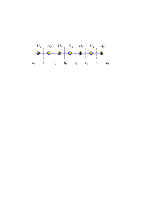
Figure 1: The Dynkin diagram of $\mathfrak{psu}(4|4)$ in the preferred basis.

(for a non-standard parity assignment, which is distinguished by the Bethe ansatz equations [13]). The eight diagonal elements of the supermatrix are depicted as vertical bars (”B” and ”F” stands for the bosonic or fermionic parity). The $l$th node of the Dynkin diagram connects the $l$th bar with the $(l+1)$st. If the eigenvalues have the same parity the node that connects them is bosonic and the diagonal component $A_{ll}$ of the Cartan matrix is equal to $2$ or $-2$. If the parity is opposite, the node is fermionic and $A_{ll}=0$.

The Cartan matrix is not unique for a supergroup [67, 68]. It depends on the parity assignment for rows an columns, and changes non-trivially under their permutation. There is a preferred parity assignment in which the set of integral equations (2.41) can be directly related to the Bethe ansatz equations for the quantum spectrum of the string:

$$(-1)^{|i|}=(+--++--+).$$ (3.8)

This is shown in fig. 1. The associated Cartan basis have the following structure:

$$H_{1}$$

-1 B

-1 -1 F

-1 -1 F

-1 -1 B

-1 -1 B

-1 -1 F

-1 -1 F

-1 B

(3.9)

and the Cartan matrix is

$$A=\begin{pmatrix}&\hphantom{-}1&&&&&\\ \hphantom{-}1&-2&\hphantom{-}1&&&&\\ &\hphantom{-}1&&-1&&&\\ &&-1&\hphantom{-}2&-1&&\\ &&&-1&&\hphantom{-}1&\\ &&&&\hphantom{-}1&-2&\hphantom{-}1\\ &&&&&\hphantom{-}1&\end{pmatrix}.$$ (3.10)

The $\mathbb{Z}_{4}$ automorphism, which defines the coset structure of $PSU(2,2|4)/SO(4,1)\times SO(5)$, acts on the supermatrices of the standard grading $(++++----)$ as [41]:

$$\Omega\circ\begin{pmatrix}A&\Theta\\ \Psi&B\\ \end{pmatrix}=\begin{pmatrix}JA^{t}J&-J\Psi^{t}J\\ J\Theta^{t}J&JB^{t}J\\ \end{pmatrix},\qquad J=\begin{pmatrix}0&-\mathbbm{1}_{2\times 2}\\ \mathbbm{1}_{2\times 2}&0\\ \end{pmatrix}.$$ (3.11)

The action on the diagonal matrices amounts in permutation of their eigenvalues with simultaneous change of the sign:

$$B_{i}\rightarrow-B_{\sigma(i)},\qquad F_{i}\rightarrow-F_{\sigma(i)},$$ (3.12)

where $\sigma=(3412)$. Taking into account that the distinguished basis on fig. 1 is related to the standard one by further permutation of indices, we find that in the distinguished basis $\sigma=(2143)$. From that, and using the explicit form of the Cartan generators (3.9), we can infer how the $\mathbb{Z}_{4}$ generator acts on the Cartan elements and thus compute the matrix $S_{lm}$ defined in (2.35):

$$S=\begin{pmatrix}&&\hphantom{-}1&-1&&&\\ &\hphantom{-}1&&-1&&&\\ \hphantom{-}1&&&-1&&&\\ &&&-1&&&\\ &&&-1&&&\hphantom{-}1\\ &&&-1&&\hphantom{-}1&\\ &&&-1&\hphantom{-}1&&\end{pmatrix}.$$ (3.13)

Next, we should determine vector $\kappa_{l}$, which enters the right-hand-side of the finite-gap equations (2.41) and which must satisfy the conditions (2.38) and (2.42). The eigenvalue equation (2.38) has three linearly independent solutions, one of which is annihilated by the Cartan matrix $A_{lm}$. Adding to $\kappa_{l}$ a zero eigenvector of the Cartan matrix does not change anything, since $\kappa_{l}$ enters the equations in the combination $A_{lk}\kappa_{k}$, and thus we can concentrate on the orthogonal two-dimensional subspace. The null condition (2.42) then has two solutions, $\kappa_{l}\propto(1,2,3,4,3,2,1)$ and $\kappa_{l}\propto(1,0,-1,0,-1,0,1)$. The second solution appears to be the right one, and the classical Bethe equations (2.41) take the following form [25]:

$$2\pi n_{1,i} = \int du({\tt y})\,\frac{\rho_{2}({\tt y})}{u({\tt x})-u({\tt y})}+\int\frac{d{\tt y}}{{\tt y}^{2}}\,\,\frac{\rho_{4}({\tt y})}{{\tt x}-\frac{1}{{\tt y}}}$$

$$2\pi n_{2,i} = \int du({\tt y})\,\frac{\rho_{1}({\tt y})}{u({\tt x})-u({\tt y})}-2-\!\!\!\!\!\!\!\!\;\int du({\tt y})\,\frac{\rho_{2}({\tt y})}{u({\tt x})-u({\tt y})}$$

$$+\int du({\tt y})\,\frac{\rho_{3}({\tt y})}{u({\tt x})-u({\tt y})}$$

$$2\pi n_{3,i} = \int du({\tt y})\,\frac{\rho_{2}({\tt y})}{u({\tt x})-u({\tt y})}-\int d{\tt y}\,\frac{\rho_{4}({\tt y})}{{\tt x}-{\tt y}}$$

$$\frac{2\kappa{\tt x}}{{\tt x}^{2}-1}+2\pi n_{4,i} = \int\frac{d{\tt y}}{{\tt y}^{2}}\,\,\frac{\rho_{1}({\tt y})}{{\tt x}-\frac{1}{{\tt y}}}-\int d{\tt y}\,\frac{\rho_{3}({\tt y})}{{\tt x}-{\tt y}}+2-\!\!\!\!\!\!\!\!\;\int d{\tt y}\,\frac{\rho_{4}({\tt y})}{{\tt x}-{\tt y}}-\int d{\tt y}\,\frac{\rho_{\bar{3}}({\tt y})}{{\tt x}-{\tt y}}$$

$$+\int\frac{d{\tt y}}{{\tt y}^{2}}\,\,\frac{\rho_{\bar{1}}({\tt y})}{{\tt x}-\frac{1}{{\tt y}}}$$

$$2\pi n_{\bar{3},i} = \int du({\tt y})\,\frac{\rho_{\bar{2}}({\tt y})}{u({\tt x})-u({\tt y})}-\int d{\tt y}\,\frac{\rho_{4}({\tt y})}{{\tt x}-{\tt y}}$$

$$2\pi n_{\bar{2},i} = \int du({\tt y})\,\frac{\rho_{\bar{1}}({\tt y})}{u({\tt x})-u({\tt y})}-2-\!\!\!\!\!\!\!\!\;\int du({\tt y})\,\frac{\rho_{\bar{2}}({\tt y})}{u({\tt x})-u({\tt y})}$$

$$+\int du({\tt y})\,\frac{\rho_{\bar{3}}({\tt y})}{u({\tt x})-u({\tt y})}$$

$$2\pi n_{\bar{1},i} = \int du({\tt y})\,\frac{\rho_{\bar{2}}({\tt y})}{u({\tt x})-u({\tt y})}+\int\frac{d{\tt y}}{{\tt y}^{2}}\,\,\frac{\rho_{4}({\tt y})}{{\tt x}-\frac{1}{{\tt y}}}\,.$$ (3.14)

Here $u({\tt x})$ is the Zhukowski variable

$$u({\tt x})={\tt x}+\frac{1}{{\tt x}}\,.$$ (3.15)

In the quantum Bethe equations, the Zhukowski variable plays much more fundamental role than the spectral parameter ${\tt x}$. Here it arises because of the identity

$$d{\tt y}\left(\frac{1}{{\tt x}-{\tt y}}-\frac{1}{{\tt y}^{2}}\,\,\frac{1}{{\tt x}-\frac{1}{{\tt y}}}\right)=\frac{du({\tt y})}{u({\tt x})-u({\tt y})}\,.$$

Once the direct and inversion-symmetry kernels appear with opposite signs, they combine into the simple Hilbert kernel in terms of the Zhukowski variable.

The integral equations are summarized in the diagram in fig. 2.

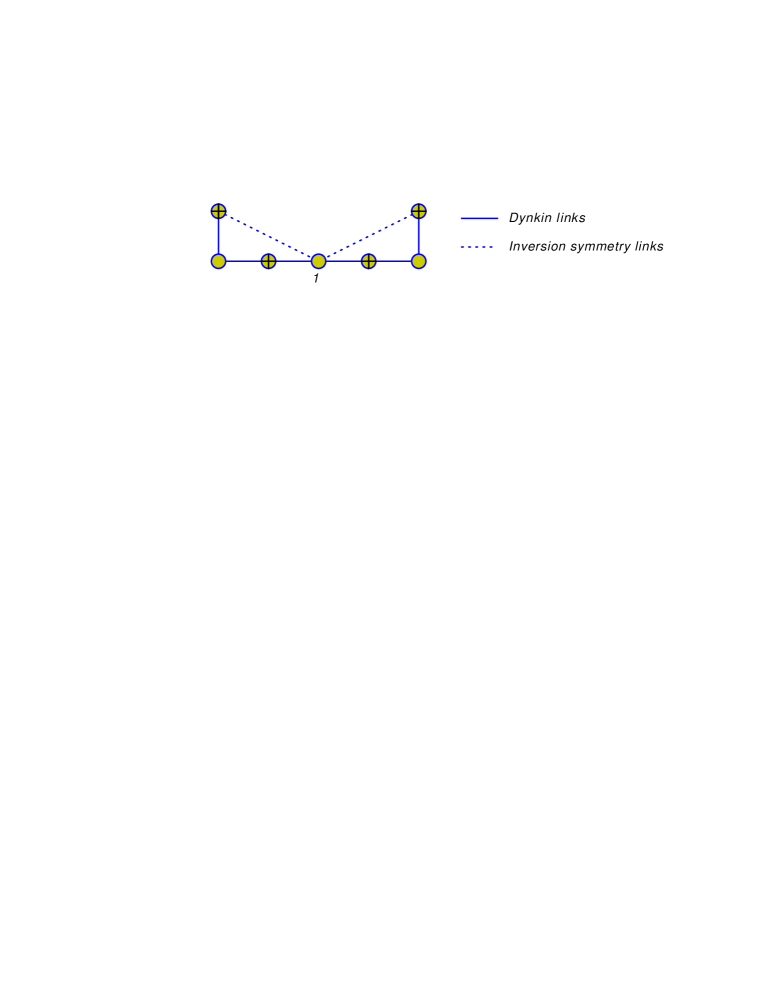
Figure 2: The Dykin diagram for classical Bethe equations in $AdS_{5}\times S^{5}$.

The couplings between various densities mostly follow the structure of the Dynkin diagram of $\mathfrak{psu}(2,2|4)$. Addition interactions arise due to the inversion symmetry. These interactions lead to the extra links in fig. 2 which connect the central node to the ”wrong” fermionic nodes. The central node plays rather distinguished role in the classical Bethe equations (as well as in their quantum counterpart). The source term appears only in the equation for $\rho_{4}$. Closely related to this is the fact that the energy and momentum are computed as moments of the $\rho_{4}({\tt x})$ density:

$$\mathcal{E}-\mathcal{J}=\int d{\tt x}\,\frac{\rho_{4}({\tt x})}{{\tt x}^{2}}$$

$$\mathcal{P}=\int d{\tt x}\,\frac{\rho_{4}({\tt x})}{{\tt x}}\,.$$ (3.16)

Therefore the central node is the only one that carries energy and momentum. Roughly speaking, the normalization of $\rho_{4}$ counts the total number of excited string oscillator modes in a given classical solution. The other nodes of the Dynkin diagram are auxiliary. They determine the flavor structure of the corresponding string state (in which directions the string oscillates), but do not change the energy and momentum.

We will not describe in detail the algebraic curve that solves the integral equations (3.2), see [25, 30]. Basically the structure of the curve follows the Dynkin diagram in fig. 1: the curve is a Riemann surface with eight sheets. Each sheet represents an eigenvalue of the monodromy matrix and is depicted in fig. 1 by a vertical bar. The cuts that connect the sheets carry the densities and are associated to the nodes of the Dynkin diagram. We only considered the densities connecting adjacent sheets, which correspond to the simple roots of the $\mathfrak{psl}(4|4)$ algebra. The cuts going through several sheets are stacks combined from several elementary densities [61, 56].

3.3 Strings on $AdS_{4}\times CP^{3}$

The type IIA string background $AdS_{4}\times CP^{3}$ is dual to $\mathcal{N}=6$ Chern-Simons-matter theory in three dimensions [69], whose superconformal symmetry group is $OSp(6|4)$. The full Green-Schwarz action on $AdS_{4}\times CP^{3}$ is rather complicated [70], but upon partially fixing the kappa-symmetry it reduces to a supercoset sigma-model [42, 43]. The coset, $OSp(6|4)/U(3)\times SO(3,1)$, has $\mathbb{Z}_{4}$ symmetry and therefore is integrable.

The $\mathfrak{osp}(6|4)$ superalgebra can be represented by $(6|4)$ supermatrices:

$$\mathfrak{osp}(6|4)=\left\{\begin{pmatrix}A&\Theta\\ \Psi&B\\ \end{pmatrix}\right|\left.A^{t}=-A,B^{t}=JBJ,\Psi=J\Theta^{t}\right\},\qquad J=\mathbbm{1}\otimes i\sigma^{2}.$$ (3.17)

The Cartan generators can be chosen in the form:

$$H_{l}=\Lambda_{l}\otimes i\sigma^{2},\qquad l=1,\ldots,5,$$ (3.18)

where $\Lambda_{l}$ are diagonal matrices. One should again pick the grading. The preferred choice for constructing the Bethe equations is $(+--++)$, where the pluses correspond to the $\mathfrak{so}(6)$ and minuses to the $\mathfrak{sp}(4)$ subalgebras. The Cartan genrators are

$$\Lambda_{1}$$

-1 B

-1 -1 F

-1 -1 F

-1 -1 -1 B

-1 -1 B

(3.19)

and the Cartan matrix ($A_{lm}=\mathop{\mathrm{Str}}H_{l}H_{m}$) is

$$A=\begin{pmatrix}&\hphantom{-}1&&&\\ \hphantom{-}1&-2&\hphantom{-}1&&\\ &\hphantom{-}1&&-1&-1\\ &&-1&\hphantom{-}2&\\ &&-1&&\hphantom{-}2\\ \end{pmatrix}.$$ (3.20)

The $\mathbb{Z}_{4}$ symmetry acts by conjugation. In the $(+++--)$ grading,

$$\Omega\circ\begin{pmatrix}A&\Theta\\ \Psi&B\\ \end{pmatrix}=\begin{pmatrix}-\hat{J}A\hat{J}&-\hat{J}\Theta K\\ K\Psi\hat{J}&KBK\\ \end{pmatrix},$$ (3.21)

where

$$\hat{J}=\begin{pmatrix}&&&&&\hphantom{-}1\\ &&&&\hphantom{-}1&\\ &&&-1&&\\ &&\hphantom{-}1&&&\\ &-1&&&&\\ -1&&&&&\end{pmatrix},\qquad K=\sigma^{2}\otimes\sigma^{1}.$$ (3.22)

On the matrices of the form (3.18) $\Omega$ acts as

$$\Omega\circ\mathop{\mathrm{diag}}\left(\lambda_{1},\lambda_{2},\lambda_{3},\lambda_{\bar{1}},\lambda_{\bar{2}}\right)\otimes i\sigma^{2}=\left(-\lambda_{3},\lambda_{2},-\lambda_{1},-\lambda_{\bar{2}},-\lambda_{\bar{1}}\right)\otimes i\sigma^{2}.$$ (3.23)

Permutating the indices in order to change the grading to (3.19), we find that the $\mathbb{Z}_{4}$ transformation acts on the eigenvalues of $\Lambda$ as

$$\Omega:B_{1},F_{1},F_{2},B_{2},B_{3}\rightarrow-B_{2},-F_{2},-F_{1},-B_{1},B_{3}.$$ (3.24)

Given the Cartan generators in (3.19), we can now compute the matrix $S$ from (2.35):

$$S=\begin{pmatrix}&&\hphantom{-}1&-1&-1\\ &\hphantom{-}1&&-1&-1\\ \hphantom{-}1&&&-1&-1\\ &&&&-1\\ &&&-1&\end{pmatrix}$$ (3.25)

Now we can compute $\kappa_{l}$ with the help of (2.38) and (2.42). The inversion matrix (3.25) has two eigenvectors with eigenvalue $-1$. The null condition (2.42), evaluated on the linear combination of these eigenvectors, has two linearly independent solutions, $\kappa_{l}\propto(1,2,3,2,2)$ and $\kappa_{l}\propto(1,0,-1,0,0)$. The first solution is unphysical. Substituting the latter solution in the integral equations (2.41), we get [28]

$$2\pi n_{1,i} = \int du({\tt y})\,\frac{\rho_{2}({\tt y})}{u({\tt x})-u({\tt y})}+\int\frac{d{\tt y}}{{\tt y}^{2}}\,\,\frac{\rho_{4}({\tt y})}{{\tt x}-\frac{1}{{\tt y}}}+\int\frac{d{\tt y}}{{\tt y}^{2}}\,\,\frac{\rho_{\bar{4}}({\tt y})}{{\tt x}-\frac{1}{{\tt y}}}$$

$$2\pi n_{2,i} = \int du({\tt y})\,\frac{\rho_{1}({\tt y})}{u({\tt x})-u({\tt y})}-2-\!\!\!\!\!\!\!\!\;\int du({\tt y})\,\frac{\rho_{2}({\tt y})}{u({\tt x})-u({\tt y})}$$

$$+\int du({\tt y})\,\frac{\rho_{3}({\tt y})}{u({\tt x})-u({\tt y})}$$

$$2\pi n_{3,i} = \int du({\tt y})\,\frac{\rho_{2}({\tt y})}{u({\tt x})-u({\tt y})}-\int{d{\tt y}}\,\frac{\rho_{4}({\tt y})}{{\tt x}-{{\tt y}}}-\int{d{\tt y}}\,\frac{\rho_{\bar{4}}({\tt y})}{{\tt x}-{{\tt y}}}$$

$$\frac{\kappa{\tt x}}{{\tt x}^{2}-1}+2\pi n_{4,i} = \int\frac{d{\tt y}}{{\tt y}^{2}}\,\,\frac{\rho_{1}({\tt y})}{{\tt x}-\frac{1}{{\tt y}}}-\int d{\tt y}\,\frac{\rho_{3}({\tt y})}{{\tt x}-{\tt y}}+2-\!\!\!\!\!\!\!\!\;\int d{\tt y}\,\frac{\rho_{4}({\tt y})}{{\tt x}-{\tt y}}-\int\frac{d{\tt y}}{{\tt y}^{2}}\,\,\frac{\rho_{4}({\tt y})}{{\tt x}-\frac{1}{{\tt y}}}$$

$$+\int\frac{d{\tt y}}{{\tt y}^{2}}\,\,\frac{\rho_{\bar{4}}({\tt y})}{{\tt x}-\frac{1}{{\tt y}}}$$

$$\frac{\kappa{\tt x}}{{\tt x}^{2}-1}+2\pi n_{\bar{4},i} = \int\frac{d{\tt y}}{{\tt y}^{2}}\,\,\frac{\rho_{1}({\tt y})}{{\tt x}-\frac{1}{{\tt y}}}-\int d{\tt y}\,\frac{\rho_{3}({\tt y})}{{\tt x}-{\tt y}}+2-\!\!\!\!\!\!\!\!\;\int d{\tt y}\,\frac{\rho_{\bar{4}}({\tt y})}{{\tt x}-{\tt y}}-\int\frac{d{\tt y}}{{\tt y}^{2}}\,\,\frac{\rho_{\bar{4}}({\tt y})}{{\tt x}-\frac{1}{{\tt y}}}$$ (3.26)

$$+\int\frac{d{\tt y}}{{\tt y}^{2}}\,\,\frac{\rho_{4}({\tt y})}{{\tt x}-\frac{1}{{\tt y}}}\,.$$

The equations can be summarized by the Dynkin diagram in fig. 3.

Figure 3: The Dynkin diagram for classical Bethe equations in $AdS_{4}\times CP^{3}$.

The diagram has two momentum-carrying nodes, which are connected with each other by an inversion-symmetry link.

3.4 Strings on $AdS_{3}\times S^{3}$

The Ramond-Ramond backgrounds of the form $AdS_{3}\times S^{3}\times M_{4}$ are dual to two-dimensional superconformal field theories. The extra compact manifold $M_{4}$ is either a $K3$ surface [1, 71] ($T^{4}$ is the simplest possibility) or $S^{3}\times S^{1}$ [72, 73, 74, 75, 76]. These two cases are related, although their superconformal symmetry is different: $PSU(1,1|2)\times PSU(1,1|2)$ for $M_{4}=T^{4}$ or $K3$, and $D(2,1;\alpha)\times D(2,1;\alpha)$ for $M_{4}=S^{3}\times S^{1}$. We first consider the simpler case of $M_{4}=T^{4}$.

The Green-Schwarz string action on $AdS_{3}\times S^{3}$ is a supercoset sigma-model on $PSU(1,1|2)\times PSU(1,1|2)/SU(1,1)\times SU(2)$ [44, 45, 46], which possesses a $\mathbb{Z}_{4}$ symmetry and consequently is integrable [47]. In contradistinction to the previously considered cases, the coset constitutes only part of the geometry and does not contain the $T^{4}$ factor. One may wonder if the $T^{4}$ can at all be coupled to the coset without ruining integrability and supersymmetry. Fortunately, this is possible, because the kappa-symmetry of the 10d Green-Schwarz action on $AdS_{3}\times S^{3}\times T^{4}$ can be fixed in such a way that $T^{4}$ completely decouples [26]. At the classical level one can even treat the coset as a closed sector, but obviously such a truncation is impossible in the quantum theory, at least in any direct sense. Incorporating the $T^{4}$ factor in the quantum integrability framework remains an unresolved problem.

We will derive the finite gap equations for the string on $AdS_{3}\times S^{3}$, completely ignoring the $T^{4}$ factor. The starting point is the Cartan basis (3.6), which for $\mathfrak{psu}(1,1|2)$ in the preferred $(-++-)$ grading takes the form

$$H_{1}$$

-1 F

-1 -1 B

-1 -1 B

-1 F

(3.27)

The Cartan matrix is

$$A=\begin{pmatrix}0&-1&0\\ -1&\hphantom{-}2&-1\\ 0&-1&0\end{pmatrix}.$$ (3.28)

The denominator of the coset is the direct product $PSU(1,1|2)\times PSU(1,1|2)$, with the Cartan matrix

$$A_{\mathfrak{psu}(1,1|2)\oplus\mathfrak{psu}(1,1|2)}=A_{\mathfrak{psu}(1,1|2)}\otimes\mathbbm{1}.$$ (3.29)

The $\mathbbm{Z}_{4}$ symmetry generator of the $PSU(1,1|2)\times PSU(1,1|2)/SU(1,1)\times SU(2)$ coset is a combination of the fermion parity and permutation of the two $\mathfrak{psu}(1,1|2)$ factors

$$\Omega=\begin{pmatrix}0&\mathop{\mathrm{id}}\\ (-1)^{F}&0\\ \end{pmatrix},$$ (3.30)

so that the invariant (denominator) subgroup is the bosonic part of $PSU(1,1|2)$ diagonally embedded into the direct product. On the Grassmann-even generators the $\mathbb{Z}_{4}$ symmetry acts just by a permutation. The $\mathbb{Z}_{4}$ transformations of the Cartan basis are then generated by

$$S=\mathbbm{1}\otimes\sigma^{1}.$$ (3.31)

The solutions of the eigenvalue equation (2.38) are of the form $\kappa\propto v\otimes(1,-1)$. According to (2.42), $v$ should satisfy $v^{t}Av=0$. The null eigenvalue of $A$, $(1,0,-1)$, can be added with arbitrary coefficient. Up to this ambiguity which does not affect the resulting source term in the integral equations, there are two solutions: $v\propto(1,0,1)$ and $v\propto(1,2,1)$. The first solution gives the correct source term in the Bethe equations.

From these data we find [26] (fig. 4):

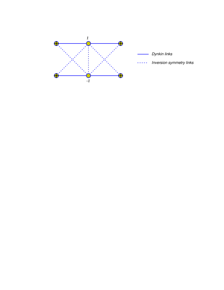
Figure 4: The Dynkin diagram for the $PSU(1,1|2)\times PSU(1,1|2)/SU(1,1)\times SU(2)$ coset.

$$2\pi n_{1,i}^{\pm} = -\int d{\tt y}\,\,\frac{\rho^{\pm}_{2}}{{\tt x}-{\tt y}}+\int\frac{d{\tt y}}{{\tt y}^{2}}\,\,\frac{\rho^{\mp}_{2}}{{\tt x}-\frac{1}{{\tt y}}}$$

$$\pm\frac{2\kappa{\tt x}}{{\tt x}^{2}-1}+2\pi n_{2,i}^{\pm} = -\int d{\tt y}\,\,\frac{\rho^{\pm}_{1}}{{\tt x}-{\tt y}}+2-\!\!\!\!\!\!\!\!\,\int d{\tt y}\,\,\frac{\rho^{\pm}_{2}}{{\tt x}-{\tt y}}-\int d{\tt y}\,\,\frac{\rho^{\pm}_{3}}{{\tt x}-{\tt y}}$$

$$+\int\frac{d{\tt y}}{{\tt y}^{2}}\,\,\frac{\rho^{\mp}_{1}}{{\tt x}-\frac{1}{{\tt y}}}-2\int\frac{d{\tt y}}{{\tt y}^{2}}\,\,\frac{\rho^{\mp}_{2}}{{\tt x}-\frac{1}{{\tt y}}}+\int\frac{d{\tt y}}{{\tt y}^{2}}\,\,\frac{\rho^{\mp}_{3}}{{\tt x}-\frac{1}{{\tt y}}}$$

$$2\pi n_{3,i}^{\pm} = -\int d{\tt y}\,\,\frac{\rho^{\pm}_{2}}{{\tt x}-{\tt y}}+\int\frac{d{\tt y}}{{\tt y}^{2}}\,\,\frac{\rho^{\mp}_{2}}{{\tt x}-\frac{1}{{\tt y}}}$$ (3.32)

The structure of these equations is very similar to the structure of the finite-gap equations for $AdS_{5}\times S^{5}$ and $AdS_{4}\times CP^{3}$. One may then write down the quantum Bethe equations, of which (3.4) is the classical limit, following the analogy with the $AdS_{5}$ and $AdS_{4}$ cases [26]. However, here the finite-gap equations describe only a subset of the degrees of freedom of the string, because the coset constitutes only a part of the geometry. The string fluctuations in $T^{4}$ are describes neither by the finite-gap equations nor by their conjectured quantum counterpart, which thus capture at best a subsector of the full string spectrum on $AdS_{3}\times S^{3}\times T^{4}$.

3.5 Strings on $AdS_{3}\times S^{3}\times S^{3}$

The $AdS_{3}\times S^{3}\times S^{3}\times S^{1}$ background is in many respects similar to $AdS_{3}\times S^{3}\times T^{4}$. The supergroup $PSU(1,1|2)$ gets replaced by $D(2,1;\alpha)$, but the $\mathbbm{Z}_{4}$ symmetry acts as before by eq. (3.30). The supercoset $D(2,1;\alpha)\times D(2,1;\alpha)/SU(1,1)\times SU(2)\times SU(2)$ [26] describes the $AdS_{3}\times S^{3}\times S^{3}$ part of the geometry. The $S^{1}$ factor has to be added by hand. One can recover $AdS_{3}\times S^{3}\times T^{4}$ in the limiting case of $\alpha=0$, when one of the three-spheres blows up to an infinite size and can be recompactified to $T^{3}$. The superalgebra $\mathfrak{d}(2,1;\alpha)$ then reduces to $\mathfrak{psu}(1,1|2)$, up to some Abelian factors. We will not discuss here the case of arbitrary $\alpha$ (see [26]) and will concentrate on another special point, $\alpha=1/2$, when $\mathfrak{d}(2,1;\alpha)$ coincides with the classical Lie superalgebra $\mathfrak{osp}(4|2)$.

The $\mathfrak{osp}$ Cartan basis (3.17), (3.18) for $\mathfrak{osp}(4|2)$ takes the form:

$$\Lambda_{1}$$

-1 F

-1 -1 -1 B

-1 -1 B

(3.33)

The Cartan matrix is

$$A=\begin{pmatrix}\hphantom{-}2&-1&\hphantom{-}0\\ -1&\hphantom{-}0&-1\\ \hphantom{-}0&-1&\hphantom{-}2\end{pmatrix}.$$ (3.34)

As before, the $\mathbb{Z}_{4}$ generator is given by (3.30) and acts on the Cartan generators as in (3.31).

To find the source term in the integral equations we need to solve the conditions (2.38), (2.42). There is an isolated solution $(0,1,0)\otimes(1,-1)$, as well as a one-parametric family $(a,a^{2}+(1-a)^{2},1-a)\otimes(1,-1)$, which is spurious and has to be discarded.

Thus we get for the integral equations:

$$\pm\frac{2\kappa{\tt x}}{{\tt x}^{2}-1}+2\pi n_{1,i}^{\pm} = 2-\!\!\!\!\!\!\!\!\,\int d{\tt y}\,\,\frac{\rho^{\pm}_{1}}{{\tt x}-{\tt y}}-\int d{\tt y}\,\,\frac{\rho^{\pm}_{2}}{{\tt x}-{\tt y}}$$

$$-2\int\frac{d{\tt y}}{{\tt y}^{2}}\,\,\frac{\rho^{\mp}_{1}}{{\tt x}-\frac{1}{{\tt y}}}+\int\frac{d{\tt y}}{{\tt y}^{2}}\,\,\frac{\rho^{\mp}_{2}}{{\tt x}-\frac{1}{{\tt y}}}$$

$$2\pi n_{2,i}^{\pm} = -\int d{\tt y}\,\,\frac{\rho^{\pm}_{1}}{{\tt x}-{\tt y}}-\int d{\tt y}\,\,\frac{\rho^{\pm}_{3}}{{\tt x}-{\tt y}}$$

$$+\int\frac{d{\tt y}}{{\tt y}^{2}}\,\,\frac{\rho^{\mp}_{1}}{{\tt x}-\frac{1}{{\tt y}}}+\int\frac{d{\tt y}}{{\tt y}^{2}}\,\,\frac{\rho^{\mp}_{3}}{{\tt x}-\frac{1}{{\tt y}}}$$

$$\pm\frac{2\kappa{\tt x}}{{\tt x}^{2}-1}+2\pi n_{3,i}^{\pm} = 2-\!\!\!\!\!\!\!\!\,\int d{\tt y}\,\,\frac{\rho^{\pm}_{3}}{{\tt x}-{\tt y}}-\int d{\tt y}\,\,\frac{\rho^{\pm}_{2}}{{\tt x}-{\tt y}}$$ (3.35)

$$-2\int\frac{d{\tt y}}{{\tt y}^{2}}\,\,\frac{\rho^{\mp}_{3}}{{\tt x}-\frac{1}{{\tt y}}}+\int\frac{d{\tt y}}{{\tt y}^{2}}\,\,\frac{\rho^{\mp}_{2}}{{\tt x}-\frac{1}{{\tt y}}}\,.$$

The Dynkin diagram for these equations is shown in fig. 5.

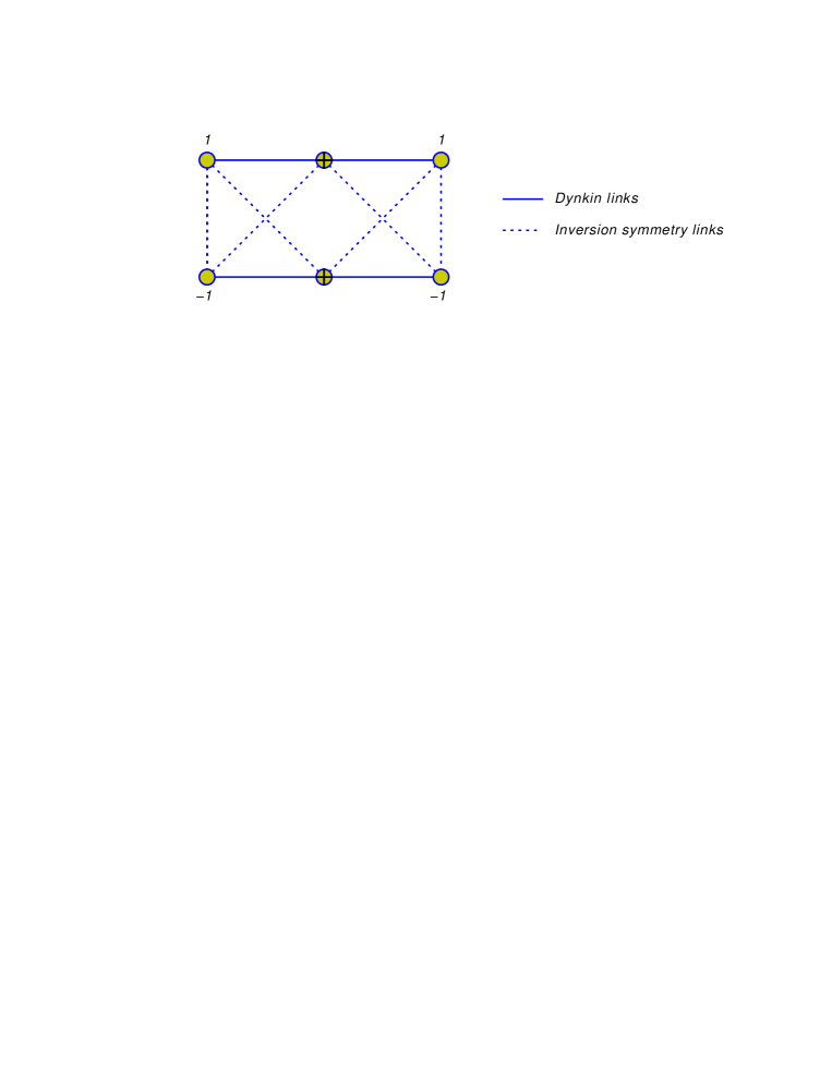
Figure 5: The Dynkin diagram of the classical Bethe equations.

The coset does not include the $S^{1}$ factor and so string fluctuations in the $S^{1}$ directions are not captured by the integral equations. Moreover, in this case the finite-gap equations do not describe the massless degrees of freedom which belong to the coset [26].

3.6 Strings on $AdS_{2}\times S^{2}$

The Green-Schwarz action on $AdS_{2}\times S^{2}$ is described by the $PSU(1,1|2)/U(1)\times U(1)$ coset [48, 36]. In the supermatrix representation of $\mathfrak{su}(1,1|2)$, the $\mathbb{Z}_{4}$ symmetry acts as

$$\Omega\circ\begin{pmatrix}A&\Theta\\ \Psi&B\\ \end{pmatrix}=\begin{pmatrix}\sigma^{2}A\sigma^{2}&i\sigma^{2}\Theta\sigma^{2}\\ -i\sigma^{2}\Psi\sigma^{2}&\sigma^{2}B\sigma^{2}\\ \end{pmatrix},$$ (3.36)

from which we can infer the $\mathbb{Z}_{4}$ transformation of the Cartan elements (3.27):

$$S=\begin{pmatrix}&&-1\\ &-1&\\ -1&&\end{pmatrix}.$$ (3.37)

In the two-dimensional space orthogonal to the zero eigenvalue of the Cartan matrix $(1,0,-1)$ the conditions (2.38) and (2.42) have two solutions: $\kappa_{l}\propto(1,2,1)$ and $\kappa_{l}\propto(1,0,1)$. The former leads to momentum-carrying fermion nodes and has to be discarded. The latter solution gives the following integral equations:

$$2\pi n_{1,i} = \int d{\tt y}\,\rho_{2}({\tt y})\left(\frac{1}{{\tt x}-{\tt y}}+\frac{1}{{\tt y}^{2}}\,\,\frac{1}{{\tt x}-\frac{1}{{\tt y}}}\right)$$

$$\frac{2\kappa{\tt x}}{{\tt x}^{2}-1}+2\pi n_{2,i} = 2-\!\!\!\!\!\!\!\!\;\int d{\tt y}\,\rho_{2}({\tt y})\left(\frac{1}{{\tt x}-{\tt y}}+\frac{1}{{\tt y}^{2}}\,\,\frac{1}{{\tt x}-\frac{1}{{\tt y}}}\right)$$

$$-\int d{\tt y}\,\rho_{1}({\tt y})\left(\frac{1}{{\tt x}-{\tt y}}+\frac{1}{{\tt y}^{2}}\,\,\frac{1}{{\tt x}-\frac{1}{{\tt y}}}\right)$$

$$-\int d{\tt y}\,\rho_{\bar{1}}({\tt y})\left(\frac{1}{{\tt x}-{\tt y}}+\frac{1}{{\tt y}^{2}}\,\,\frac{1}{{\tt x}-\frac{1}{{\tt y}}}\right)$$

$$2\pi n_{\bar{1},i} = \int d{\tt y}\,\rho_{2}({\tt y})\left(\frac{1}{{\tt x}-{\tt y}}+\frac{1}{{\tt y}^{2}}\,\,\frac{1}{{\tt x}-\frac{1}{{\tt y}}}\right).$$ (3.38)

The Dynkin diagram for these equations is shown in fig. 6.

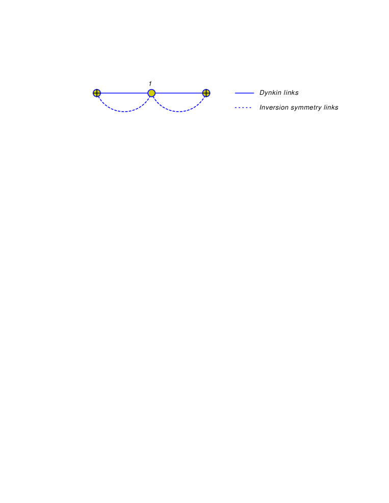
Figure 6: The Dynkin diagram for $AdS_{2}\times S^{2}$.

When the fermionic densities are switched off and there are no stacks, the equation for $\rho_{2}$ reduces to the integral equation for the $O(3)$ sigma-model (3.1). This is not surprising, since the $O(3)$ sigma-model describes a subset of string configurations which move on $S^{2}$ and sit at the centre of $AdS_{2}$.

3.7 $AdS_{2}\times S^{2}\times S^{2}$

The supersymmetric sigma-model on $AdS_{2}\times S^{2}\times S^{2}$ is a $\mathbb{Z}_{4}$ coset $OSp(4|2)/U(1)\times U(1)\times U(1)$ [40] with the $\mathbb{Z}_{4}$ generator

$$\Omega\circ\begin{pmatrix}A&\Theta\\ \Psi&B\\ \end{pmatrix}=\begin{pmatrix}QAQ&iQ\Theta\sigma^{3}\\ -i\sigma^{3}\Psi Q&\sigma^{3}B\sigma^{3}\end{pmatrix},$$ (3.39)

where $Q=\mathop{\mathrm{diag}}(1,-1,1,-1)$. The elements of the Cartan subalgebra (3.18), (3.33) transform just by the reflection of sign:

$$S=-1.$$ (3.40)

The solution of the null condition (2.42) is the same as in sec. 3.5: $\kappa_{l}\propto(0,1,0)$. Combining the Cartan matrix of $\mathfrak{osp}(4|2)$ with the $\mathbb{Z}_{4}$ generator (3.40) and this $\kappa$, we arrive at the following integral equations:

$$\frac{\kappa{\tt x}}{{\tt x}^{2}-1}+2\pi n_{1,i} = 2-\!\!\!\!\!\!\!\!\;\int d{\tt y}\,\rho_{1}({\tt y})\left(\frac{1}{{\tt x}-{\tt y}}+\frac{1}{{\tt y}^{2}}\,\,\frac{1}{{\tt x}-\frac{1}{{\tt y}}}\right)$$

$$-\int d{\tt y}\,\rho_{2}({\tt y})\left(\frac{1}{{\tt x}-{\tt y}}+\frac{1}{{\tt y}^{2}}\,\,\frac{1}{{\tt x}-\frac{1}{{\tt y}}}\right)$$

$$2\pi n_{2,i} = \int d{\tt y}\,\rho_{1}({\tt y})\left(\frac{1}{{\tt x}-{\tt y}}+\frac{1}{{\tt y}^{2}}\,\,\frac{1}{{\tt x}-\frac{1}{{\tt y}}}\right)$$

$$+\int d{\tt y}\,\rho_{\bar{1}}({\tt y})\left(\frac{1}{{\tt x}-{\tt y}}+\frac{1}{{\tt y}^{2}}\,\,\frac{1}{{\tt x}-\frac{1}{{\tt y}}}\right)$$

$$\frac{\kappa{\tt x}}{{\tt x}^{2}-1}+2\pi n_{\bar{1},i} = 2-\!\!\!\!\!\!\!\!\;\int d{\tt y}\,\rho_{\bar{1}}({\tt y})\left(\frac{1}{{\tt x}-{\tt y}}+\frac{1}{{\tt y}^{2}}\,\,\frac{1}{{\tt x}-\frac{1}{{\tt y}}}\right)$$ (3.41)

$$-\int d{\tt y}\,\rho_{2}({\tt y})\left(\frac{1}{{\tt x}-{\tt y}}+\frac{1}{{\tt y}^{2}}\,\,\frac{1}{{\tt x}-\frac{1}{{\tt y}}}\right).$$

The associated Dynkin diagram is shown in fig. 7.

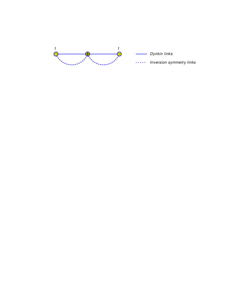
Figure 7: The Dynkin diagram for $AdS_{2}\times S^{2}\times S^{2}$.

3.8 $AdS_{2}\times S^{3}$

The $AdS_{2}\times S^{3}$ coset is $OSp(4|2)/SO(3)\times U(1)$ [40], for which the $\mathbb{Z}_{4}$ generator is given by (3.39) with ${Q}=\mathop{\mathrm{diag}}(-1,1,1,1)$. The $\mathbb{Z}_{4}$ symmetry then acts on the Cartan generators as $\Omega\circ\mathop{\mathrm{diag}}(\lambda_{1},\lambda_{2},\lambda_{3})\otimes i\sigma^{2}=\mathop{\mathrm{diag}}(-\lambda_{1},-\lambda_{2},\lambda_{3})\otimes i\sigma^{2}$. For the Cartan basis (3.33), this gives:

$$S=\begin{pmatrix}&&-1\\ &-1&\\ -1&&\end{pmatrix}.$$ (3.42)

Solving the null condition for the $-1$ eigenvectors of $S$ we find two solutions: the correct solution $\kappa_{l}\propto(0,1,0)$, and the spurious solution $\kappa_{l}\propto(1,1,1)$ which leads to momentum-carrying fermion nodes. The integral equations are

$$\frac{2\kappa{\tt x}}{{\tt x}^{2}-1}+2\pi n_{1,i} = 2-\!\!\!\!\!\!\!\!\;\int d{\tt y}\,\rho_{1}({\tt y})\,\frac{1}{{\tt x}-{\tt y}}-\int d{\tt y}\,\rho_{2}({\tt y})\left(\frac{1}{{\tt x}-{\tt y}}+\frac{1}{{\tt y}^{2}}\,\,\frac{1}{{\tt x}-\frac{1}{{\tt y}}}\right)$$

$$+2\int d{\tt y}\,\rho_{\bar{1}}({\tt y})\,\frac{1}{{\tt y}^{2}}\,\,\frac{1}{{\tt x}-\frac{1}{{\tt y}}}$$

$$2\pi n_{2,i} = \int d{\tt y}\,\rho_{1}({\tt y})\left(\frac{1}{{\tt x}-{\tt y}}+\frac{1}{{\tt y}^{2}}\,\,\frac{1}{{\tt x}-\frac{1}{{\tt y}}}\right)$$

$$+\int d{\tt y}\,\rho_{\bar{1}}({\tt y})\left(\frac{1}{{\tt x}-{\tt y}}+\frac{1}{{\tt y}^{2}}\,\,\frac{1}{{\tt x}-\frac{1}{{\tt y}}}\right)$$

$$\frac{2\kappa{\tt x}}{{\tt x}^{2}-1}+2\pi n_{\bar{1},i} = 2-\!\!\!\!\!\!\!\!\;\int d{\tt y}\,\rho_{\bar{1}}({\tt y})\,\frac{1}{{\tt x}-{\tt y}}-\int d{\tt y}\,\rho_{2}({\tt y})\left(\frac{1}{{\tt x}-{\tt y}}+\frac{1}{{\tt y}^{2}}\,\,\frac{1}{{\tt x}-\frac{1}{{\tt y}}}\right)$$ (3.43)

$$+2\int d{\tt y}\,\rho_{1}({\tt y})\,\frac{1}{{\tt y}^{2}}\,\,\frac{1}{{\tt x}-\frac{1}{{\tt y}}}\,.$$

The Dynkin diagram is shown in fig. 8.

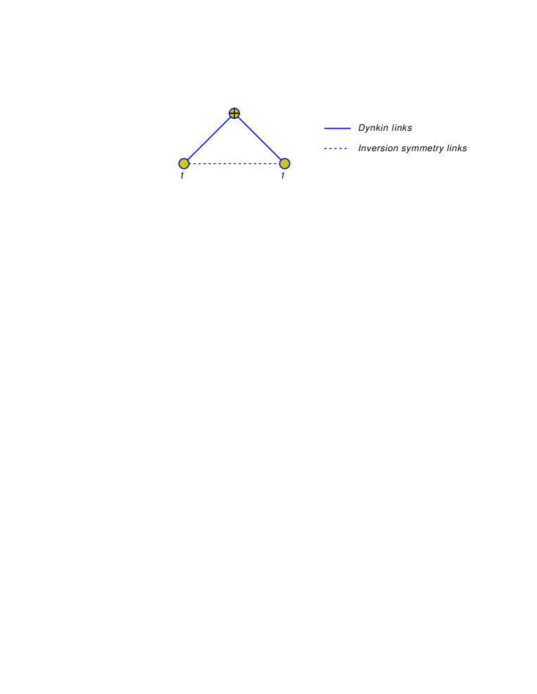
Figure 8: The Dynkin diagram for $AdS_{2}\times S^{3}$.

4 Quantization

The finite-gap integral equations can be regarded as a classical limit of the asymptotic Bethe equations for the quantum spectrum of the string. The first-principles derivation of the Bethe equations requires the knowledge of the exact worldsheet S-matrix [78] in the light-cone gauge. As the experience with the $AdS_{5}$ and $AdS_{4}$ backgrounds demonstrates the exact S-matrices in AdS/CFT [79, 80] are almost uniquely determined by symmetries, unitarity and the crossing condition [81], like in many other integrable models [82, 83] (see [35] for a thorough review of the bootstrap program for strings on $AdS_{5}\times S^{5}$). The diagonalization of the S-matrix for the $n$-particle scattering then yields the Bethe equations. However, a simple set of mnemonic rules allows one to reconstruct the Bethe equations directly from their semiclassical limit, the finite-gap equations of the string sigma-model.

The quantum Bethe equations inherit without change the Dynkin-diagram structure of the finite-gap equations. In the latter, the Dynkin diagram parameterizes the integral kernels, which are of two types: (i) the Hilbert kernel $1/({\tt x}-{\tt y})$ on the Dynkin links (the first term in (2.41)) and (ii) the inversion-symmetry kernel ${\tt y}^{-2}/({\tt x}-1/{\tt y})$ (the second term in (2.41)). Sometimes the two combine to form the Hilbert kernel $1/(u({\tt x})-u({\tt y}))$ in the Zhukowski variables (3.15).

The Zhukowski variable $u$ plays a fundamental role in the quantum Bethe ansatz for $AdS/CFT$, the same as the rapidity plays in the relativistic integrable models. In addition to the spectral parameter ${\tt x}(u)$, given by eq. (3.15), it is convenient to introduce the shifted variables [13]

$${\tt x}^{\pm}+\frac{1}{{\tt x}^{\pm}}=u\pm\frac{i}{2h(\lambda)}\,.$$ (4.1)

In the $AdS_{5}/CFT_{4}$ correspondence, the function $h(\lambda)$ equals to half of the string tension and is related to the ’t Hooft coupling $\lambda$ of $\mathcal{N}=4$ SYM by $h(\lambda)=\sqrt{\lambda}/4\pi$. In other cases $h(\lambda)$ apparently has a more complicated functional dependence on the string tension and scales as $\sqrt{\lambda}$ only in the semiclassical limit $\lambda\rightarrow\infty$. The energy and momentum of a particle with rapidity $u$ are given by

$$\,{\rm e}\,^{\frac{ip}{2h}}=\frac{{\tt x}^{+}}{{\tt x}^{-}}\,\qquad\varepsilon=\frac{i}{2}\left(\frac{1}{{\tt x}^{+}}-\frac{1}{{\tt x}^{-}}\right).$$ (4.2)

The semiclassical limit is the limit of large $h$.

The Bethe equations are generalized periodicity conditions on the multiparticle states, which take into account pairwise scattering. Their generic form is

$$\left(\frac{{\tt x}^{+}(u_{k,l})}{{\tt x}^{-}(u_{k,l})}\right)^{n_{l}L}=\prod_{(j,m)\neq(k,l)}S_{lm}(u_{k,l},u_{j,m}).$$ (4.3)

Here $L$ is the length of the string (some large quantum number related to the angular momentum). The solutions are sets of rapidities $\{u_{k,l}\}$, from which one can determine the energy and the momentum of the corresponding quantum state by summing (4.2) over all momentum-carrying rapidities, those for which $n_{l}\neq 0$. The integral equations of the finite-gap method arise from the thermodynamic limit of the quantum Bethe equations, namely in the limit when the number of rapidities scales with $h\rightarrow\infty$ such that they condense on the cuts in the complex plane and can be characterized by continuous densities

$$\rho_{l}({\tt x})=\frac{1}{h}\sum_{k}\frac{{\tt x}_{k,l}^{2}}{{\tt x}_{k,l}^{2}-1}\,\delta({\tt x}-{\tt x}_{k,l}).$$ (4.4)

At large $h$ the momentum factor in the left-hand side of the Bethe equations expands as

$$\frac{{\tt x}^{+}}{{\tt x}^{-}}\approx 1+\frac{i}{h}\,\,\frac{{\tt x}}{{\tt x}^{2}-1}\,,$$ (4.5)

and produces the force term in the finite-gap equations (2.41).

The scattering factors $S_{lm}({\tt x},{\tt y})$ are determined from the Dynkin diagram, namely from the Cartan matrix $A_{lm}$ and from its product with the inversion-symmetry matrix, $(AS)_{lm}$. The structures that can appear are of four types:

• Bosonic nodes: Each bosonic node of the Dynkin diagram ($A_{ll}=\pm 2$) is associated with a factor

  $$\frac{{\tt x}^{+}-{\tt y}^{-}}{{\tt x}^{-}-{\tt y}^{+}}\,\,\frac{1-\frac{1}{{\tt x}^{+}{\tt y}^{-}}}{1-\frac{1}{{\tt x}^{-}{\tt y}^{+}}}\approx 1+\frac{2i}{h}\left(\frac{{\tt y}^{2}}{{\tt y}^{2}-1}\,\,\frac{1}{{\tt x}-{\tt y}}-\frac{1}{{\tt y}^{2}-1}\,\,\frac{1}{{\tt x}-\frac{1}{{\tt y}}}\right),$$ (4.6)

  which can also be written as

  $$\frac{u-v+\frac{i}{h}}{u-v-\frac{i}{h}}\,,$$ (4.7)

  where $u$ and $v$ are the Zhukowski variables associated with ${\tt x}$ and ${\tt y}$. As one can see from its large-$h$ expansion, this factor contributes $2$ to the Hilbert kernel associated with $A_{ll}$, as it should, but also $-2$ to the inversion kernel associated with $(AS)_{ll}$. When $(AS)_{ll}=A_{ll}$, the two terms in the finite-gap equations combine into a single Zhukowski-type kernel. This is not always the case, and if there is a mismatch, an extra factor should be added to the Bethe equations. This factor is the BES dressing phase [85, 86] $\sigma_{\rm BES}(u,v)$:

  $$\sigma_{\rm BES}(u,v)=\exp\left(-i\sum_{r,s=\pm}rs\,\chi({\tt x}^{r},{\tt y}^{s})\right).$$ (4.8)

  The BES phase is a fairly complicated function of rapidities, which admits the following integral representation [87]:

  $$\chi({\tt x},{\tt y})=\frac{i}{4\pi^{2}}\oint_{|z|=1,|w|=1}\frac{dz\,dw}{({\tt x}-z)({\tt y}-w)}\,\,\ln\frac{\Gamma\left(1+ih\left(z+\frac{1}{z}-w-\frac{1}{w}\right)\right)}{\Gamma\left(1-ih\left(z+\frac{1}{z}-w-\frac{1}{w}\right)\right)}\,.$$ (4.9)

  The BES phase simplifies in the large-$h$ limit when it reduces to the AFS phase [88]:

  $$\chi({\tt x},{\tt y})\approx h({\tt x}-{\tt y})\left(1-\frac{1}{{\tt x}{\tt y}}\right)\ln\left(1-\frac{1}{{\tt x}{\tt y}}\right).$$ (4.10)

  When $h$ is large,

  $${\tt x}^{\pm}={\tt x}\pm\frac{i}{2h}\,\,\frac{{\tt x}^{2}}{{\tt x}^{2}-1}+O\left(\frac{1}{h^{2}}\right),$$ (4.11)

  and

  $$\sum_{sr=\pm}sr\,\chi({\tt x}^{s},{\tt x}^{r})=-\frac{1}{h^{2}}\,\,\frac{{\tt x}^{2}}{{\tt x}^{2}-1}\,\,\frac{{\tt y}^{2}}{{\tt y}^{2}-1}\,\,\frac{\partial^{2}\chi}{\partial{\tt x}\,\partial{\tt y}}+O\left(\frac{1}{h^{4}}\right).$$ (4.12)

  which gives

  $$\sigma_{\rm BES}({\tt x},{\tt y})\approx 1+\frac{i}{h}\left(\frac{1}{{\tt y}^{2}-1}\,\,\frac{1}{{\tt x}-\frac{1}{{\tt y}}}-\frac{1}{{\tt y}^{2}-1}\,\,\frac{{\tt x}}{{\tt x}^{2}-1}\right).$$ (4.13)

  The second term in the brackets, upon integration over ${\tt y}$, shifts the coefficient of the source term in the classical Bethe equations. The first term compensates for the mismatch in the coefficient of the Hilbert and inversion kernels, and thus the BES factor must be raised to the power $A_{ll}-(AS)_{ll}$. For the fermionic nodes, there is no self-scattering term since $A_{ll}=0$, and in all the cases that we have encountered also $(AS)_{ll}=0$.

• Bosonic inversion links: If two different bosonic nodes are connected by the inversion link, we associate to it a BES phase factor $\sigma_{\rm BES}^{-(AS)_{lm}}(u_{k,l},u_{j,m})$. In all the cases when this happens, both nodes are momentum-carrying. This is important for consistency, because the BES phase in the semiclassical limit contributes to the source term in the finite-gap equations, which normally originates from the momentum factor in the Bethe equations. Taking into account the contribution of the BES phase, we can deduce the relationship between the parameters $\kappa_{l}$, that enter the finite-gap equations (2.41), and the length of the string, that enters the quantum Bethe equations (4.3):

  $$A_{lm}\kappa_{m}=\frac{n_{l}L}{h}+A_{lk}\left(\delta_{km}-S_{km}\right)\int d{\tt x}\,\,\frac{\rho_{m}({\tt x})}{{\tt x}^{2}}\,.$$ (4.14)

  Another special property of the Dynkin diagrams that come out of the finite-gap integration procedure is that bosonic and fermionic nodes alternate, such that the same-parity nodes are never connected by normal Dynkin links.

• Dynkin boson-fermion links: A normal Dynkin link between a bosonic and fermionic node is associated with a factor

  $$\frac{{\tt x}-{\tt y}^{+}}{{\tt x}-{\tt y}^{-}}\approx 1-\frac{i}{h}\,\,\frac{{\tt y}^{2}}{{\tt y}^{2}-1}\,\,\frac{1}{{\tt x}-{\tt y}}\,,$$ (4.15)

  where ${\tt x}$ is the fermion spectral parameter and ${\tt y}$ is the boson one. This factor appears in the equation on the fermionic node. In the bosonic-node equation ${\tt x}$ and ${\tt y}$ are interchanged.

• Inversion boson-fermion links: The inversion links that connect momentum-carrying bosonic nodes with the ”wrong” fermionic nodes are associated with a factor

  $$\frac{1-\frac{1}{{\tt x}{\tt y}^{+}}}{1-\frac{1}{{\tt x}{\tt y}^{-}}}\approx 1+\frac{i}{h}\,\,\frac{1}{{\tt y}^{2}-1}\,\,\frac{1}{x-\frac{1}{{\tt y}}}\,.$$ (4.16)

  In the equation on the bosonic node ${\tt x}$ and ${\tt y}$ are again interchanged.

This way one can easily reconstruct the Bethe equations for $AdS_{5}\times S^{5}$ [13] from the Dynkin diagram 2; the Bethe equations for $AdS_{4}\times CP^{3}$ [89] from the diagram 3, and the conjectured Bethe equations for $AdS_{3}\times S^{3}$ or $AdS_{3}\times S^{3}\times S^{3}$ [26] from the diagrams 4 and 5.

Acknowledgments

This work was supported in part by the Swedish Research Council under the contract 621-2007-4177, in part by the ANF-a grant 09-02-91005, and in part by the grant for support of scientific schools NSH-3036.2008.2.

References

- [1] J. M. Maldacena, “The large N limit of superconformal field theories and supergravity”, Adv. Theor. Math. Phys. 2, 231 (1998), hep-th/9711200.
- [2] S. S. Gubser, I. R. Klebanov and A. M. Polyakov, “Gauge theory correlators from non-critical string theory”, Phys. Lett. B428, 105 (1998), hep-th/9802109.
- [3] E. Witten, “Anti-de Sitter space and holography”, Adv. Theor. Math. Phys. 2, 253 (1998), hep-th/9802150.
- [4] I. Bena, J. Polchinski and R. Roiban, “Hidden symmetries of the superstring”, Phys. Rev. D69, 046002 (2004), hep-th/0305116.
- [5] L. D. Faddeev and L. A. Takhtajan, “Hamiltonian methods in the theory of solitons”, Springer (1987), Berlin, Germany, 592p, Springer Series In Soviet Mathematics.
- [6] D. E. Berenstein, J. M. Maldacena and H. S. Nastase, “Strings in flat space and pp waves from N = 4 super Yang Mills”, JHEP 0204, 013 (2002), hep-th/0202021.
- [7] S. S. Gubser, I. R. Klebanov and A. M. Polyakov, “A semi-classical limit of the gauge/string correspondence”, Nucl. Phys. B636, 99 (2002), hep-th/0204051.
- [8] S. Frolov and A. A. Tseytlin, “Multi-spin string solutions in ”, Nucl. Phys. B668, 77 (2003), hep-th/0304255.
- [9] A. A. Tseytlin, “Spinning strings and AdS/CFT duality”, hep-th/0311139.
- [10] J. Plefka, “Spinning strings and integrable spin chains in the AdS/CFT correspondence”, Living Rev. Rel. 8, 9 (2005), hep-th/0507136.
- [11] S. Novikov, S. V. Manakov, L. P. Pitaevsky and V. E. Zakharov, “Theory of solitons. the inverse scattering method”, Consultants Bureau (1984), New York, USA, 276p, Contemporary Soviet Mathematics.
- [12] V. A. Kazakov, A. Marshakov, J. A. Minahan and K. Zarembo, “Classical/quantum integrability in AdS/CFT”, JHEP 0405, 024 (2004), hep-th/0402207.
- [13] N. Beisert and M. Staudacher, “Long-range Bethe ansaetze for gauge theory and strings”, Nucl. Phys. B727, 1 (2005), hep-th/0504190.
- [14] N. Gromov, V. Kazakov and P. Vieira, “Exact Spectrum of Anomalous Dimensions of Planar N=4 Supersymmetric Yang-Mills Theory”, Phys. Rev. Lett. 103, 131601 (2009), 0901.3753.
- [15] D. Bombardelli, D. Fioravanti and R. Tateo, “Thermodynamic Bethe Ansatz for planar AdS/CFT: a proposal”, J. Phys. A42, 375401 (2009), 0902.3930.
- [16] N. Gromov, V. Kazakov, A. Kozak and P. Vieira, “Exact Spectrum of Anomalous Dimensions of Planar N = 4 Supersymmetric Yang-Mills Theory: TBA and excited states”, Lett. Math. Phys. 91, 265 (2010), 0902.4458.
- [17] G. Arutyunov and S. Frolov, “Thermodynamic Bethe Ansatz for the Mirror Model”, JHEP 0905, 068 (2009), 0903.0141.
- [18] D. Bombardelli, D. Fioravanti and R. Tateo, “TBA and Y-system for planar ”, Nucl. Phys. B834, 543 (2010), 0912.4715.
- [19] N. Gromov and F. Levkovich-Maslyuk, “Y-system, TBA and Quasi-Classical Strings in ”, 0912.4911.
- [20] N. Gromov, “Y-system and Quasi-Classical Strings”, JHEP 1001, 112 (2010), 0910.3608.
- [21] N. Gromov, V. Kazakov and Z. Tsuboi, “ Character of Quasiclassical AdS/CFT”, 1002.3981.
- [22] L. F. Alday and J. Maldacena, “Null polygonal Wilson loops and minimal surfaces in Anti- de-Sitter space”, JHEP 0911, 082 (2009), 0904.0663.
- [23] L. F. Alday, D. Gaiotto and J. Maldacena, “Thermodynamic Bubble Ansatz”, 0911.4708.
- [24] L. F. Alday, J. Maldacena, A. Sever and P. Vieira, “Y-system for Scattering Amplitudes”, 1002.2459.
- [25] N. Beisert, V. A. Kazakov, K. Sakai and K. Zarembo, “The algebraic curve of classical superstrings on ”, Commun. Math. Phys. 263, 659 (2006), hep-th/0502226.
- [26] A. Babichenko, B. Stefanski and K. Zarembo, “Integrability and the correspondence”, JHEP 1003, 058 (2010), 0912.1723.
- [27] N. Beisert, V. A. Kazakov and K. Sakai, “Algebraic curve for the SO(6) sector of AdS/CFT”, Commun. Math. Phys. 263, 611 (2006), hep-th/0410253.
- [28] N. Gromov and P. Vieira, “The algebraic curve”, JHEP 0902, 040 (2009), 0807.0437.
- [29] K. Zarembo, “Semiclassical Bethe ansatz and AdS/CFT”, Comptes Rendus Physique 5, 1081 (2004), hep-th/0411191.
- [30] N. Gromov, “Integrability in AdS/CFT correspondence: quasi-classical analysis”, J. Phys. A: Math. Theor 42, 1 (2009).
- [31] R. R. Metsaev and A. A. Tseytlin, “Type IIB superstring action in background”, Nucl. Phys. B533, 109 (1998), hep-th/9805028.
- [32] H. Eichenherr and M. Forger, “On the Dual Symmetry of the Nonlinear Sigma Models”, Nucl. Phys. B155, 381 (1979).
- [33] L. D. Faddeev and N. Y. Reshetikhin, “Integrability of the principal chiral field model in (1+1)-dimension”, Ann. Phys. 167, 227 (1986).
- [34] M. B. Green and J. H. Schwarz, “Covariant Description of Superstrings”, Phys. Lett. B136, 367 (1984).
- [35] G. Arutyunov and S. Frolov, “Foundations of the Superstring. Part I”, J. Phys. A: Math. Theor 42, 1 (2009), 0901.4937.
- [36] N. Berkovits, M. Bershadsky, T. Hauer, S. Zhukov and B. Zwiebach, “Superstring theory on as a coset supermanifold”, Nucl. Phys. B567, 61 (2000), hep-th/9907200.
- [37] R. Roiban and W. Siegel, “Superstrings on supertwistor space”, JHEP 0011, 024 (2000), hep-th/0010104.
- [38] A. M. Polyakov, “Conformal fixed points of unidentified gauge theories”, Mod. Phys. Lett. A19, 1649 (2004), hep-th/0405106.
- [39] I. Adam, A. Dekel, L. Mazzucato and Y. Oz, “Integrability of type II superstrings on Ramond-Ramond backgrounds in various dimensions”, JHEP 0706, 085 (2007), hep-th/0702083.
- [40] K. Zarembo, “Strings on Semisymmetric Superspaces”, 1003.0465.
- [41] V. V. Serganova, “Classification of real simple Lie superalgebras and symmetric superspaces”, Funct. Anal. Appl. 17, 200 (1983).
- [42] G. Arutyunov and S. Frolov, “Superstrings on as a Coset Sigma-model”, JHEP 0809, 129 (2008), 0806.4940.
- [43] j. Stefański, B., “Green-Schwarz action for Type IIA strings on ”, Nucl. Phys. B808, 80 (2009), 0806.4948.
- [44] J. Rahmfeld and A. Rajaraman, “The GS string action on with Ramond-Ramond charge”, Phys. Rev. D60, 064014 (1999), hep-th/9809164.
- [45] J. Park and S.-J. Rey, “Green-Schwarz superstring on ”, JHEP 9901, 001 (1999), hep-th/9812062.
- [46] R. R. Metsaev and A. A. Tseytlin, “Superparticle and superstring in Ramond-Ramond background in light-cone gauge”, J. Math. Phys. 42, 2987 (2001), hep-th/0011191.
- [47] B. Chen, Y.-L. He, P. Zhang and X.-C. Song, “Flat currents of the Green-Schwarz superstrings in and backgrounds”, Phys. Rev. D71, 086007 (2005), hep-th/0503089.
- [48] J.-G. Zhou, “Super 0-brane and GS superstring actions on ”, Nucl. Phys. B559, 92 (1999), hep-th/9906013.
- [49] H. L. Verlinde, “Superstrings on and superconformal matrix quantum mechanics”, hep-th/0403024.
- [50] C. A. S. Young, “Non-local charges, gradings and coset space actions”, Phys. Lett. B632, 559 (2006), hep-th/0503008.
- [51] V. A. Kazakov and K. Zarembo, “Classical/quantum integrability in non-compact sector of AdS/CFT”, JHEP 0410, 060 (2004), hep-th/0410105.
- [52] S. Schafer-Nameki, “The algebraic curve of 1-loop planar N = 4 SYM”, Nucl. Phys. B714, 3 (2005), hep-th/0412254.
- [53] N. Dorey and B. Vicedo, “On the dynamics of finite-gap solutions in classical string theory”, JHEP 0607, 014 (2006), hep-th/0601194.
- [54] N. Dorey and B. Vicedo, “A symplectic structure for string theory on integrable backgrounds”, JHEP 0703, 045 (2007), hep-th/0606287.
- [55] J. R. David and B. Sahoo, “S-matrix for magnons in the D1-D5 system”, 1005.0501.
- [56] N. Gromov and P. Vieira, “Complete 1-loop test of AdS/CFT”, JHEP 0804, 046 (2008), 0709.3487.
- [57] N. Gromov, S. Schafer-Nameki and P. Vieira, “Efficient precision quantization in AdS/CFT”, JHEP 0812, 013 (2008), 0807.4752.
- [58] B. Vicedo, “Semiclassical Quantisation of Finite-Gap Strings”, JHEP 0806, 086 (2008), 0803.1605.
- [59] V. K. Dobrev and V. B. Petkova, “Group Theoretical Approach To Extended Conformal Supersymmetry: Function Space Realizations And Invariant Differential Operators”, Fortschr. Phys. 35, 537 (1987).
- [60] I. Penkov and V. Serganova, “Representations of classical Lie superalgebras of type I”, Indag. Math. N.S.3(4), 419 (1992).
- [61] N. Beisert, V. A. Kazakov, K. Sakai and K. Zarembo, “Complete spectrum of long operators in N = 4 SYM at one loop”, JHEP 0507, 030 (2005), hep-th/0503200.
- [62] B. Sutherland, “Low-Lying Eigenstates of the One-Dimensional Heisenberg Ferromagnet for any Magnetization and Momentum”, Phys. Rev. Lett. 74, 816 (1995).
- [63] A. Dhar and B. S. Shastry, “Bloch Walls and Macroscopic String States in Bethe’s Solution of the Heisenberg Ferromagnetic Linear Chain”, Phys. Rev. Lett. 85, 2813 (2000).
- [64] N. Beisert, J. A. Minahan, M. Staudacher and K. Zarembo, “Stringing spins and spinning strings”, JHEP 0309, 010 (2003), hep-th/0306139.
- [65] N. Gromov, V. Kazakov, K. Sakai and P. Vieira, “Strings as multi-particle states of quantum sigma- models”, Nucl. Phys. B764, 15 (2007), hep-th/0603043.
- [66] N. Gromov, V. Kazakov and P. Vieira, “Classical limit of quantum sigma-models from Bethe ansatz”, PoS SOLVAY, 005 (2006), hep-th/0703137.
- [67] V. G. Kac, “A Sketch of Lie Superalgebra Theory”, Commun. Math. Phys. 53, 31 (1977).
- [68] L. Frappat, P. Sorba and A. Sciarrino, “Dictionary on Lie superalgebras”, hep-th/9607161.
- [69] O. Aharony, O. Bergman, D. L. Jafferis and J. Maldacena, “N=6 superconformal Chern-Simons-matter theories, M2-branes and their gravity duals”, JHEP 0810, 091 (2008), 0806.1218.
- [70] J. Gomis, D. Sorokin and L. Wulff, “The complete superspace for the type IIA superstring and D-branes”, JHEP 0903, 015 (2009), 0811.1566.
- [71] N. Berkovits, C. Vafa and E. Witten, “Conformal field theory of AdS background with Ramond-Ramond flux”, JHEP 9903, 018 (1999), hep-th/9902098.
- [72] S. Elitzur, O. Feinerman, A. Giveon and D. Tsabar, “String theory on ”, Phys. Lett. B449, 180 (1999), hep-th/9811245.
- [73] P. M. Cowdall and P. K. Townsend, “Gauged supergravity vacua from intersecting branes”, Phys. Lett. B429, 281 (1998), hep-th/9801165.
- [74] J. P. Gauntlett, R. C. Myers and P. K. Townsend, “Supersymmetry of rotating branes”, Phys. Rev. D59, 025001 (1999), hep-th/9809065.
- [75] H. J. Boonstra, B. Peeters and K. Skenderis, “Brane intersections, anti-de Sitter spacetimes and dual superconformal theories”, Nucl. Phys. B533, 127 (1998), hep-th/9803231.
- [76] S. Gukov, E. Martinec, G. W. Moore and A. Strominger, “The search for a holographic dual to ”, Adv. Theor. Math. Phys. 9, 435 (2005), hep-th/0403090.
- [77] I. Pesando, “The GS type IIB superstring action on ”, JHEP 9902, 007 (1999), hep-th/9809145.
- [78] M. Staudacher, “The factorized S-matrix of CFT/AdS”, JHEP 0505, 054 (2005), hep-th/0412188.
- [79] N. Beisert, “The dynamic S-matrix”, Adv. Theor. Math. Phys. 12, 945 (2008), hep-th/0511082.
- [80] C. Ahn and R. I. Nepomechie, “N=6 super Chern-Simons theory S-matrix and all-loop Bethe ansatz equations”, JHEP 0809, 010 (2008), 0807.1924.
- [81] R. A. Janik, “The superstring worldsheet S-matrix and crossing symmetry”, Phys. Rev. D73, 086006 (2006), hep-th/0603038.
- [82] A. B. Zamolodchikov and A. B. Zamolodchikov, “Factorized S-matrices in two dimensions as the exact solutions of certain relativistic quantum field models”, Annals Phys. 120, 253 (1979).
- [83] P. Dorey, “Exact S matrices”, hep-th/9810026.
- [84] E. Ogievetsky and P. Wiegmann, “Factorized S matrix and the Bethe ansatz for simple Lie groups”, Phys. Lett. B168, 360 (1986).
- [85] N. Beisert, B. Eden and M. Staudacher, “Transcendentality and crossing”, J. Stat. Mech. 0701, P021 (2007), hep-th/0610251.
- [86] N. Beisert, R. Hernandez and E. Lopez, “A crossing-symmetric phase for strings”, JHEP 0611, 070 (2006), hep-th/0609044.
- [87] N. Dorey, D. M. Hofman and J. M. Maldacena, “On the singularities of the magnon S-matrix”, Phys. Rev. D76, 025011 (2007), hep-th/0703104.
- [88] G. Arutyunov, S. Frolov and M. Staudacher, “Bethe ansatz for quantum strings”, JHEP 0410, 016 (2004), hep-th/0406256.
- [89] N. Gromov and P. Vieira, “The all loop Bethe ansatz”, JHEP 0901, 016 (2009), 0807.0777.