Probing Nearby CR Accelerators and ISM Turbulence with Milagro Hot Spots

Abstract

Both the acceleration of cosmic rays (CR) in supernova remnant shocks and their subsequent propagation through the random magnetic field of the Galaxy deem to result in an almost isotropic CR spectrum. Yet the MILAGRO TeV observatory discovered a sharp ($\sim 10^{\circ})$ arrival anisotropy of CR nuclei. We suggest a mechanism for producing a weak and narrow CR beam which operates en route to the observer. The key assumption is that CRs are scattered by a strongly anisotropic Alfven wave spectrum formed by the turbulent cascade across the local field direction. The strongest pitch-angle scattering occurs for particles moving almost precisely along the field line. Partly because this direction is also the direction of minimum of the large scale CR angular distribution, the enhanced scattering results in a weak but narrow particle excess. The width, the fractional excess and the maximum momentum of the beam are calculated from a systematic transport theory depending on a single scale $l$ which can be associated with the longest Alfven wave, efficiently scattering the beam. The best match to all the three characteristics of the beam is achieved at $l\sim 1$pc. The distance to a possible source of the beam is estimated to be within a few 100pc. Possible approaches to determination of the scale $l$ from the characteristics of the source are discussed. Alternative scenarios of drawing the beam from the galactic CR background are considered. The beam related large scale anisotropic CR component is found to be energy independent which is also consistent with the observations.

1 Introduction

The MILAGRO TeV observatory recently discovered collimated beams dominated by hadronic cosmic rays (CR) with a narrow ($\sim 10^{\circ}$) angular distribution in the 10 TeV energy range (Abdo et al., 2008). This is surprising, since most of the CR acceleration and propagation models predict only a weak, large scale anisotropy. The acceleration models are based on the diffusive shock acceleration (DSA) mechanism, widely believed to generate galactic CRs in supernova remnant shocks (SNR). The corner stone of the DSA is a rapid pitch-angle scattering of CRs by self-generated Alfven waves in the shock vicinity. An enhanced scattering isotropizes particle distributions. Moreover, when the shock releases the accelerated particles into the interstellar medium (ISM), they continue to scatter by the ISM turbulence. Even though this scattering occurs at a significantly lower rate, all sharp anisotropies carried over from the accelerator or created otherwise, should be erased during the long ($\mathrel{\mathchoice{\vbox{\offinterlineskip\halign{\hfil\(\displaystyle#\)\hfil\cr$\displaystyle>$\cr$\displaystyle\sim$\cr}}}{\vbox{\offinterlineskip\halign{\hfil\(\textstyle#\)\hfil\cr$\textstyle>$\cr$\textstyle\sim$\cr}}}{\vbox{\offinterlineskip\halign{\hfil\(\scriptstyle#\)\hfil\cr$\scriptstyle>$\cr$\scriptstyle\sim$\cr}}}{\vbox{\offinterlineskip\halign{\hfil\(\scriptscriptstyle#\)\hfil\cr$\scriptscriptstyle>$\cr$\scriptscriptstyle\sim$\cr}}}}$100 pc) travel of the CRs from any hypothetical nearby SNR to the observer. Yet, the astounding sharp beaming effect is argued to be genuine.

Focusing on relatively distant accelerators (such as nearby SNRs) and long-distance propagation effects as a possible cause of the MILAGRO beam(s), we do not consider ’local’ scenarios that have already been discussed and largely rejected by Drury & Aharonian (2008) and Salvati & Sacco (2008). As for the remote accelerator with subsequent propagation effects, some of them have also been suggested in the above publications. In particular, Salvati & Sacco (2008) associate the observed CR beam with the Geminga pulsar. However, Drury & Aharonian (2008) argue that this does not explain namely the sharp collimation, and suggest a magnetic nozzle as such a collimation device. The magnetic nozzle scenario, however, poses a rather strong constraint on the nozzle mirror ratio ($B_{max}/B_{min}\sim\vartheta^{-2}\gg 1,$ where $\vartheta$ is the beam angular width). The advantage of this scenario is that the beam density is equal to the difference between the isotropic components of CRs on each side of the mirror (by linearity of the transport equation). Since the Milagro beam is very weak ($\sim 10^{-4}$ of the CR density), this is a very mild requirement on the CR enhancement on the far side of the mirror. It is also true that the existence of a magnetic mirror of that strength cannot be warranted or denied on rational ground. It should be noted that any anisotropic distribution may become vulnerable to self-spreading in pitch angle. As pointed out by Drury & Aharonian (2008), however, the isotropic CR background should produce a stabilizing effect against the beam self-spreading. We will quantify the CR stabilization in Sec.4.4 required for both the collimation mechanism suggested in the present paper and for the magnetic nozzle hypothesis.

In this paper we suggest a novel mechanism for producing a narrow CR beam. It is based on the strong anisotropy of the MHD turbulence in the ISM. Such anisotropy is expected when the turbulence is driven at a long (outer) scale, but unlike the isotropic Kolmogorov cascade, the incompressible MHD cascade is directed perpendicularly to the magnetic field in the wave vector space. This was shown by Goldreich & Sridhar (1995) (GS) (see also Sridhar & Goldreich 1994 and Goldreich & Sridhar 1997) and confirmed by numerical simulations ( e.g., Cho & Vishniac 2000; Maron & Goldreich 2001; Beresnyak & Lazarian 2009). The cascade proceeds to $k_{\perp}r_{g}\left(p\right)\gg 1$ in the perpendicular wave number direction for the protons with the gyro-radii $r_{g}\sim 10^{16}$cm, typical for the particles of the MILAGRO beam energies $pc\sim 10$TeV and the ISM magnetic field of a few $\mu G$. Contrary to the $k_{\perp}$ direction the spectrum spreading in $k_{\parallel}$ is suppressed, so that $k_{\parallel}\sim k_{\perp}^{2/3}l^{-1/3}\ll k_{\perp}$, where $l$ is the outer scale.

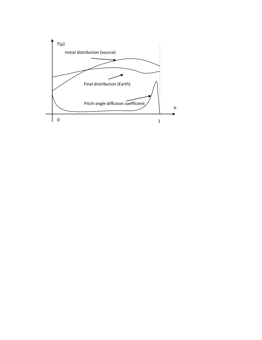
Figure 1: Schematic representation of initial and final pitch-angle distributions and that of the diffusion coefficient $D_{\mu\mu}\left(\mu\right)$.

As is known from the wave-particle interaction in plasmas, the scattering of particles with the Larmor radius exceeding the wave length in the perpendicular direction, $k_{\perp}r_{g}\gg 1$ is strongly suppressed, since such particles suffer a rapidly changing electromagnetic force. Specifically, the CR scattering by the GS anisotropic spectrum was investigated in a number of publications (Chandran 2000; Yan & Lazarian 2002). What is important for the purposes of this paper is that the pitch-angle scattering rate is peaked at $\left|\mu\right|=\left|\cos\vartheta\right|\approx 1$, i.e., for particles moving along the field line, since for these particles $k_{\perp}r_{g}\left(p_{\perp}\right)\mathrel{\mathchoice{\vbox{\offinterlineskip\halign{\hfil\(\displaystyle#\)\hfil\cr$\displaystyle<$\cr$\displaystyle\sim$\cr}}}{\vbox{\offinterlineskip\halign{\hfil\(\textstyle#\)\hfil\cr$\textstyle<$\cr$\textstyle\sim$\cr}}}{\vbox{\offinterlineskip\halign{\hfil\(\scriptstyle#\)\hfil\cr$\scriptstyle<$\cr$\scriptstyle\sim$\cr}}}{\vbox{\offinterlineskip\halign{\hfil\(\scriptscriptstyle#\)\hfil\cr$\scriptscriptstyle<$\cr$\scriptscriptstyle\sim$\cr}}}}1$. Only particles with such small $p_{\perp}$, i.e., with pitch angles within $\sin^{2}\vartheta\mathrel{\mathchoice{\vbox{\offinterlineskip\halign{\hfil\(\displaystyle#\)\hfil\cr$\displaystyle<$\cr$\displaystyle\sim$\cr}}}{\vbox{\offinterlineskip\halign{\hfil\(\textstyle#\)\hfil\cr$\textstyle<$\cr$\textstyle\sim$\cr}}}{\vbox{\offinterlineskip\halign{\hfil\(\scriptstyle#\)\hfil\cr$\scriptstyle<$\cr$\scriptstyle\sim$\cr}}}{\vbox{\offinterlineskip\halign{\hfil\(\scriptscriptstyle#\)\hfil\cr$\scriptscriptstyle<$\cr$\scriptscriptstyle\sim$\cr}}}}\epsilon\ll 1$ are scattered efficiently. Looking at this problem mathematically, a peaked diffusion coefficient $D\left(\mu\right)$ does not necessarily result in a peaked particle distribution $f\left(\mu\right)$. Indeed, the time-asymptotic solution of the diffusion equation with zero flux through the boundary is a flat distribution even if the diffusion coefficient is not constant. Nevertheless, consider the particle diffusion in pitch angle on an intermediate time-scale, i.e., when anisotropy is erased within the strong peak of the diffusion coefficient $D\left(\mu\right)$, but is present in the region where $D\left(\mu\right)$ is much smaller. The dominant eigenfunction of the scattering operator has a relatively broad minimum at $\mu=1$, i.e., where $D$ is sharply peaked. Now, the enhanced scattering fills up the very bottom of this minimum which appears as a narrow excess, Fig.1. In the context of a classical Lorentz gas relaxation problem (Gurevich, 1961; Kruskal & Bernstein, 1964), this is clearly a transient effect associated with an incomplete decay of the anisotropic part of the pitch-angle distribution. Note that the difference with the Lorenz gas problem is in the sharply peaked $D\left(\mu\right)$. In addition, our problem is a problem in $z$, which is the spatial coordinate (rather than time) along a magnetic flux tube that connects the CR source with the Earth.

The demonstration of this phenomenon, facilitated and obscured at the same time by the fact that the peak region $\left|\sin\vartheta\right|\ll 1$ contains the singular points of particle pitch-angle diffusion operator at $\sin\vartheta=0$, will be the main subject of the present paper.

Before we tackle this problem, we briefly discuss in the next section how narrow the CR angular distribution can be as it leaks from a hypothetical nearby SNR accelerator, magnetically connected with the heliosphere. This, or some other moderately anisotropic distribution of CRs, created by a recent SNR explosion, will be subjected in Sec.3 to the pitch-angle scattering analysis and to the propagation analysis in Sec.4. Next, in Sec.4.4 we determine the maximum energy of the beam beyond which it must spread on self-generated Alfven waves. Sec.5 deals with the relation between the beam maximum energy and the distance to its possible source. We conclude with a brief discussion of the results and of what the fascinating MILAGRO findings can possibly tell about a nearby accelerator and the structure of ISM turbulence.

2 Angular distribution of Diffusively accelerated particles

To estimate anisotropy of CRs escaping from a SNR accelerator, we first briefly review the DSA mechanism and its possible modifications that can enhance the CR anisotropy. Within this mechanism particles gain energy by scattering upstream of the shock and back downstream repeatedly. The scattering is supported by strong MHD waves unstably driven by the accelerated particles themselves. In the early phase of acceleration an ion-cyclotron instability dominates. It is driven by a weak pitch-angle anisotropy of particle distribution. It is reasonable to assume, however, that a small fraction of particles that reach sufficiently high energies can diffuse to the distant part of the turbulent shock precursor where their self-confinement becomes inefficient. In this way a somewhat artificial notion of the ’free escape boundary’ (FEB) was introduced, particularly in Monte Carlo numerical schemes (Ellison et al., 1996) and other analytical and numerical studies (Caprioli et al., 2009; Reville et al., 2009). Particle escape also occurs naturally if the plasma upstream is not fully ionized and the weak wave excitation at the periphery of the shock turbulent precursor is suppressed by the ion-neutral collisions (Drury et al., 1996). However, the angular distribution of particles leaking through the FEB has not been calculated systematically. Note that such calculation would require a self-consistent treatment of wave generation and the relaxation of the distribution of leaking particles. If the DSA process inside the precursor maintains CR isotropy, the leaking particles may be assumed to have a one-sided quasi-isotropic distribution.

As the pressure of accelerated particles grows, other instabilities may set on, including the non-resonant fire-hose instability (Achterberg, 1983; Shapiro et al., 1998; Bell, 2004) and an acoustic instability driven by the pressure gradient upstream (Drury & Falle, 1986; Zank et al., 1990; Kang et al., 1992). From this point on, the particle transport becomes more complicated. In particular, acoustic waves turn into shocks and form a shock train which compresses magnetic field and creates a scattering environment markedly different from the weakly turbulent scattering field described above. It consists of a random sequence of relatively weak shocks and was shown to produce a loss cone in momentum space. However, preliminary calculations of particle dynamics in this environment (Malkov & Diamond, 2006) show that the opening angle of run-away particles is still too large to account for the MILAGRO observations, particularly when the subsequent self-spreading of the beam is taken into account. This is clearly necessary since the stabilization on the background CRs is not sufficient at this phase of the beam propagation due to its relative strength. Apart from the magnetic nozzle (Drury & Aharonian, 2008), a remaining option is to generate the beam on its way to the Earth.

At the first sight, this task appears to be like ’squeezing blood out of a stone’. Intuitively, an intervening turbulence on the way to the Earth, if anything, can only further spread the beam. That the turbulent particle beaming is possible nonetheless, is primarily due the very sharp dependence of the scattering frequency on the pitch angle near the magnetic field direction.

3 Pitch-angle scattering of CRs by anisotropic Alfven turbulence

Systematic studies of the wave-particle interactions in magnetized plasmas begun in early 60-s by Sagdeev & Shafranov 1961; Vedenov et al. 1962; Rowlands et al. 1966 and independently within the astrophysical and geophysical contexts by Jokipii, 1966; Kennel & Engelmann, 1966; Völk, 1973. The angular profile of the scattering frequency depends on the structure of turbulence. We provide a concise derivation for the case of our interest in Appendix A. More generally, the particle scattering by an anisotropic turbulence with the spectrum suggested by Goldreich & Sridhar, 1995 (GS) was studied by Chandran (2000). He particularly demonstrated that the maximum contribution to the pitch-angle scattering of the field aligned particles is strongly dominated by the Alfven wave magnetic perturbations, so that we neglect the contributions of magnetosonic waves and velocity perturbations in what follows. The neglected components are essential for particles with $\left|\mu\right|\ll 1$, but we are primarily interested in those with $\mu\approx 1$, as they are assumed to make one of the MILAGRO “hot spots”. Chandran (2000) also gives a detailed description of the pitch-angle diffusion coefficient for the GS spectrum and identifies its peaks at $\left|\mu\right|=0,1$. However, for the purposes of this paper we need the angular profile of the peak at $\left|\mu\right|=1$, which we evaluate in the present section.

We begin with the general expression for the pitch-angle scattering coefficient ( e.g., Völk, 1973; Chandran, 2000, Appendix A):

$$D_{\mu\mu} = \Omega^{2}\left(1-\mu^{2}\right)\sum_{\mathbf{k},n}\frac{n^{2}J_{n}^{2}\left(\xi\right)}{\xi^{2}}$$ (1)

$$\times \intop_{0}^{\infty}I\left(k_{\parallel},k_{\perp},\tau\right)e^{i\left(k_{\parallel}v_{\parallel}+n\Omega\right)\tau}d\tau$$

where we have used (standard) notations, provided in Appendix A. Assuming the GS spectrum for the spectral wave density $I$ we have

$$I=\frac{1}{6\pi}k_{\perp}^{-10/3}l^{-1/3}g\left(\frac{k_{\parallel}l^{1/3}}{k_{\perp}^{2/3}}\right)e^{-\tau/\tau_{k}}$$ (2)

where we have assumed the notations and normalization of the spectrum used by Chandran (2000) rather than by GS. In particular $g\left(x\right)=H\left(1-\left|x\right|\right)$, where $H$ is the Heaviside function and $\tau_{k}=\left(l/V_{A}\right)\left(k_{\perp}l\right)^{-2/3}$ is the turbulence correlation time. Focusing on the resonant interactions with particles, from eq.(1) we obtain

$$D_{\mu\mu} = \frac{\pi}{3}l^{-1/3}\Omega^{2}\left(1-\mu^{2}\right)\intop_{0}^{\infty}k_{\perp}^{-7/3}dk_{\perp}\sum_{n=-\infty}^{\infty}$$ (3)

$$\times \frac{n^{2}J_{n}^{2}\left(\xi\right)}{\xi^{2}}\intop_{-\infty}^{\infty}g\left(\frac{k_{\parallel}l^{1/3}}{k_{\perp}^{2/3}}\right)\delta\left(k_{\parallel}v_{\parallel}-n\Omega\right)dk_{\parallel}$$

Note that the integral in $k_{\perp}$ cuts off at the lower limit by virtue of the function $g$. Therefore, from the last expression we can get

$$D_{\mu\mu}=\frac{2\pi}{3}\frac{v}{l\left|\mu\right|}\left(1-\mu^{2}\right)y^{4/3}S\left(y\right)$$ (4)

where we have introduced the notation

$$S\left(y\right)=\sum_{n=1}^{\infty}S_{n}=\sum_{n=1}^{\infty}n^{2}\intop_{y\left(n/\left|\mu\right|\right)^{3/2}}^{\infty}J_{n}^{2}\left(x\right)x^{-q}dx$$ (5)

with $y=\sqrt{\left(1-\mu^{2}\right)/\epsilon}$, $\epsilon=v/l\Omega$ and $q=13/3$. Assuming $y>1$, we can take an asymptotic limit $x\gg 1$ for $J_{n}$ and recover the corresponding result of Chandran (2000)

$$D_{\mu\mu}\simeq\frac{2}{13}\zeta\left(\frac{9}{2}\right)\frac{v}{l}\epsilon^{3/2}\frac{\left|\mu\right|^{11/2}}{\sqrt{1-\mu^{2}}}$$ (6)

where $\zeta\left(s\right)=\sum_{n=1}^{\infty}n^{-s}$ is the Riemann $\zeta-$ function. Note that $\zeta\left(9/2\right)\approx 1.05$, so that with a $5\%$ accuracy the $n=1$ term in eq.(5) would suffice.

For larger values of $y$, namely when $\delta ln\left(1/\epsilon\right)\mathrel{\mathchoice{\vbox{\offinterlineskip\halign{\hfil\(\displaystyle#\)\hfil\cr$\displaystyle>$\cr$\displaystyle\sim$\cr}}}{\vbox{\offinterlineskip\halign{\hfil\(\textstyle#\)\hfil\cr$\textstyle>$\cr$\textstyle\sim$\cr}}}{\vbox{\offinterlineskip\halign{\hfil\(\scriptstyle#\)\hfil\cr$\scriptstyle>$\cr$\scriptstyle\sim$\cr}}}{\vbox{\offinterlineskip\halign{\hfil\(\scriptscriptstyle#\)\hfil\cr$\scriptscriptstyle>$\cr$\scriptscriptstyle\sim$\cr}}}}\epsilon^{3/2}\left|\mu\right|^{11/2}\left(1-\mu^{2}\right)^{-3/2}$, where $\delta=V_{A}/v\approx V_{A}/c$, the finite correlation time in the general form of $D_{\mu\mu}$ given by eqs.(3-2) should be taken into account. It is convenient to perform the integral in $k_{\parallel}$ first, then perform that in $\tau$, which yields

$$D_{\mu\mu} = \frac{1}{3}l^{-1/3}\frac{\Omega}{v\mu}\left(1-\mu^{2}\right)\sum_{n=-\infty}^{\infty}$$ (7)

$$\times \intop_{1/l^{\prime}}^{\infty}\frac{dk_{\perp}}{k_{\perp}^{7/3}}\tan^{-1}\left\{\frac{1}{\delta}\left[\mu+\frac{n}{\epsilon}\left(k_{\perp}l\right)^{-2/3}\right]\right\}\frac{n^{2}}{\xi^{2}}J_{n}^{2}\left(\xi\right).$$

In contrast to the previous case, the integral here needs to be cut at the lower limit, by introducing the longest scale $l^{\prime}<l$ (Chandran, 2000). Perturbations with $k_{\perp}l^{\prime}\mathrel{\mathchoice{\vbox{\offinterlineskip\halign{\hfil\(\displaystyle#\)\hfil\cr$\displaystyle>$\cr$\displaystyle\sim$\cr}}}{\vbox{\offinterlineskip\halign{\hfil\(\textstyle#\)\hfil\cr$\textstyle>$\cr$\textstyle\sim$\cr}}}{\vbox{\offinterlineskip\halign{\hfil\(\scriptstyle#\)\hfil\cr$\scriptstyle>$\cr$\scriptstyle\sim$\cr}}}{\vbox{\offinterlineskip\halign{\hfil\(\scriptscriptstyle#\)\hfil\cr$\scriptscriptstyle>$\cr$\scriptscriptstyle\sim$\cr}}}}1$ scatter particles efficiently, while longer waves interact with particles adiabatically. However, to simplify notations we set $l^{\prime}=l$ below, which is partly justified by a weak dependence of the turbulence intensity on $l$, eq.(2). We will discuss our choice of scales $l$ and $l^{\prime}$ in Sec.5.

Expanding $\tan^{-1}$ for a large argument ($\delta,\epsilon\ll 1$) and summing the series of Bessel functions we obtain

$$D_{\mu\mu} \simeq \frac{\delta\epsilon}{3}\Omega\left(1-\mu^{2}\right)\intop_{\epsilon\left(1-\mu^{2}\right)^{1/2}}^{\infty}\frac{d\xi}{\xi}\frac{1-J_{0}^{2}\left(\xi\right)}{\xi^{2}}$$ (8)

$$\simeq \frac{1}{6}\frac{v}{l}\delta\left[{\rm ln}\left(\frac{1}{\epsilon}\right)-\frac{1}{2}{\rm ln}\left(1-\mu^{2}\right)\right]\left(1-\mu^{2}\right)$$

Again, within the assumed accuracy the complete sum with the Bessel functions in eq.(7) yields approximately the same result as only the terms with $n=\pm 1$. We will show below that in calculating the form of the peak of $D_{\mu\mu}\left(\mu\right)$ at $\left|\mu\right|\approx 1$ it is sufficient to take only a few first terms into account.

Now that we have reviewed the overall behavior of the pitch-angle scattering frequency, we concentrate on the particular region, $1-\mu^{2}\mathrel{\mathchoice{\vbox{\offinterlineskip\halign{\hfil\(\displaystyle#\)\hfil\cr$\displaystyle<$\cr$\displaystyle\sim$\cr}}}{\vbox{\offinterlineskip\halign{\hfil\(\textstyle#\)\hfil\cr$\textstyle<$\cr$\textstyle\sim$\cr}}}{\vbox{\offinterlineskip\halign{\hfil\(\scriptstyle#\)\hfil\cr$\scriptstyle<$\cr$\scriptstyle\sim$\cr}}}{\vbox{\offinterlineskip\halign{\hfil\(\scriptscriptstyle#\)\hfil\cr$\scriptscriptstyle<$\cr$\scriptscriptstyle\sim$\cr}}}}\epsilon$. For, we evaluate the series in eq.$\left(\ref{eq:S}\right)$ for $y\ll 1$. It is clear that the main contributions comes from $n=1$, but since we need also the sum for $y\sim 1$, we should include a few next terms and examine whether it will change the result substantially. Based on the above remarks about the dominant contribution of the low $n$ terms, it will hopefully not. First we evaluate $S_{1}$ by integrating it by parts and rearranging the remaining integrals as follows

$$S_{1} = \frac{y^{1-q}}{q-3}J_{1}^{2}\left(y\right)-\frac{2}{q-3}$$ (9)

$$\times \left(\intop_{0}^{\infty}J_{1}\left(x\right)J_{2}\left(x\right)x^{1-q}dx-\intop_{0}^{y}J_{1}\left(x\right)J_{2}\left(x\right)x^{1-q}dx\right)$$

Note that the first term diverges as $y\to 0,$ the second is finite and the third one is small. Neglecting the third term, we obtain

$$S_{1}\simeq\frac{3}{4}J_{1}^{2}\left(y\right)y^{-10/3}+S_{1}^{\prime}$$

where

$$S_{1}^{\prime}=-\frac{567}{6400\cdot 2^{1/3}}\frac{\Gamma^{2}\left(1/3\right)}{\Gamma^{3}\left(2/3\right)}\simeq-.22$$

Adding to $S_{1}$ the leading in $y\ll 1$ terms (constants) from a few first $S_{n}$, and substituting thus obtained $S\left(y\right)$ into eq.(4) we arrive at the following final expression for the scattering coefficient

$$D_{\mu\mu}=\frac{\pi}{2}\frac{v}{l}\left(1-\mu^{2}\right)\left[\frac{J_{1}^{2}\left(y\right)}{y^{2}}+ry^{4/3}\right]$$ (10)

where $r\sim 10^{-2}$ and $y=\sqrt{\left(1-\mu^{2}\right)/\epsilon}$. Clearly, we can neglect the small second term in the brackets altogether, and switch to the expression given by eq.(8) for $y\mathrel{\mathchoice{\vbox{\offinterlineskip\halign{\hfil\(\displaystyle#\)\hfil\cr$\displaystyle>$\cr$\displaystyle\sim$\cr}}}{\vbox{\offinterlineskip\halign{\hfil\(\textstyle#\)\hfil\cr$\textstyle>$\cr$\textstyle\sim$\cr}}}{\vbox{\offinterlineskip\halign{\hfil\(\scriptstyle#\)\hfil\cr$\scriptstyle>$\cr$\scriptstyle\sim$\cr}}}{\vbox{\offinterlineskip\halign{\hfil\(\scriptscriptstyle#\)\hfil\cr$\scriptscriptstyle>$\cr$\scriptscriptstyle\sim$\cr}}}}j_{1}$, where $j_{1}\approx 3.8$ being the first root of $J_{1}$. Summarizing this section, the most important part of the scattering coefficient $D_{\mu\mu}\left(y\right)$ is its sharp peak near $\left|\mu\right|=1$ where it behaves as $D_{\mu\mu}\propto J_{1}^{2}\left(y\right)$. As $y$ grows and approaches $y=j_{1}$, $D_{\mu\mu}/\left(1-\mu^{2}\right)$ falls down to $\sim\delta$ of its peak value at $\left|\mu\right|=1$ and remains approximately constant, eq.(8). The other peak occurs at $\mu\approx 0$ but it is not important for our purposes.

4 Particle propagation

Suppose that a source of CRs is within the same magnetic flux tube with the Earth. This source could either be a SNR currently accelerating CRs which gradually escape from the accelerator or it could be due to the CRs that have been accelerated not long ago, or any other region of enhanced CRs. We calculate their propagation to the Earth below. Obviously, the degree of CR anisotropy near the source may be significantly higher than that observed at the Earth. The propagation problem may be considered being one dimensional and stationary with the only spatial coordinate $z$, directed along the flux tube from the source to the Earth. However, we bear in mind the finite radius of the flux tube by choosing the most important MHD mode that will scatter particles. In particular, out of the three major MHD modes we select the Alfven wave (with a dispersion relation $\omega=k_{\parallel}V_{A}$) since it has no off-axis group velocity component and strong damping as opposed to the fast and slow MHD waves. Note that in a box- rather than in a thin tube-geometry the other modes are also essential for the particle scattering (Yan & Lazarian, 2002; Beresnyak et al., 2010). On the other hand, for $\mu\approx 1$ propagation, the shear-Alfven wave is still the most important mode (Chandran, 2000).

As the CR particles are assumed to be scattered by Alfven waves, almost frozen into the local fluid, the particle momentum is conserved and the transport problem is in only two variables, the coordinate $z$ and the pitch angle $\vartheta$ (or $\mu\equiv\cos\vartheta$). The characteristic ($\vartheta$-independent) pitch-angle scattering frequency $\nu_{\vartheta}$ (typical for $\mu$ not too close to $\mu=0,\pm 1$, where the pitch-angle diffusion coefficient has sharp peaks) can be deduced from the previous section by unifying eqs.(6) and (8) (and omitting some factors which are close to unity):

$$\frac{D_{\mu\mu}}{1-\mu^{2}}\approx\nu_{\vartheta}\equiv\frac{v}{l}\left(\delta{\rm ln}\left(\frac{1}{\epsilon}\right)+\epsilon^{3/2}\right)/6$$ (11)

The equation for the CR distribution thus reads

$$(u+\mu)\frac{\partial f}{\partial z}=\frac{\partial}{\partial\mu}\left(1-\mu^{2}\right)D\left(\mu\right)\frac{\partial f}{\partial\mu}$$ (12)

Here $u$ is the bulk flow (scattering centers) velocity along $z$ in units of the speed of light, $u\ll 1$, $\mu=\cos\vartheta$. The coordinate $z$ is normalized to the pitch-angle scattering length $c/\nu_{\vartheta}\approx v/\nu_{\vartheta}$, so that $D\left(\mu\right)=\nu_{\vartheta}^{-1}D_{\mu\mu}/\left(1-\mu^{2}\right)$ being normalized to $\nu_{\vartheta}$, is close to unity except for the narrow peaks.

Our purpose is to find a narrow feature (which may be a bump or a hole) on the otherwise almost isotropic angular spectrum $f\left(\mu\right)$. Clearly, this feature must be pinned to one of the peaks of $D\left(\mu\right)$. This feature will be shown to be weak, so it can be considered independent of the other possible features on $f\left(\mu\right)$ that would be related to the remaining two peaks on the function $D\left(\mu\right)$; in other words, we apply a perturbative approach.

Let us consider the particle scattering problem given by eq.(12) in a half space $z\geq 0$ and assume that at $z=0$ (source) the distribution function is $f\left(0,\mu\right)=f_{0}\left(\mu\right)$. Note that $f_{0}$ is not quite arbitrary since it also contains particles coming to the source (i.e., those with $\mu<0$). A similar problem occurs in the DSA at relativistic shocks (Kirk & Schneider, 1987; Kirk & Duffy, 1999) and in the problem of ion injection into the DSA (Malkov & Voelk, 1995). It is clear that if there are no particle sources at $z=\infty$, then $f\left(\infty,\mu\right)=f_{\infty}=const$, apart from the dependence of $f$ on the particle momentum as a parameter. It is convenient to subtract $f_{\infty}$ from $f$:

$$\Psi\left(z,\mu,p\right)=f\left(z,\mu,p\right)-f_{\infty}\left(p\right)$$ (13)

so that the new function $\Psi$ satisfies the same equation (12) as $f$ and the following boundary conditions

$$\Psi=\left\{\begin{array}[]{cc}\phi\left(\mu\right)=f_{0}\left(\mu\right)-f_{\infty},&z=0\\ 0,&z=\infty\end{array}\right.$$

It is natural to expand the solution into the series of eigenfunctions $\Psi_{\lambda}$

$$\Psi=\sum_{\lambda}C_{\lambda}\Psi_{\lambda}\left(\mu\right)e^{-\lambda z}$$ (14)

to be found from the following spectral problem

$$\frac{d}{d\mu}\left(1-\mu^{2}\right)D\left(\mu\right)\frac{d\Psi_{\lambda}}{d\mu}+\lambda\left(u+\mu\right)\Psi_{\lambda}=0$$ (15)

As is well known (Richardson, 1918, see also Kirk & Schneider, 1987), there exists a complete set of the orthogonal eigenfunctions $\left\{\Psi_{\lambda}\right\}_{\lambda_{i}=-\infty}^{\lambda_{i}=\infty}$ with the discrete spectrum $\lambda_{i}$ having no limiting points other than at $\pm\infty$. Therefore, the expansion coefficients $C_{\lambda}$ are

$$C_{\lambda}=\frac{1}{\left\|\Psi_{\lambda}\right\|^{2}}\intop_{-1}^{1}\left(u+\mu\right)\Psi_{\lambda}\left(\mu\right)\phi\left(\mu\right)d\mu$$ (16)

where $\left\|\Psi_{\lambda}\right\|$ denotes the norm of $\Psi_{\lambda}$. Clearly, $\phi\left(\mu\right)$ must satisfy the set of conditions $C_{\lambda}=0$ for all $\lambda\leq$0. This reflects the fact that $\phi$ is not an arbitrary boundary condition, as we already noted. Nevertheless, since particles predominantly propagate into positive $z$-direction (away from the source), it is reasonable to assume that $\phi\left(\mu>0\right)$ is larger than $\phi\left(\mu<0\right)$, i.e., the source creates the anisotropy. As usual, if we consider the formal solution given by eq.(14) at such a distance $z$ where $\left(\lambda_{2}-\lambda_{1}\right)z\mathrel{\mathchoice{\vbox{\offinterlineskip\halign{\hfil\(\displaystyle#\)\hfil\cr$\displaystyle>$\cr$\displaystyle\sim$\cr}}}{\vbox{\offinterlineskip\halign{\hfil\(\textstyle#\)\hfil\cr$\textstyle>$\cr$\textstyle\sim$\cr}}}{\vbox{\offinterlineskip\halign{\hfil\(\scriptstyle#\)\hfil\cr$\scriptstyle>$\cr$\scriptstyle\sim$\cr}}}{\vbox{\offinterlineskip\halign{\hfil\(\scriptscriptstyle#\)\hfil\cr$\scriptscriptstyle>$\cr$\scriptscriptstyle\sim$\cr}}}}1$, with $\lambda_{1,2}$ being the first (smallest) positive eigenvalues, the solution will be dominated by the first eigenfunction $\Psi_{\lambda_{1}}.$ We know that the anisotropy at the Earth is very small ($\sim 10^{-3}$) and, assuming it being not so small at the source, we deduce that $\lambda_{1}z\gg 1$ so that the inequality $\left(\lambda_{2}-\lambda_{1}\right)z\gg 1$ should satisfy as well and we can limit our treatment of the spectral problem given by eq.(15) to the determination of only the first positive eigenvalue with the corresponding eigenfunction. Nevertheless, we return to this point in Sec.5. We also note that since $u\ll 1$, we can set $u=0$ as there is no significant influence of the region $\left|\mu\right|\ll 1$ where eq.(17) has a turning point, whereas we are primarily interested in the behavior of the solution near a singular point at $\mu=1$. Although the function $D\left(\mu\right)$ has a strong peak at $\mu\approx 1$, this peak is very narrow ($\sim\epsilon$) and, as we mentioned, a perturbation theory applies. We start with the outer solution, i.e., with the solution outside of the peak area.

4.1 Angular distribution outside of the peak of the pitch-angle diffusion coefficient

Outside of the peak region (outer expansion) we assume $D=1$ as an exact value for $D$. Therefore, for $\left(1-\mu^{2}\right)\mathrel{\mathchoice{\vbox{\offinterlineskip\halign{\hfil\(\displaystyle#\)\hfil\cr$\displaystyle>$\cr$\displaystyle\sim$\cr}}}{\vbox{\offinterlineskip\halign{\hfil\(\textstyle#\)\hfil\cr$\textstyle>$\cr$\textstyle\sim$\cr}}}{\vbox{\offinterlineskip\halign{\hfil\(\scriptstyle#\)\hfil\cr$\scriptstyle>$\cr$\scriptstyle\sim$\cr}}}{\vbox{\offinterlineskip\halign{\hfil\(\scriptscriptstyle#\)\hfil\cr$\scriptscriptstyle>$\cr$\scriptscriptstyle\sim$\cr}}}}\epsilon$, the zeroth order approximation reads

$$\frac{d}{d\mu}\left(1-\mu^{2}\right)\frac{d\Psi_{\lambda}^{\left(0\right)}}{d\mu}+\lambda^{\left(0\right)}\mu\Psi_{\lambda}^{\left(0\right)}=0$$ (17)

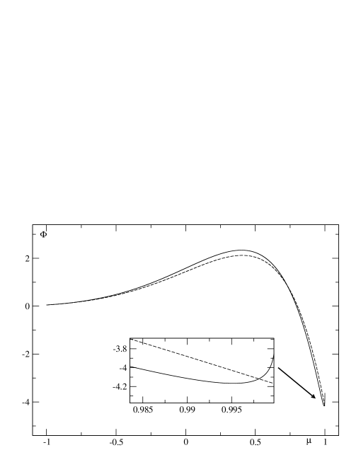
Figure 2: Unperturbed eigenfunction $\Phi\left(\mu\right)\equiv\Psi_{\lambda_{1}}^{\left(0\right)}$ (numerical solution of eq.[17], dashed line). Perturbed solution (eqs.[19] and [23], solid line). The insert shows the solution behavior at the end point, including the logarithmic term of the outer solution.

To find $\lambda^{\left(0\right)}$ we require the solution to be regular at the both singular points $\mu=\pm 1$. The solution of this problem can be found by a number of numerical methods, for example, by decomposing $\Psi_{\lambda}^{\left(0\right)}$ in a series of Legendre polynomials (e.g., Kirk & Schneider, 1987, and references therein). Since we have set $u=0$ (as opposed to the cited paper where $u\simeq 1)$, as few as the first six polynomials would suffice, with a cubic equation for $\lambda$. However, eq.(17) contains no parameters (except $\lambda$, of course) so that the most practical approach is to find the required single eigenvalue $\lambda_{1}$ and the corresponding eigenfunction by a direct numerical integration of the above equation. The result is shown in Fig.2 and $\lambda_{1}\approx 14.54$. Since $\lambda_{2}\simeq 2\lambda_{1}$, the WKB approximation can be applied for all $\lambda\geq\lambda_{2}$ points of the spectrum. However, the first eigenfunction and the eigenvalue $\lambda_{1}$ is sufficient for our purposes.

Since $D\equiv 1$ in the outer region, the perturbation can be associated only with the perturbation of $\lambda$. Therefore, we expand $\lambda$ and $\Psi_{\lambda}$ as

$$\lambda=\lambda^{\left(0\right)}+\delta\lambda+\dots$$ (18)

$$\Psi_{\lambda}=\Psi_{\lambda}^{\left(0\right)}+\delta\lambda\Psi_{\lambda}^{\left(1\right)}+\dots$$ (19)

Here $\lambda$ can be an arbitrary point of the spectrum $\lambda=\lambda_{i}>0$, but we are primarily interested in the case $\lambda=\lambda_{1}$. The equation for $\Psi_{\lambda}^{\left(1\right)}$ takes the following form

$$\frac{d}{d\mu}\left(1-\mu^{2}\right)\frac{d\Psi_{\lambda}^{\left(1\right)}}{d\mu}+\lambda^{\left(0\right)}\mu\Psi_{\lambda}^{\left(1\right)}=-\mu\Psi_{\lambda}^{\left(0\right)}$$ (20)

Since the r.h.s. of this equation is not orthogonal to the solution of its homogeneous part (eq.[17]), the operator on the l.h.s. of eq.(20) is not identical to that in eq.(17). Namely, the regularity condition at $\left|\mu\right|=1$ no longer applies. Instead, a singular, linearly independent counterpart of the solution of eq.(17) should be included (which is appropriate for the outer solution, but which is not for the inner solution that will be considered in the next subsection). Note that being interested in the behavior of the overall solution near $\mu=1$, we can still require the solution being regular at $\mu=-1$, since the unperturbed eigenfunction is small there ( e.g., Fig. 2) and the perturbation at $\mu\simeq-1$ does not significantly influence the overall behavior of the solution. With this in mind, we can write the solution of the last equation as follows

$$\Psi_{\lambda}^{\left(1\right)}=-\Phi\intop_{-1}^{\mu}\frac{U\left(\mu^{\prime}\right)d\mu^{\prime}}{\Phi^{2}\left(\mu^{\prime}\right)\left(1-\mu^{\prime 2}\right)}$$ (21)

where we have denoted $\Phi\left(\mu\right)\equiv\Psi_{\lambda}^{\left(0\right)}\left(\mu\right)$, and

$$U\left(\mu\right)\equiv\intop_{-1}^{\mu}\mu^{\prime}\Phi^{2}\left(\mu^{\prime}\right)d\mu^{\prime},$$ (22)

for short. Two further remarks are in order here. First, the above solution diverges logarithmically when $\mu\to 1$. But, it is not applicable within $1-\mu\mathrel{\mathchoice{\vbox{\offinterlineskip\halign{\hfil\(\displaystyle#\)\hfil\cr$\displaystyle<$\cr$\displaystyle\sim$\cr}}}{\vbox{\offinterlineskip\halign{\hfil\(\textstyle#\)\hfil\cr$\textstyle<$\cr$\textstyle\sim$\cr}}}{\vbox{\offinterlineskip\halign{\hfil\(\scriptstyle#\)\hfil\cr$\scriptstyle<$\cr$\scriptstyle\sim$\cr}}}{\vbox{\offinterlineskip\halign{\hfil\(\scriptscriptstyle#\)\hfil\cr$\scriptscriptstyle<$\cr$\scriptscriptstyle\sim$\cr}}}}\epsilon$, where an inner expansion should be obtained and matched to the solution, given by the outer expansion, eqs.(19) and (21). Second, the integral in eq.(21) is improper because $\Phi\left(\mu\right)$ has zeroes, in particular the one at $\mu=\mu_{1}\simeq 0.8$ for $\lambda=\lambda_{1}$. The integral should be understood in terms of a principle value and the solution behaves at $\mu\approx\mu_{1}$ as $\Psi_{\lambda_{1}}^{\left(1\right)}\propto\left(\mu-\mu_{1}\right){\rm ln}\left|\mu-\mu_{1}\right|$. Before we turn to the inner part of the solution, for the purpose of matching, it is convenient to rewrite the outer solution, given by eq.(21), in the following form

$$\Psi_{\lambda}^{\left(1\right)} = \frac{U\left(1\right)}{2\Phi^{2}\left(1\right)}\Phi\left(\mu\right){\rm ln}\left(\frac{1-\mu}{2}\right)-\Phi\left(\mu\right)$$ (23)

$$\times \intop_{-1}^{\mu}\frac{d\mu^{\prime}}{1-\mu^{\prime}}\left[\frac{U\left(\mu^{\prime}\right)}{\left(1+\mu^{\prime}\right)\Phi^{2}\left(\mu^{\prime}\right)}-\frac{U\left(1\right)}{2\Phi^{2}\left(1\right)}\right]$$

Here the first term is singular at $\mu=1$ while the second term is regular there.

4.2 Angular distribution of the beam

Turning to the inner expansion of the solution of eq.(15), it is convenient to stretch the variable $\mu$ at $\mu=1$ as follows

$$w=\frac{1-\mu}{b}$$ (24)

Note that $b=\epsilon j_{1}^{2}/2$ is chosen in such a way that $D\left(w=1\right)\approx 1$ (see Sec.3). Therefore, we represent $D$ as

$$D\left(w\right)=\left\{\begin{array}[]{cc}a^{-1}F\left(w\right)+1,&w\leq 1\\ 1,&w>1\end{array}\right.$$ (25)

with

$$F\left(w\right)=\frac{\pi}{2}\frac{1}{j_{1}^{2}w}J_{1}^{2}\left(j_{1}\sqrt{w}\right),\ \ \ w\leq 1$$ (26)

and $F\equiv 0$ for $w>1$. Note that $a=\nu_{\vartheta}l/v\ll 1$, sec.3. Eq.(15) can be written as follows

$$\frac{d}{dw}\left[F\left(w\right)+a\right]\left(2-bw\right)w\frac{d\Psi_{\lambda}^{i}}{dw}+ba\lambda\left(1-bw\right)\Psi_{\lambda}^{i}=0$$ (27)

where the index $i$ stands for the ’inner’ solution. In contrast to the outer problem we must impose the regularity condition at $\mu=1$ ($w=0$). Since $F$ vanishes for $w>1$ the expansion of the solution of this equation should be sought for in a series of powers of $b$, not $ba$, as an inspection of the second term of the equation may suggest. The latter form of the expansion would be valid only for $w<1$, whereas we need to match the solution of eq.(27) with the outer solution at $w\mathrel{\mathchoice{\vbox{\offinterlineskip\halign{\hfil\(\displaystyle#\)\hfil\cr$\displaystyle>$\cr$\displaystyle\sim$\cr}}}{\vbox{\offinterlineskip\halign{\hfil\(\textstyle#\)\hfil\cr$\textstyle>$\cr$\textstyle\sim$\cr}}}{\vbox{\offinterlineskip\halign{\hfil\(\scriptstyle#\)\hfil\cr$\scriptstyle>$\cr$\scriptstyle\sim$\cr}}}{\vbox{\offinterlineskip\halign{\hfil\(\scriptscriptstyle#\)\hfil\cr$\scriptscriptstyle>$\cr$\scriptscriptstyle\sim$\cr}}}}1.$ While the regularity condition at $w=0$ fixes one of the two arbitrary constants of the solution, it is convenient to choose the second constant as the value of the solution at $w=0$, i.e., $\Psi_{\lambda}^{i}\left(0\right)$.

Working up to the second order in $b\ll 1$, and integrating eq.(27) by parts, we transform it into the following first order equation

$$\frac{d\Psi_{\lambda}^{i}}{dw}+\frac{\lambda b}{2}g^{\prime}\left[1-\frac{\lambda b}{2}\left(\frac{h}{w}-g\right)\right]\Psi_{\lambda}^{i}=0$$

with the following obvious solution

$$\Psi_{\lambda}^{i}\left(w\right)=\Psi_{\lambda}^{i}\left(0\right)\exp\left\{-\frac{\lambda b}{2}g\left(1+\frac{\lambda b}{4}g\right)+\frac{\lambda^{2}b^{2}}{4}\int_{0}^{w}g^{\prime}hdw/w\right\}$$ (28)

where we have used the notation

$$g\left(w\right)=a\intop_{0}^{w}\frac{dw^{\prime}}{F\left(w^{\prime}\right)+a}$$ (29)

and

$$h=\intop_{0}^{w}g\left(w^{\prime}\right)dw^{\prime}.$$

As it is seen from eq.(25), the function $g$ can be evaluated as follows

$$g = \left\{\begin{array}[]{cc}\frac{8}{\pi}aw,&w<1\\ g_{1}+w-1,&w\geq 1\end{array}\right.$$ (32)

where $g_{1}\simeq-\sqrt{2\pi a}/J_{0}\left(j_{1}\right)$. In order to match the inner solution given by eq.(28) with the outer solution obtained earlier (see eqs.[19,23]), we need to expand both solutions in power of $w$ or $1-\mu$ which are valid in an overlap region. This is obviously a region where $1-\mu\ll 1$ (to make a series expansion of the outer solution accurate) and $w>1$ (to make the inner solution simple, e.g., to use eq.[32] for $g$). As $w=\left(1-\mu\right)/b$ with $b\ll 1$, the overlap region exists. Let us write the outer solution given by eqs.(19,23) in terms of the inner variable

$$\Psi_{\lambda} = \Phi\left(1\right)-\Phi^{\prime}\left(1\right)bw+\frac{1}{2}\Phi^{\prime\prime}\left(1\right)b^{2}w^{2}$$ (33)

$$+ \frac{U\left(1\right)}{2\Phi\left(1\right)}\delta\lambda\left({\rm ln}w+{\rm ln}b\right)+\mathcal{O}\left(\delta\lambda+b^{3}\right)$$

where the primes denote the derivatives of $\Phi\left(\mu\right)$ at $\mu=1$. The first three terms of the last expression is nothing but the leading terms of the Frobenius expansion of the unperturbed regular part of the solution of eq.(17) at the singular end point $\mu=1$. The fourth term is a perturbative, singular part of expansion, which is entirely due to the fact that the spectral parameter $\lambda$ deviates from its eigenvalue, ie $\delta\lambda=\lambda-\lambda_{i}\neq 0$. The both expansions are written in terms of the inner variable $w>1$, and thus $D\left(\mu\right)=1$ in eq.(15).

The inner solution given by eq.(28) can be written for $w>1$ as follows

$$\Psi_{\lambda}^{i}=\Psi_{\lambda}^{i}\left(0\right)\left[1-\frac{1}{2}\lambda b\left(g_{1}+w-1\right)+\frac{1}{8}\lambda^{2}b^{2}\left(\frac{1}{2}w^{2}-2w+{\rm ln}w\right)\right]$$ (34)

Comparing the last two results, we deduce

$$\Psi_{\lambda}^{i}\left(0\right)\approx\frac{\Phi\left(1\right)}{1+\lambda b/2}$$ (35)

and

$$\delta\lambda=\frac{\lambda^{2}\Phi^{2}\left(1\right)}{4U\left(1\right)}b^{2}.$$ (36)

Using the matching procedure we determined the initially unknown arbitrary constant of the inner solution $\Psi_{\lambda}^{i}\left(0\right)$ and the perturbation of the eigenvalue $\lambda$ by matching the terms in both equations that are independent of $w$ and proportional to ${\rm ln}w$, respectively. The linear and quadratic terms in $w$ match automatically to the appropriate accuracy $\sim b^{2}$. This follows from the two further relations

$$\Phi^{\prime}\left(1\right)=\frac{\lambda}{2}\Phi\left(1\right),\;\;\;\;\Phi^{\prime\prime}\left(1\right)=\frac{\lambda}{4}\Phi^{\prime}\left(1\right),$$

which can be obtained from the Frobenius series of eq.(17) at the singular end point $\mu=1$ with $\Psi_{\lambda}^{(0)}\equiv\Phi$.

The following two observations are important for the goal of this paper. First, since $U\left(1\right)$ in eq.(22) is positive definite (which may be readily seen from the equation for $\Phi$, eq.[17], by multiplying it by $\Phi$ and integrating by parts), $\delta\lambda$ in eq.(36) is positive definite as well. Of course, this property of the spectrum can be seen directly from eq.(15) by virtue of the positive sign of the perturbation of the coefficient $D$. Second, the perturbed absolute value of the eigenfunction at $\mu=1$, given by eq.(35) is always less than the unperturbed one, i.e., $\left|\Psi_{\lambda}^{i}\left(0\right)\right|<\left|\Phi\left(1\right)\right|$. Below, we discuss the observational consequences of these results.

4.3 Observational Appearance of the Beam

After we have determined the angular distribution of the beam, the question is whether it is consistent with at least the prominent MILAGRO hot spot A (Abdo et al., 2008). There are two observationally testable properties of the solution. The first property is that the sign of the perturbative correction to the distribution function is opposite, according to eqs.(34,35), to the sign of $\Phi\left(1\right)$. Of course, the latter can be changed arbitrarily but then the main expansion coefficient, eqs.(14,16) will change its sign as well. Let us fix $\Phi\left(1\right)\equiv\Psi_{\lambda_{1}}^{\left(0\right)}\left(1\right)<0$, as shown in Fig.2. Then, the perturbative correction will produce a logarithmic peak at $\mu=1$ if $C_{\lambda_{1}}>0$ and a negative logarithmic hole in the opposite case. As it may be seen from eq.(16) and Fig.2, the requirement $C_{\lambda_{1}}>0$ constrains the initial distribution $f_{0}\left(\mu\right)$ as follows. While being enhanced in the region $\mu>0$ (particles propagate predominantly away from the source towards the Earth), $f_{0}\left(\mu\right)$ should not be concentrated too close to $\mu\approx 1$. One simple conclusion from this observation is that if an accelerator at $z=0$ produces a beam of leaking particles, this beam should not be collimated tightly at $\mu=1$, or even overpopulate the region $\mu_{1}<\mu<1$, where $\Phi\left(\mu_{1}\right)=0$ with $\mu_{1}\simeq 0.8$.

The second property of the solution is that the bump on the particle angular distribution is located at the local minimum of the unperturbed eigenfunction. This is formally not consistent with the MILAGRO results. On the contrary, the latter indicate that the bump is in the region of monotonic change of the distribution function. However, the particle distribution obtained above is coming only from the flux tube that connects the Earth with the source of the beam. Therefore, to obtain the total distribution, the CR background anisotropic component should be added. The latter, being independent of the beam source, is most likely to change monotonically in any randomly selected area, such as the MILAGRO hot spot A, so there is no apparent contradiction in this regard.

In Sec. 4.2 the two major beam parameters were calculated in terms of the small parameter of the theory,

$$\epsilon=\frac{r_{g}\left(p\right)}{l}$$

where $r_{g}$ is the particle gyro-radius and $l$ is maximum wave length beyond which particles interact with waves adiabatically. The first parameter of the beam is its angular width (in terms of $\mu=\cos\vartheta$)

$$b=\frac{j_{1}^{2}}{2}\epsilon\approx 7.3\epsilon$$ (37)

and the second is its strength, which can be conveniently expressed as the ratio of the beam excess to the amplitude of the first eigenfunction, eq.(35)

$$\frac{\delta\Phi\left(1\right)}{\Phi\left(1\right)}\approx\frac{1}{2}\lambda_{1}b\approx 53.4\epsilon$$ (38)

Since $\epsilon\propto p$, the spectrum of the beam should be one power harder than the CR large scale anisotropic component inside the flux tube. This is consistent with the Milagro beam spectrum, provided that $\Phi$ scales with momentum similarly to the galactic CR background.

According to the MILAGRO Region A observations, the beam width is about $\Delta\vartheta\sim 10^{\circ}$, where $\Delta\vartheta\approx\cos^{-1}\left(1-b\right)\approx\sqrt{2b}=j_{1}\sqrt{\epsilon}$ so that we obtain for $\epsilon$ the following constraint from the observed MILAGRO Spot A

$$\epsilon\approx\left(\frac{\Delta\vartheta}{j_{1}}\right)^{2}\approx 2.1\cdot 10^{-3}.$$

This estimate yields the strength of the beam given by eq.(38) at the level of $\approx 0.1$ which is also consistent with the MILAGRO fractional excess of the beams A and B measured with respect to the large scale anisotropy.

In this section we made a preliminary consistency check of the beam, as it forms while the large scale anisotropic CR distribution propagates from its source to the Earth. In the next section we verify conditions under which the beam can really reach the Earth without self-destruction, as it is well known that beams in plasmas readily go unstable.

4.4 Beam Sustainability

Now that we have calculated the pitch-angle distribution of a narrow CR beam formed from a wide angle anisotropic CR flux by its interaction with the background ISM turbulence, we need to check whether the beam will survive the pitch-angle scattering by self-generated waves. The threat is the cyclotron instability of the beam but the hope (as already mentioned by Drury & Aharonian (2008) in regard with the magnetic nozzle) is the isotropic part of the CR background distribution which should stabilize the beam. The dispersion relation is a standard one, which can be written as follows (see e.g., Achterberg, 1983)

$$1-\frac{\omega^{2}}{k^{2}V_{A}^{2}}+\frac{4\pi^{2}e^{2}}{k}\int\frac{p_{\perp}^{2}dp_{\perp}dp_{\parallel}}{p^{2}\left(kv_{\parallel}\pm\omega_{c}-\omega\right)}$$

$$\times\left[p_{\perp}\frac{\partial F}{\partial p_{\parallel}}-\left(p_{\parallel}-\frac{\omega p}{kc}\right)\frac{\partial F}{\partial p_{\perp}}\right]=0$$ (39)

where $\pm$ signs correspond to the left/right polarized Alfven waves propagating along the field line at the Alfven speed $V_{A}$ ($k\approx k_{\parallel},\,$$\omega\approx\pm kV_{A}$). The distribution function $F\left(p_{\parallel},p_{\perp}\right)$ refers to the sum of the isotropic CR background distribution $F_{C}$, the beam distribution $F_{B}$, and a large scale anisotropic part $F_{1}\left(p_{\parallel},p_{\perp}\right)$. The latter, in turn, consists of both the unperturbed solution $\Phi\left(\mu,p\right)$, obtained in Sec.4.1 and the background large scale anisotropic component, most likely not related to the source of the beam. Thus, the total distribution function can be represented as $F=F_{C}\left(p\right)+F_{B}\left(p_{\parallel},p_{\perp}\right)+F_{1}\left(p_{\parallel},p_{\perp}\right)$. Since the beam is concentrated at small pitch angles, i.e., $0<p_{\perp}\ll p_{\parallel}$, we assume its contribution to be larger than that of $F_{1}$. Clearly, both $F_{C}$ and $F_{B}$ are small compared to the background plasma density which yields the second term in eq.(39).

To simplify the calculations, it is convenient to introduce the new variable $\rho$, instead of $p_{\perp}$

$$\rho=p-\delta p_{\parallel}\equiv\sqrt{p_{\parallel}^{2}+p_{\perp}^{2}}-\delta p_{\parallel}$$

here $\delta=\pm V_{A}/c$, where $\pm$ relates to the forward and backward propagating waves ($\omega=\pm kV_{A}$), respectively. Note that the lines of constant $\rho$ coincide with the lines of quasilinear diffusion of the distribution function $F$ and with the direction of differentiation in the brackets in eq.(39). On writing, $\omega=\pm kV_{A}+\gamma$, ($\gamma\ll kV_{A}$) and neglecting a small term $\delta\ll 1$ in the resonance denominator of eq.(39), we obtain for the wave growth-rate the following relation

$$\gamma=\frac{2\pi^{3}e^{2}}{\left|k\right|}\delta\int\frac{p_{\perp}^{3}}{p}\delta\left(p_{\parallel}\pm\frac{eB_{0}}{kc}\right)\left.\frac{\partial F}{\partial p_{\parallel}}\right|_{\rho}dp_{\perp}dp_{\parallel}.$$

Since $F_{C}=F_{C}\left(p\right)$ and $\left.\partial F_{C}/\partial p_{\parallel}\right|_{\rho}\approx\delta\partial F_{C}/\partial p$, the contribution of $F_{C}$ into the growth-rate is stabilizing ($\partial F_{C}/\partial p<0$) for both signs of $\delta$ and both wave polarizations. The contribution of the beam is destabilizing, also for both polarizations, as long as the real part of the frequency is taken as $\omega\approx+kV_{A}$, i.e., $\delta>0$. If the beam density were above the instability threshold, it would rapidly spread in pitch angle on the self-generated waves along the lines $\rho=const$. Therefore, the beam momentum distribution can be obtained from the instability threshold condition, i.e., from an assumption that the imaginary contributions from the beam and from the background CRs cancel. Thus, splitting the total distribution as $F=F_{C}\left(p\right)+F_{B}\left(p_{\parallel},p_{\perp}\right)$ and integrating the term with $F_{B}$ by parts in $p_{\perp}$, we obtain for the growth rate ($0<\delta\ll 1$)

$$\gamma = \frac{2\pi^{3}e^{2}}{\left|k\right|}\delta\intop_{0}^{\infty}\frac{p_{\perp}^{3}}{p^{2}}dp_{\perp}dp_{\parallel}\delta\left(p_{\parallel}-\frac{eB_{0}}{\left|k\right|c}\right)$$ (40)

$$\times \left(2\frac{p_{\parallel}^{2}}{p_{\perp}^{2}}F_{B}+\delta p\frac{\partial F_{c}}{\partial p}\right)$$

The beam contribution to the growth rate suggests to introduce a beam distribution integrated in $p_{\perp}$:

$$\mathcal{F}_{B}\left(p_{\parallel}\right)\equiv\frac{1}{p_{\parallel}^{2}}\int p_{\perp}F_{B}\left(p_{\perp},p_{\parallel}\right)dp_{\perp}$$ (41)

Note that for the beam particles $p_{\parallel}\approx p$. Assuming a power-law momentum scaling for $F_{C}\left(p\right)\propto p^{-q_{c}}$ (with $q_{c}=4.6-4.7$, appropriate for the background CR momentum distribution) from eq.(40) we can obtain an expression for the instability threshold distribution $\mathcal{F}_{th}\left(p_{\parallel}\right)$. As we noted, this is the beam distribution that cancels $\gamma$ in eq.(40):

$$\mathcal{F}_{th}\left(p_{\parallel}\right)\equiv\frac{\delta}{q_{c}-2}F_{C}\left(p_{\parallel}\right)$$ (42)

so that if $\mathcal{F}_{B}\left(p_{\parallel}\right)\leq\mathcal{F}_{th}\left(p_{\parallel}\right)$, the beam can sustain its angular distribution. Otherwise, it will be spread in pitch angle to satisfy the last inequality. Assuming, however that this inequality holds, we calculate $\mathcal{F}_{B}$ using our results from the previous section. First, unlike the threshold function $\mathcal{F}_{th}\left(p_{\parallel}\right)$ which is determined by the isotropic CR background, the momentum dependence of $\mathcal{F}_{B}\left(p_{\parallel}\right)$ is prescribed by the wide angle anisotropic component, denoted earlier as $\Phi\left(\mu\right)$, eqs.(33-35) and (38). The particle momentum entered this function as a parameter (which we omitted, for short) since we were considering only the pitch-angle scattering under the conserved momentum. Using the expressions for the width of the beam and for its amplitude relative to $\Phi\left(\mu,p\right)$ given by eqs.(37) and (38), respectively, we can represent $\mathcal{F}_{B}\left(p_{\parallel}\right)$ as follows

$$\mathcal{F}_{B}\left(p_{\parallel}\right)=\frac{\lambda_{1}b^{2}}{2}F_{0}\left(p_{\parallel}\right)=\frac{1}{8}\lambda_{1}j_{1}^{4}\epsilon^{2}F_{0}\left(p_{\parallel}\right)$$ (43)

where we have denoted $F_{0}\left(p\right)\equiv\Phi\left(\mu=1,p\right)$. Then, our constraint $\mathcal{F}_{B}\left(p_{\parallel}\right)\leq\mathcal{F}_{th}\left(p_{\parallel}\right)$ can be represented in the following way

$$F_{0}\left(p\right)\leq A\frac{V_{A}}{c}\frac{l^{2}}{r_{g}^{2}\left(p\right)}F_{C}\left(p\right)$$ (44)

where $r_{g}=pc/eB_{0}$ is the particle gyro-radius. We denoted by $A$ the following numerical factor

$$A=\frac{8}{\lambda_{1}j_{1}^{4}\left(q_{c}-2\right)}\approx 10^{-3}$$

Due to the factor $r_{g}^{-2}$ in the relation given by eq.(44), the function $F_{0}\left(p\right)$ is constrained at high momenta. Assuming that $F_{0}$ is not much steeper than the background distribution $F_{C}$, we infer from eq.(44) that there exists maximum momentum $p_{Bmax}$, beyond which the beam would spread in pitch-angle and dissolve in the CR background. In fact we can extract more information from the last constraint. To conform with the Milagro results, we assume $F_{0}\sim\tilde{F}_{C}$, where $\tilde{F}_{C}$ is the anisotropic part of the CR background distribution. It is known to be about $\alpha\sim 10^{-3}$ of the isotropic part $F_{C}$, so we can estimate $F_{0}\sim\alpha F_{C}$. The last estimate along with eq.(44) brings us to the maximum beam energy

$$\frac{p_{Bmax}}{mc}\simeq\frac{1}{K}\sqrt{\frac{V_{A}}{c}\frac{A}{\alpha}}$$ (45)

where we have introduced the following parameter which is the major small parameter of the theory

$$K\equiv\frac{c}{l\omega_{c}}=\epsilon\frac{mc}{p}.$$ (46)

Here $\omega_{c}$ is the proton cyclotron (non-relativistic) frequency and $l$ is the maximum turbulence scale beyond which the particles response becomes adiabatic. Based on the two independent MILAGRO measurements of the width and the fractional excess of the Beam A, we inferred earlier the parameter $\epsilon\sim 10^{-3}$. Assuming that this value of $\epsilon$ relates to the $1$TeV median energy of the MILAGRO collaboration angular analysis, we obtain for $K$ the value $K\sim 10^{-6}$. Taking $V_{A}/c\sim 10^{-4}$ and $\alpha\sim A\sim 10^{-3}$, we obtain $p_{Bmax}\sim 10$ TeV. This is encouragingly close to the MILAGRO estimates of the beam cut-off energy. We will consider approaches to the independent determination of the theory small parameter $K$ and the beam maximum momentum in the next section. Of course, depending on which of the Milagro beam measurements (the width, excess or cut-off momentum) is the most reliable, this quantity may be used to determine $K$ or $l$.

To conclude this section, we estimate the possible losses of the beam due to the energy dependent curvature and gradient drifts. Assuming $\nabla\times\mathbf{B}=0$ and a small propagation angle to the magnetic field (curvature drift dominates), the particle drift velocity can be written as

$$\mathbf{V}_{cd}=\frac{p}{mc}\frac{c^{2}}{\omega_{c}B^{2}}\mathbf{B}\times\nabla B$$ (47)

We can estimate particle displacement across the field line upon traveling a distance of one correlation length $l_{B}$ as $\Delta r\sim r_{g}\left(p\right)l_{B}/R$, where $R$ is the typical field curvature. The total displacement from the field line is thus $r\sim r_{g}\sqrt{L_{S}l_{B}}/R\sim r_{g}\sqrt{L_{S}/l}$ where $L_{S}$ is the distance from the source to the observer. The displacement $r$ may be not much larger than the SNR radius, for example, so there should be no significant loss of particle flux due to the drift related spreading.

5 Distance to the source, beam energy window and the maximum scale $l$

Assuming only one free parameter $K=c/l\omega_{c}$ with $l$ being an (unknown a priori) scale of turbulence beyond which particles are not scattered in pitch angle, we have advanced our theoretical construction to the point where it successfully matches the three major MILAGRO observables. These are the angular width of the beam, its excess and its maximum momentum $p_{Bmax}$. Each of those three quantities consistently points at the same value of $K\sim 10^{-6}$ or $l\sim 1pc/B_{\mu G}$. In this section we relate $K$ to the further two independent quantities. One of these quantities is the maximum momentum $p_{max}$ of the CRs accelerated in the SNR which may be responsible for the MILAGRO beam. The other quantity is the distance to this remnant, $L_{s}$, or to any other source of energetic particles from which the beam originates. Starting from the source, we represent the decay of the large scale anisotropic part of the distribution function as follows (see eqs.[11,12] and [14])

$$F_{S}\left(z,p\right)\sim F_{S}\left(0,p\right)\exp\left[-\mathcal{L}^{-1}\frac{z}{l}\right]$$ (48)

where $\mathcal{L}^{-1}\left(\epsilon\right)$ is the inverse dimensionless particle scattering length

$$\mathcal{L}^{-1}\left(\epsilon\right)=\frac{\lambda_{1}}{6}\left(\delta{\rm ln}\frac{1}{\epsilon}+\epsilon^{3/2}\right)$$

and $F_{S}\left(0,p\right)$ is the anisotropic part of the distribution at the source. As we argued earlier, for the beam to appear at the Earth ($z=L_{S}$) as observed, $F_{S}\left(L_{S},p\right)$ should be of the order of the anisotropic part of the local background CRs. Moreover, $\mathcal{L}^{-1}\left(\epsilon\right)$ has a minimum ($\approx 1.7\cdot 10^{-3}$) at $\epsilon=\left(2\delta/3\right)^{2/3}\simeq 1.6\cdot 10^{-3}$ for $\delta\equiv V_{A}/c=10^{-4}$. This value of $\epsilon$ is remarkably close to that inferred earlier from the Milagro measurements of the beam width and its fractional excess ($\epsilon\simeq 2\cdot 10^{-3}$). Since $\epsilon\propto p$, the anisotropic part $F_{S}\left(z,p\right)$ decays rapidly with $p$. Therefore, for the beam to be observable at $10$ TeV, the distance $L_{s}$ should not significantly exceed the quantity

$$L_{Smax}\approx\frac{6l}{\lambda_{1}\epsilon^{3/2}\left(p_{Bmax}\right)}Ln$$ (49)

with

$$Ln={\rm ln}\frac{F_{s}\left(0,p\right)}{F_{s}\left(L_{Smax},p\right)}$$

which can be recast as

$$L_{Smax}\simeq 0.4\frac{c}{\omega_{c}}\left(\frac{mc}{p_{Bmax}}\right)^{3/2}K^{-5/2}Ln$$

or, assuming $K=10^{-6}$, as inferred from the Milagro Spot A parameters, and $B=3\mu G$, we obtain

$$L_{Smax}\simeq 130\cdot Ln\cdot\left(\frac{10TeV}{E_{Bmax}}\right)^{3/2}pc.$$ (50)

Given that $Ln$ may be a factor of a few, the last estimate constrains the distance to any SNR, held responsible for the Milagro beam, to a few hundreds of parsecs. In fact there is also the lower bound to $L_{S}$ which, being formally a technical one, may still be meaningful. Indeed, in our calculations of the beam profile, we neglected the contributions of the eigenfunctions corresponding to the eigenvalues $\lambda_{n}$ with $n\geq 2$. Since $\lambda_{2}\simeq 2\lambda_{1}$, the neglected terms in the spectral expansion of the distribution function would not contribute near $p\sim p_{Bmax}$, but they could become essential at lower momenta where $\mathcal{L}^{-1}$ has a minimum as a function of $p$. That is why we required in Sec.4 $\mathcal{L}^{-1}\frac{z}{l}\mathrel{\mathchoice{\vbox{\offinterlineskip\halign{\hfil\(\displaystyle#\)\hfil\cr$\displaystyle>$\cr$\displaystyle\sim$\cr}}}{\vbox{\offinterlineskip\halign{\hfil\(\textstyle#\)\hfil\cr$\textstyle>$\cr$\textstyle\sim$\cr}}}{\vbox{\offinterlineskip\halign{\hfil\(\scriptstyle#\)\hfil\cr$\scriptstyle>$\cr$\scriptstyle\sim$\cr}}}{\vbox{\offinterlineskip\halign{\hfil\(\scriptscriptstyle#\)\hfil\cr$\scriptscriptstyle>$\cr$\scriptscriptstyle\sim$\cr}}}}1$. It does not mean, however, that the beam would not form at these momenta but its shape may change. Unfortunately, the available Milagro data are not sufficient to distinguish between the cases of single and multiple beam eigenfunctions. Nevertheless the apparent absence of a mesoscale anisotropy (i.e., scales between the narrow beam and the first angular harmonics) hints at a relative unimportance of the higher eigenfunction in the spectral expansion. If this is the case, then the upper bound on $L_{S}$ given by eq.(50) should be rather close to the lower bound as well.

Let us turn to the question of determining the scale $l$. The simplest possibility is to associate $l$ with the outer scale of the ISM turbulence. Its typical estimates extend from 1pc (spiral arms) up to 100 pc for the inter-arm space Haverkorn et al., 2008. However, a 100pc scale can hardly be relevant to our analysis already for that simple reason that the Larmor radii of particles of interest are five order of magnitude smaller. Clearly, such long scales should be attributed to the ambient field rather than to the particle scattering field component. On the other hand, as the turbulent energy injected at such long scales cascades to much shorter scales where the wave can interact with $1-10$ TeV particles, the spectral energy density is already too low to provide efficient scattering. Clearly, a realistic estimate of outer scale of turbulence $l$, relevant for the wave-particle interaction, should be somewhere between these extremes. If particles are propagating from an accelerator, there must be energy injection into the GS cascade at a scale, associated with this accelerator. Obviously, $l$ cannot exceed the accelerator (shock) radius. It is interesting to note that the recent optical observations of the SNR 1006 indicate that ripples on the shock surface have a scale ~1pc (Raymond et al., 2007), which is the preferred scale to match the Milagro data. From the theoretical standpoint, we need to make an assumption about the accelerator. There are a few possibilities, such as a nearby SNR or a massive blue star surrounded by a wind bubble with the termination shock. Each of these, being magnetically connected with the Earth may accelerate particles and load the connecting flux rope with both the accelerated particles and Alfvenic turbulence. In order to avoid further uncertainties associated with the accelerator, we assume that the turbulence is driven primarily by escaping particles. This is almost certainly the case, once particles escape at the rate sufficient to be detected at the Earth. The turbulence, however may significantly decay along the flux rope due to the relaxation of initially strongly unstable (anisotropic) particle distribution and due to lateral losses of particles and waves. Note that if these are significant, one should replace $zD\left(\mu\right)\to\int Ddz$ in our treatment of particle propagation in Sec.4.

The mechanisms of particle escape from a SNR shock, for example, are many (Drury et al., 1996; Malkov et al., 2002; Malkov & Diamond, 2006; Caprioli et al., 2009; Reville et al., 2009). In almost all cases the escaping particles are close to the maximum energy achievable in the accelerator and have an anisotropic momentum distribution. Therefore they should drive Alfven waves at a scale $l\sim r_{g}\left(p_{max}\right)$. Since $r_{g}\left(p\right)\simeq 10^{-6}B_{\mu G}^{-1}\left(p/mc\right)$pc, to recover the scale $l\sim 1$ pc, inferred earlier from the beam parameters, it is necessary to assume $E_{max}\sim 3$ PeV (for $B_{\mu G}\sim 3$) or precisely the ’knee’ energy.

6 Summary and discussion

The principal results of this paper are as follows. Assuming only a large scale anisotropic distribution of CRs (generated, for example by a nearby accelerator, such as a SNR) and a Goldreich & Sridhar (1995) (GS) cascade of Alfvenic turbulence originating from some scale $l$, which is the longest scale relevant for the wave-particle interactions, we calculated the propagation of the CRs down their gradient along the interstellar magnetic field. It is found that the CR distribution develops a characteristic angular shape consisting of a large scale anisotropic part (first eigenfunction of the pitch-angle scattering operator) superposed by a beam, tightly focused in the momentum space in the local field direction. The large scale anisotropy carries the momentum dependence of the source, while both the beam angular width and its fractional excess (with respect to the large scale anisotropic component) grow with momentum (as $\sqrt{p}$ and $p$, respectively). Apart from the width and the fractional excess of the beam, the theory predicts its maximum momentum on the ground that beyond this momentum the beam destroys itself. All the three quantities are completely determined by the turbulence scale $l$. Even if $l$ is considered unknown, it can be inferred from any of the three independent MILAGRO measurements. These are the width, the fractional excess and the maximum energy of the beam, and all the three consistently imply the same scale $l\sim$1 pc. The calculated beam maximum momentum encouragingly agrees with that measured by MILAGRO (~10 TeV/c). The theoretical value for the angular width of the beam is found to be $\Delta\vartheta\simeq 4\sqrt{\epsilon}$, where $\epsilon=r_{g}\left(p\right)/l\ll 1$. The beam fractional excess related to the large scale anisotropic part of the CR distribution is $\simeq 50\epsilon$. Both quantities also match the Milagro results for $E\sim 1-2$ TeV. So the beam has a momentum scaling that is one power shallower than the CR carrier, it is drawn from. This finding will receive a due discussion.

Obviously, the determination of the absolute value of the beam excess would require the source intensity. For the lack of such information, an indirect inference was made in Sec.4.3 about the galactic CR (GCR) large scale anisotropy being of the same order as the large scale anisotropy responsible for the beam.

Below the rationale for this admission is given which we open with the following notations:

• $\tilde{F}_{GCR}$ and $\bar{F}_{GCR}$ are the large scale anisotropic and isotropic parts of the galactic (not assumed to be related to the source of the beam) distribution, respectively

• $\tilde{F}_{S}$ and $\bar{F}_{S}$ (i.e. $f_{\infty}$ in sec.4) are the similar quantities related to the source of the beam at the distance $L_{S}$

• $F_{B}$ is the beam distribution on the top of $\tilde{F}_{S}$

Unless the source of the beam is also responsible for the GCR, the quantities $\tilde{F}_{S}$ and $\tilde{F}_{GCR}$ are independent of each other and cannot be related since the source intensity, the distance to it, $L_{S}$ and the losses are unknown. Even if the beam and its carrier $\tilde{F}_{S}$ propagate without significant losses (or suffer similar losses), the current theory determines only a fractional excess $F_{B}/\tilde{F}_{S}\sim 50\epsilon$ (independent of $L_{S}$). For the same reasons we do not know what is the source contribution $\bar{F}_{S}$ into the total isotropic CR background $\bar{F}{}_{GCR}+\bar{F}_{S}$. However, since the beam A is not observed at the minimum of the (measured) total large scale $\tilde{F}_{S}+\tilde{F}_{GCR}$ as it would, were $\tilde{F}_{S}\gg\tilde{F}_{GCR}$ the case (see Fig.2), we infer $\tilde{F}_{GCR}\mathrel{\mathchoice{\vbox{\offinterlineskip\halign{\hfil\(\displaystyle#\)\hfil\cr$\displaystyle>$\cr$\displaystyle\sim$\cr}}}{\vbox{\offinterlineskip\halign{\hfil\(\textstyle#\)\hfil\cr$\textstyle>$\cr$\textstyle\sim$\cr}}}{\vbox{\offinterlineskip\halign{\hfil\(\scriptstyle#\)\hfil\cr$\scriptstyle>$\cr$\scriptstyle\sim$\cr}}}{\vbox{\offinterlineskip\halign{\hfil\(\scriptscriptstyle#\)\hfil\cr$\scriptscriptstyle>$\cr$\scriptscriptstyle\sim$\cr}}}}\tilde{F}_{S}$. Furthermore, since $F_{B}/\tilde{F}_{S}$ is calculated and $\tilde{F}_{S}+\tilde{F}_{GCR}$ is measured along with $F_{B}$, the both quantities $\tilde{F}_{S}$ and $\tilde{F}_{GCR}$ can also be determined.

We found that $F_{B}/\tilde{F}_{S}\sim 0.1$ for $l\sim 1$pc which was, in turn, deduced from two other independent measurements (beam width $\Delta\vartheta$ and its maximum energy $E_{Bmax}$). Since Milagro measurements indicate that $F_{B}/\left(\tilde{F}_{GCR}+\tilde{F}_{S}\right)\sim 0.1$, we conclude that $\tilde{F}_{S}\sim\tilde{F}_{GCR}$. A more specific relation between the two would not be meaningful since the measurements of $F_{B}\left(p\right)$ are rather limited. If particle losses from the flux tube are negligible, it follows that $\tilde{F}_{S}\left(L_{S}\right)\sim\tilde{F}_{S}\left(0\right)$ for $p\ll p_{Bmax}$ ($0$- being the source position).

These findings allow us to speculate about the possible source of the beam. First, if the source is an active accelerator that emits strongly anisotropic particle flux, the last relation implies that $\bar{F}_{S}\sim\tilde{F}_{S}$. Since by observations $\tilde{F}_{S}\ll\bar{F}_{GCR}$, such source cannot contribute significantly to the ’knee’ region at $\simeq 3$ PeV. In this case our inferences of $l$ from three independent measurements –all strikingly pointing at the $3$ PeV accelerator cut-off energy (with $l\sim r_{g}\left(E_{max}\right)$)– must be either a coincidence or a different mechanism couples the galactic ’knee’ particles with the scale of the turbulence that generates the beam. If it is not a coincidence and the source contributes significantly to the observed CR background, the escaping particle flux should be quasi-isotropic, $\tilde{F}_{S}\ll\bar{F}_{S}$ (to allow for $\bar{F}_{S}\sim\bar{F}_{GCR}$). In combination with the assumption that particles escape in the wide range 1TeV -3 PeV (to both form the beam and to inject MHD energy at the scale $l$), the source is unlikely to be an active accelerator, but rather a region of an enhanced CR density, with a steep cut-off at $\simeq 3$ PeV. The near isotropy at the source is not inconsistent with a currently working accelerator, but escape in such a broad energy range probably is. Indeed, at least the available (known to us) mechanisms, that offer a broad energy escape from a SNR along with the spectrum steepening (i.e., spectral break, starting 1-2 orders of magnitude below the cut-off, e.g., Malkov et al., 2005; Malkov & Diamond, 2006) seem to fall short to cover three orders of magnitude in energy. Moreover for the source to be a recent accelerator (such as a recent SNR, suggested by Erlykin & Wolfendale, 1997 with the spectrum $E^{-2}$) the mechanism should be found that makes the spectrum of the escaping particles at least $0.5$ steeper (and still steeper if the acceleration was strongly nonlinear). Combined with the nonlinear acceleration (which is required in Malkov & Diamond, 2006 model) this would make an acceptable spectrum but again, it is not clear how these particles can initiate the MHD cascade at such a long scale, to ensure the required value of $l$.

Our argument against the beam and the bulk CR $\tilde{F}_{GCR}$ coming from the same source is that the observed beam is not located at the minimum of the angular distribution of the first eigenfunction, so we need to allow for a second component. This is largely a technical limitation, stemming from 1-D transport model, in which $F_{B}$ and $\tilde{F}_{S}$ are coupled, as wells as from the single eigenfunction approximation. By removing this latter simplification alone (which is probably even necessary for an accurate description of $\tilde{F}_{S}$ at TeV- energies, Sec.5) the above constraint can be relaxed. Another possibility is a lateral diffusion and drifts of $\tilde{F}_{S}$-component from the flux tube.

An interesting obvious conjecture from the common origin of the beam and $\tilde{F}_{GCR}$ would be that the proton ’knee’ at $\simeq 3$ PeV is also of the same origin as the beam. However, the beam spectrum is calculated to be one power flatter than its carrier. According to Milagro the beam index is about $1.5$, so that the carrier should have an index $\simeq 2.5$ which is closer to the GCR than to a hypothetical ’recent SNR’. In particular, this would not support the single source hypothesis of the GCR ’knee’ Erlykin & Wolfendale (1997). Equally problematic would be an active accelerator scenario, unless the steepening mechanisms of the run-away CR mentioned above can be adopted after due modifications.

All told, the beam is likely to be at least partly drawn from the GCR (due to the relation between the indices $q_{B}\simeq q_{GCR}-1$) but the GS- turbulence that creates the beam must be driven by considerably more energetic, $\mathrel{\mathchoice{\vbox{\offinterlineskip\halign{\hfil\(\displaystyle#\)\hfil\cr$\displaystyle>$\cr$\displaystyle\sim$\cr}}}{\vbox{\offinterlineskip\halign{\hfil\(\textstyle#\)\hfil\cr$\textstyle>$\cr$\textstyle\sim$\cr}}}{\vbox{\offinterlineskip\halign{\hfil\(\scriptstyle#\)\hfil\cr$\scriptstyle>$\cr$\scriptstyle\sim$\cr}}}{\vbox{\offinterlineskip\halign{\hfil\(\scriptscriptstyle#\)\hfil\cr$\scriptscriptstyle>$\cr$\scriptscriptstyle\sim$\cr}}}}1$ PeV particles (due to the constraint, $l\simeq r_{g}$), unless the spiral-arm 1pc value Haverkorn et al. (2008) for $l$ is, indeed, acceptable. To explore the possibility of the GCR origin of the beam, an extension of the above model is necessary. At a minimum, the model should include the transport of energetic particles across the flux tube. On the other hand, the particle beaming processes should remain similar to that described in Sec.3. However, such consideration is out of the scope of this paper, particularly because the transport across the flux tube requires a separate study.

Yet another possibility is that the required GS cascade starts in the local interstellar cloud (LIC). It has a suitable size of $\sim 5$ pc (Redfield & Linsky, 2000) and there would be no problem with the spectrum slope since the beam would be drawn from the GCR with the ’right’ spectral index $q_{GCR}\simeq 2.7$. Whether the turbulence energy can be injected at the required scale remains to be studied. If it can, the above transport and beam focusing mechanism would be applicable since a parsec wave length and the GS cascade are the only requirements to draw the beam out of the background CR distribution.

To conclude, the model presented in this paper offers an explanation of the most pronounced Milagro beam A, while there are two more. One of them is the beam B, $\sim 50^{\circ}$ away from beam A and the second one is in the Cygnus loop area $\sim 100^{\circ}$ away. Any attempt to incorporate those two beams into our current model would be speculative. We merely note that the local ISM environment is complicated indeed thus offering many possibilities in explaining various CR anomalies ( e.g., Amenomori et al., 2007). Approaches to the explanation of all three beams based on such a complexity, could hardly pass the Occam’s razor test. In contrast, the model suggested in this paper is devoid of free parameters, if the knee energy at $\sim 3$PeV can be associated with the maximum CR energy of the source of the Beam A. Even though such an association is not proven, our propagation model predicts the following three beam characteristics: its width, fractional excess and maximum energy to be the functions of a single quantity, the longest wave-particle interaction scale $l$. They all give the correct MILAGRO values for $l\simeq 1$ pc, which is unlikely to be coincidental. However, the exact origin of this particular value remains unclear.

Appendix A Appendix

In this Appendix we provide a sketch of the derivation of the pitch-angle diffusion coefficient $D_{\mu\mu}$ for the anisotropic turbulence of Alfven waves suggested by Goldreich & Sridhar (1995). We follow a standard line of argument (e.g., Völk, 1973). However, we include the finite auto-correlation time as required by the GS spectrum. We start with the equation for the particle momentum $\mathbf{p}$:

$$\frac{d\mathbf{p}}{dt}=\Omega\mathbf{p}\times\mathbf{B}/B_{0}$$ (A1)

where $\Omega=eB_{0}/p$, $p\gg mc$ and $B_{0}$ is the magnitude of the unperturbed magnetic field $\mathbf{B}_{0}$, assumed to be in $z$-direction. We also decompose the total magnetic field $\mathbf{B}$ in the following standard way

$$\mathbf{B}=B_{0}\hat{z}+\sum_{\mathbf{k}}\mathbf{B_{\mathbf{k}}}e^{i\mathbf{kr}}$$ (A2)

where $\hat{z}$ is the unit vector along $z$-axis. Note that for the shear Alfven waves, $\mathbf{B_{k}}\perp\mathbf{k},\hat{\,z}$. As usual, we introduce a spherical coordinate system in the momentum space with the axis along the unperturbed magnetic field: $p_{\parallel}=p\mu=\mathbf{p}\cdot\hat{z}$, $p_{\perp}=p\sqrt{1-\mu^{2}}$, $p_{x}+ip_{y}=p_{\perp}\exp\left(i\phi\right)$. The corresponding notations in $\mathbf{k}$-space are $k_{\parallel}=\mathbf{k}\cdot\hat{z}$, $k_{x}+ik_{y}=k_{\perp}\exp\left(\alpha_{\mathbf{k}}\right),$ and similarly for $\mathbf{B_{k}}$: $B_{\mathbf{k},x}+iB_{\mathbf{k},y}=B_{\mathbf{k}}\exp\left(i\chi_{\mathbf{k}}\right)$, where $\chi_{\mathbf{k}}=\alpha_{\mathbf{k}}\pm\pi/2$, where the $\pm$ corresponds to the direction of the wave propagation, $\omega=\pm\left|k_{\parallel}\right|V_{A}$. With this notations, also using the relation

$$\mathbf{kr}=k_{\parallel}v_{\parallel}t-\xi\sin\left(\phi-\alpha_{\mathbf{k}}\right),$$

with $\xi=k_{\perp}v_{\perp}/\Omega$, from eq.(A1) we obtain

$$\frac{d\mu}{dt}=\pm\frac{\Omega}{B_{0}}\sqrt{1-\mu^{2}}\sum_{\mathbf{k},n}B_{\mathbf{k}}e^{ik_{\parallel}v_{\parallel}t+in\left(\Omega t-\phi_{0}+\alpha_{\mathbf{k}}\right)}\frac{n}{\xi}J_{n}\left(\xi\right)$$ (A3)

where $\phi_{0}$ comes from the unperturbed particle orbit $\phi=\phi_{0}-\Omega t$ and $J_{n}$ stands for the Bessel function. Denoting by $\Delta\mu$ the variation of $\mu$ in time $t$, for an ensemble averaged $\left\langle\Delta\mu^{2}\right\rangle$ we obtain

$$\left\langle\Delta\mu^{2}\right\rangle=\Omega^{2}\left(1-\mu^{2}\right)\sum_{\mathbf{k},n}\iintop_{0}^{t}dt^{\prime}dt^{\prime\prime}I\left(k_{\parallel},k_{\perp},t^{\prime}-t^{\prime\prime}\right)e^{\left(ik_{\parallel}v_{\parallel}+in\Omega\right)\left(t^{\prime}-t^{\prime\prime}\right)}\frac{n^{2}}{\xi^{2}}J_{n}^{2}\left(\xi\right)$$

where

$$I_{\mathbf{k}}\left(t^{\prime}-t^{\prime\prime}\right)=\left\langle B_{\mathbf{k}}\left(t^{\prime}\right)\bar{B}_{\mathbf{k}}\left(t^{\prime\prime}\right)\right\rangle/B_{0}^{2}$$

is assumed to be axially symmetric in $\mathbf{k}-$space. Extracting the secular term from the last equation, we obtain eq.(1). Note that it can be further simplified by performing the summation in $n$

$$D_{\mu\mu}=-\left(1-\mu^{2}\right)\sum_{\mathbf{k}}\frac{1}{\xi^{2}}\intop_{0}^{\infty}I\left(k_{\parallel},k_{\perp},\tau\right)e^{ik_{\parallel}v_{\parallel}\tau}d\tau\frac{\partial^{2}}{\partial\tau^{2}}J_{0}\left(2\xi\sin\frac{\Omega\tau}{2}\right).$$

References

- Abdo et al. (2008) Abdo, A. A., Allen, B., Aune, T., Berley, D., Blaufuss, E., Casanova, S., Chen, C., Dingus, B. L., Ellsworth, R. W., Fleysher, L., Fleysher, R., Gonzalez, M. M., Goodman, J. A., Hoffman, C. M., Hüntemeyer, P. H., Kolterman, B. E., Lansdell, C. P., Linnemann, J. T., McEnery, J. E., Mincer, A. I., Nemethy, P., Noyes, D., Pretz, J., Ryan, J. M., Parkinson, P. M. S., Shoup, A., Sinnis, G., Smith, A. J., Sullivan, G. W., Vasileiou, V., Walker, G. P., Williams, D. A., & Yodh, G. B. 2008, Physical Review Letters, 101, 221101
- Achterberg (1983) Achterberg, A. 1983, A&A, 119, 274
- Amenomori et al. (2007) Amenomori, M., Ayabe, S., Bi, X. J., Chen, D., Cui, S. W., Danzengluobu, Ding, L. K., Ding, X. H., Feng, C. F., Feng, Z., Feng, Z. Y., Gao, X. Y., Geng, Q. X., Guo, H. W., He, H. H., He, M., Hibino, K., Hotta, N., Hu, H., Hu, H. B., Huang, J., Huang, Q., Jia, H. Y., Kajino, F., Kasahara, K., Katayose, Y., Kato, C., Kawata, K., Labaciren, Le, G. M., Li, A. F., Li, J. Y., Lou, Y., Lu, H., Lu, S. L., Meng, X. R., Mizutani, K., Mu, J., Munakata, K., Nagai, A., Nanjo, H., Nishizawa, M., Ohnishi, M., Ohta, I., Onuma, H., Ouchi, T., Ozawa, S., Ren, J. R., Saito, T., Saito, T. Y., Sakata, M., Sako, T. K., Sasaki, T., Shibata, M., Shiomi, A., Shirai, T., Sugimoto, H., Takita, M., Tan, Y. H., Tateyama, N., Torii, S., Tsuchiya, H., Udo, S., Wang, B., Wang, H., Wang, X., Wang, Y. G., Wu, H. R., Xue, L., Yamamoto, Y., Yan, C. T., Yang, X. C., Yasue, S., Ye, Z. H., Yu, G. C., Yuan, A. F., Yuda, T., Zhang, H. M., Zhang, J. L., Zhang, N. J., Zhang, X. Y., Zhang, Y., Zhang, Y., Zhaxisangzhu, & Zhou, X. X. 2007, 932, 283
- Bell (2004) Bell, A. R. 2004, MNRAS, 353, 550
- Beresnyak & Lazarian (2009) Beresnyak, A., & Lazarian, A. 2009, ApJ, 702, 1190
- Beresnyak et al. (2010) Beresnyak, A., Yan, H., & Lazarian, A. 2010, ArXiv e-prints
- Caprioli et al. (2009) Caprioli, D., Blasi, P., & Amato, E. 2009, MNRAS, 396, 2065
- Chandran (2000) Chandran, B. D. G. 2000, Physical Review Letters, 85, 4656
- Cho & Vishniac (2000) Cho, J., & Vishniac, E. T. 2000, ApJ, 539, 273
- Drury & Aharonian (2008) Drury, L. O. C., & Aharonian, F. A. 2008, Astroparticle Physics, 29, 420
- Drury et al. (1996) Drury, L. O. C., Duffy, P., & Kirk, J. G. 1996, A&A, 309, 1002
- Drury & Falle (1986) Drury, L. O. C., & Falle, S. A. E. G. 1986, MNRAS, 223, 353
- Ellison et al. (1996) Ellison, D. C., Baring, M. G., & Jones, F. C. 1996, ApJ, 473, 1029
- Erlykin & Wolfendale (1997) Erlykin, A. D., & Wolfendale, A. W. 1997, Journal of Physics G Nuclear Physics, 23, 979
- Goldreich & Sridhar (1995) Goldreich, P., & Sridhar, S. 1995, ApJ, 438, 763
- Goldreich & Sridhar (1997) —. 1997, ApJ, 485, 680
- Gurevich (1961) Gurevich, A. V. 1961, Soviet Journal of Experimental and Theoretical Physics, 12, 904
- Haverkorn et al. (2008) Haverkorn, M., Brown, J. C., Gaensler, B. M., & McClure-Griffiths, N. M. 2008, ApJ, 680, 362
- Jokipii (1966) Jokipii, J. R. 1966, ApJ, 146, 480
- Kang et al. (1992) Kang, H., Jones, T. W., & Ryu, D. 1992, ApJ, 385, 193
- Kennel & Engelmann (1966) Kennel, C. F., & Engelmann, F. 1966, Physics of Fluids, 9, 2377
- Kirk & Duffy (1999) Kirk, J. G., & Duffy, P. 1999, Journal of Physics G Nuclear Physics, 25, 163
- Kirk & Schneider (1987) Kirk, J. G., & Schneider, P. 1987, ApJ, 315, 425
- Kruskal & Bernstein (1964) Kruskal, M. D., & Bernstein, I. B. 1964, Physics of Fluids, 7, 407
- Malkov & Diamond (2006) Malkov, M. A., & Diamond, P. H. 2006, ApJ, 642, 244
- Malkov et al. (2002) Malkov, M. A., Diamond, P. H., & Jones, T. W. 2002, ApJ, 571, 856
- Malkov et al. (2005) Malkov, M. A., Diamond, P. H., & Sagdeev, R. Z. 2005, ApJ, 624, L37
- Malkov & Voelk (1995) Malkov, M. A., & Voelk, H. J. 1995, A&A, 300, 605
- Maron & Goldreich (2001) Maron, J., & Goldreich, P. 2001, ApJ, 554, 1175
- Raymond et al. (2007) Raymond, J. C., Korreck, K. E., Sedlacek, Q. C., Blair, W. P., Ghavamian, P., & Sankrit, R. 2007, ApJ, 659, 1257
- Redfield & Linsky (2000) Redfield, S., & Linsky, J. L. 2000, ApJ, 534, 825
- Reville et al. (2009) Reville, B., Kirk, J. G., & Duffy, P. 2009, ApJ, 694, 951
- Richardson (1918) Richardson, R. G. D. 1918, American Journal of Mathematics, 40, 283
- Rowlands et al. (1966) Rowlands, J., Shapiro, V. D., & Shevchenko, V. I. 1966, Soviet Journal of Experimental and Theoretical Physics, 23, 651
- Sagdeev & Shafranov (1961) Sagdeev, R. Z., & Shafranov, V. D. 1961, Soviet Phys. JETP, 12, 130
- Salvati & Sacco (2008) Salvati, M., & Sacco, B. 2008, A&A, 485, 527
- Shapiro et al. (1998) Shapiro, V. D., Quest, K. B., & Okolicsanyi, M. 1998, Geophys. Res. Lett., 25, 845
- Sridhar & Goldreich (1994) Sridhar, S., & Goldreich, P. 1994, ApJ, 432, 612
- Vedenov et al. (1962) Vedenov, A. A., Velikhov, E. P., & Sagdeev, R. Z. 1962, NUCLEAR FUSION, 465
- Völk (1973) Völk, H. J. 1973, Ap&SS, 25, 471
- Yan & Lazarian (2002) Yan, H., & Lazarian, A. 2002, Physical Review Letters, 89, B1102+
- Zank et al. (1990) Zank, G. P., Axford, W. I., & McKenzie, J. F. 1990, A&A, 233, 275