THE LOWEST EIGENVALUE OF JACOBI RANDOM MATRIX ENSEMBLES AND PAINLEVÉ VI

Abstract.

We present two complementary methods, each applicable in a different range, to evaluate the distribution of the lowest eigenvalue of random matrices in a Jacobi ensemble. The first method solves an associated Painlevé VI nonlinear differential equation numerically, with suitable initial conditions that we determine. The second method proceeds via constructing the power-series expansion of the Painlevé VI function. Our results are applied in a forthcoming paper in which we model the distribution of the first zero above the central point of elliptic curve $L$-function families of finite conductor and of conjecturally orthogonal symmetry.

1. Introduction

We present techniques for calculating numerically the distribution of the lowest eigenvalue (or synonymously, we say the ‘first eigenvalue’) of random matrices in Jacobi ensembles $J_{N}^{(a,b)}$. We proceed as follows. We introduce the Jacobi ensemble $J_{N}=J_{N}^{(a,b)}$ of $N\times N$ random matrices. We relate the distribution of the lowest eigenvalue of matrices in $J_{N}$ to the probability $E_{N}^{(\alpha,\beta)}(0;I)$ that a Jacobi ensemble has no levels in some interval $I=[t,1]$ for $0\leq t\leq 1$. We use two complementary methods to evaluate $E_{N}^{(\alpha,\beta)}$ relying on its interpretation as the Okamoto $\tau$-function of a Painlevé VI system, along with an auxiliary Hamiltonian function $h(t)$ for which Forrester and Witte [5] have established explicit differential equations of Painlevé VI type. Our first method uses the Selberg-Aomoto integral to obtain explicit initial conditions for the Painlevé IV equation satisfied by $h(t)$ which are valid close to the edge $t=1$. With these in hand we provide the MATLAB code (relying on its built-in ordinary differential equation solver) to numerically evaluate $h(t)$ alongside $E_{N}^{(\alpha,\beta)}$. The second method uses the Painlevé VI equation with explicit initial conditions at the edge $t=0$ together with power series manipulations to recursively find the power series expansions of $h(t)$ and $E_{N}^{(\alpha,\beta)}$. We implement this algorithm on SAGE using its ability to perform power series manipulations and symbolic algebra.

The use of these two complementary methods is essential in order to compute $h(t)$ and $E_{N}^{(\alpha,\beta)}(t)$ accurately over the whole range $0\leq t\leq 1$. The Painlevé VI equation and its solutions have singularities at the edges $t=0$ and $t=1$. The first method uses a solution found starting from an explicit initial condition at a point $t_{0}=1-\varepsilon$ close to $1$, where $\varepsilon>0$ is a small positive parameter we determine empirically. Such an explicit initial condition is found in Sections 4 and 5; however, the initial condition is correct only up to terms of size $O(\varepsilon^{2})$. The errors introduced by such approximation and by the numerical Runge-Kutta method result in a computed solution whose range of reliability may not extend to $t$ close to the singularity at $t=0$. The second method, described in Section 6, constructs a truncated but otherwise exact power series for $h(t)$ about $t=0$ (the singularity at $t=0$ is handled indirectly) up to terms of order $O(t^{D+1})$ where $D$ is the degree of the truncation. Such a solution is reliable over any interval $[0,u]$ with $u<1$, provided $D$ is large enough, though not necessarily over the entire interval $[0,1]$ in view of the singularity at $t=1$. In Section 7 we analyze the range of parameters $a,b,N$ for which both methods are stable in the sense that both numerically computed solutions agree in some subinterval $[u,v]$ of $(0,1)$, which implies that the numerical solver is robust for this range of parameters.

It is important to note that the methods we use apply to non-integer values of $N$.

Painlevé differential equations have played a role in many problems in random matrix theory, ranging from the distribution of the eigenvalues in the bulk to the largest and smallest eigenvalues, and have been extensively studied; for our purposes, the most relevant are the investigations of solutions to Painlevé VI. We briefly mention some of the literature. We refer the reader to the special edition of the Journal of Physics A (Volume 39, Number 39, 2006), which celebrates 100 years of Painlevé VI, especially the historical introduction and survey [14] and the article by Forrester and Witte [6] on connections with random matrix theory; see also the recent works by Dai and Zhang [2] and Chen and Zhang [1] for determinantal formulas obtained from ladder operators.

The main contribution of this paper is the derivation of an algorithm to compute numerically the distribution of the lowest eigenvalue in the Jacobi ensembles, and a discussion of its implementation and accuracy. The motivation for this project comes from attempts to understand the observations in [13] on the distribution of the first zero above the central point in families of elliptic curve $L$-functions when the conductors are small. The Katz-Sarnak conjectures [9, 8] predict that as the conductors of the elliptic curves tend to infinity their zero statistics should agree with the $N\to\infty$ scaling limits of the corresponding statistics of the eigenvalues of matrices from a classical compact group. For suitable test functions this was proved in [12, 17]; however, for finite conductors the numerical data in [13] is in sharp disagreement with the limiting behavior of these random matrix ensembles. In particular, the first zero above the central point is repelled, with the repulsion decreasing as the conductors increase. In a forthcoming paper we complete the study of the low lying zeros of elliptic curve $L$-functions, and obtain a model which describes the behavior of these zeros for finite conductors. One of the key ingredients in our model is the lowest eigenvalue of these Jacobi ensembles of $N\times N$ matrices, often requiring non-integer values of $N$, which is the main result of this paper.

2. Jacobi ensembles and their first eigenvalue

Let $J_{N}=J^{{(a,b)}}_{N}$ denote the Jacobi ensemble on $N$ levels $0\leq x_{j}\leq 1$, $j=1,2,\dots,N$, with real parameters $a,b>-1$. Explicitly, the $N$-level (joint) probability density of levels of $J_{N}$ on $[0,1]^{N}$ with respect to its Lebesgue measure $dx_{1}\,dx_{2}\cdots dx_{N}$ is given by

(2.1) $$\widetilde{C}_{N}^{(a,b)}\prod_{j=1}^{N}W(x_{j})\prod_{1\leq j<k\leq N}(x_{k}-x_{j})^{2}$$

where the weight function $W=W^{{(a,b)}}$ on $[0,1]$ is given by

(2.2) $$W(x)=x^{b}(1-x)^{a}$$

and $\widetilde{C}_{N}^{(a,b)}$ is the ensemble’s normalization constant. Jacobi ensembles as described above correspond to suitable ensembles of self-dual random matrices via the angular variables $\phi_{j}$ defined by

(2.3) $$x_{j}=\frac{1+\cos\phi_{j}}{2},\qquad 0\leq\phi_{j}\leq\pi.$$

Note that the edges $x=0$, $x=1$ correspond respectively to $\phi=\pi$, $\phi=0$ under this change of variables. We refer the reader to [3] and the forthcoming book [7] for details regarding the matrix realizations of Jacobi ensembles, for which we will otherwise have no direct use. In what follows we will go back and forth between the abscissæ $x_{j}$ and the angular variables $\phi_{j}$, but will in any case refer to the associated ensemble by the Jacobi name and denote it by $J_{N}$. In terms of the angular variables, and with respect to Lebesgue measure on $(0,\pi)^{N}$, the $N$-level (joint) probability density for $J_{N}$ is given by

(2.4) $$C_{N}^{(\alpha,\beta)}\prod_{j=1}^{N}w(\cos\phi_{j})\prod_{1\leq j<k\leq N}(\cos\phi_{k}-\cos\phi_{j})^{2}$$

with the weight function $w=w^{{(\alpha,\beta)}}$ on $(0,\pi)$,

(2.5) $$w(\cos\phi)=(1-\cos\phi)^{\alpha}(1+\cos\phi)^{\beta}.$$

The parameters $\alpha,\beta>-\frac{1}{2}$ are related to $a,b$ above by $\alpha=a+1/2$, $\beta=b+1/2$, and $C_{N}^{(\alpha,\beta)}$ is the appropriate normalization constant, namely $C_{N}^{(\alpha,\beta)}$ $=$ $2^{-(N+a+b+2)N}$ $\widetilde{C}_{N}^{(\alpha-1/2,\beta-1/2)}$ for the constant $\widetilde{C}_{N}^{(a,b)}$ of (2.1). For suitable choices for $\alpha$ and $\beta$ we obtain the joint probability density of the $N$ independent eigenphases for the classical groups of matrices SO$(2N)$, SO$(2N+1)$ and USp$(2N)$, when the latter are endowed with an invariant (Haar) probability measure and regarded as random matrix ensembles. The case $\alpha=\beta=0$ corresponds to SO$(2N)$, $\alpha=1$ and $\beta=0$ corresponds to SO$(2N+1)$, and $\alpha=\beta=1$ to USp$(2N)$. This is explained in detail in [3]. Below in (4.23) we give an explicit expression for the normalization constant $\widetilde{C}_{N}^{(a,b)}$. (Jacobi-distributed pseudorandom sequences of levels can be generated from a uniform pseudorandom sequence using only the Jacobi joint probability density via for instance the Accept-Reject Algorithm whose applicability is quite broad; see for instance [15].)

As remarked above, the Jacobi ensemble $J_{N}$ describes the eigenvalue statistics in suitable ensembles of self-dual random matrices having $N$ pairs of eigenvalues $e^{\pm i\phi_{j}}$, $j=1,2,\dots,N$; we call $\phi$ the eigenphase of the eigenvalue $e^{i\phi}$. Let $E_{N}^{(\alpha,\beta)}(n;I)$ denote the probability that a random matrix $A\in J_{N}$ has exactly $n$ eigenphases in the interval $I=[0,\phi]$. As shorthand notation we write $E_{N}^{(\alpha,\beta)}(\phi)$ for $E_{N}^{(\alpha,\beta)}(0;[0,\phi])$, namely the probability of having no eigenphases in the interval $[0,\phi]$. The probability density function $\nu_{N}^{(\alpha,\beta)}(\phi)$ of the distribution of the first eigenphase is related to $E_{N}^{(\alpha,\beta)}(\phi)$ by

(2.6) $$\nu_{N}^{(\alpha,\beta)}(\phi)=-\frac{d}{d\phi}E_{N}^{(\alpha,\beta)}(\phi).$$

We can deduce the relation (2.6) as follows: assume that the interval $[0,\phi]$ contains no eigenvalues. Then a small increment $\varepsilon>0$ of the interval to $[0,\phi+\varepsilon]$ has two possible outcomes. Either the interval $[0,\phi+\varepsilon]$ contains no eigenvalues, or it contains some. The probability of the first event is $E_{N}^{(\alpha,\beta)}(\phi+\varepsilon)$. It follows that $E_{N}^{(\alpha,\beta)}(\phi)-E_{N}^{(\alpha,\beta)}(\phi+\varepsilon)$ is the probability that the interval $[\phi,\phi+\varepsilon]$ contains at least one eigenvalue; as $\varepsilon\rightarrow 0$ there can be only one, namely the first eigenphase in $[\phi,\phi+\varepsilon]$. Thus

(2.7) $$\lim_{\varepsilon\rightarrow 0}\frac{E_{N}^{(\alpha,\beta)}(\phi)-E_{N}^{(\alpha,\beta)}(\phi+\varepsilon)}{\varepsilon}=-\frac{d}{d\phi}E_{N}^{(\alpha,\beta)}(\phi)$$

indeed yields the probability density function $\nu_{N}^{(\alpha,\beta)}(\phi)$ of the first eigenphase. An alternative way to prove (2.6) is to observe that $1-E_{N}^{(\alpha,\beta)}(\phi)$ is the probability that $[0,\phi]$ contains at least one eigenphase, hence that the first eigenphase $\phi_{\min}$ is at most $\phi$; otherwise said $1-E_{N}^{(\alpha,\beta)}(\phi)$ is the cumulative distribution function of the first eigenphase $\phi_{\min}$, so its derivative is equal to the probability density function $\nu_{N}^{(\alpha,\beta)}(\phi)$. In Section 5 we shall need to scale the angular variable $\phi$ by a factor of $N/\pi$ in order to consider eigenphases of mean unit spacing on $[0,N]$.

We have

(2.8) $$\begin{split}E_{N}^{(\alpha,\beta)}(\phi)&=C_{N}^{(\alpha,\beta)}\int_{\phi}^{\pi}\cdots\int_{\phi}^{\pi}\prod_{j=1}^{N}(1-\cos\phi_{j})^{\alpha}(1+\cos\phi_{j})^{\beta}\\ &\quad\times\prod_{1\leq j<k\leq N}(\cos\phi_{j}-\cos\phi_{k})^{2}\,d\phi_{1}\cdots d\phi_{N}\end{split}$$

for fixed $\alpha,\beta>-1/2$ and the normalization constant $C_{N}^{(\alpha,\beta)}$ of (2.4). There is no known method to evaluate the multiple integral in equation (2.8) exactly. $E_{N}^{(\alpha,\beta)}(\phi)$ is related to a Painlevé VI transcendental function $h(t)$, namely a certain solution to a second-order nonlinear ordinary differential equation. In Proposition 4.4 we provide the first few terms of a power-series expansion of $E_{N}^{(\alpha,\beta)}(\phi)$ for $\phi$ close to 0; these provide the initial conditions for the differential equation we aim to solve. Our main reference for the theory is the work of Forrester and Witte [5]. Their result is stated for the abscissal counterpart to the function $E_{N}^{(\alpha,\beta)}(\phi)$ of (2.8), namely the function $\widetilde{E}_{N}^{(a,b)}(t)$ defined by

(2.9) $$\widetilde{E}_{N}^{(a,b)}(t)=\widetilde{C}_{N}^{(a,b)}\int_{0}^{t}\cdots\int_{0}^{t}\prod_{j=1}^{N}x_{j}^{b}(1-x_{j})^{a}\prod_{1\leq j<k\leq N}(x_{j}-x_{k})^{2}dx_{1}\cdots dx_{N}$$

with the normalization constant $\widetilde{C}_{N}^{(a,b)}$ of (2.1). The functions (2.9) and (2.8) are related by the change of variables

(2.10) $$a=\alpha-1/2\quad\mbox{and}\quad b=\beta-1/2$$

along with

(2.11) $$t=\frac{1+\cos\phi}{2}\quad\mbox{and}\quad x_{j}=\frac{1+\cos\phi_{j}}{2}$$

where $0\leq t,x_{j}\leq 1$. Explicitly,

(2.12) $$E_{N}^{(\alpha,\beta)}(\phi)=\widetilde{E}_{N}^{(a,b)}\left(\frac{1+\cos\phi}{2}\right).$$

3. First method: The auxiliary Hamiltonian and Painlevé VI

Both of our mutually complementary methods rely on the interpretation of $\widetilde{E}_{N}^{(a,b)}$ as an Okamoto $\tau$-function and ensuing relation to a Painlevé system with associated auxiliary Hamiltonian $h(t)$; this Hamiltonian arises as the solution of a Painlevé VI equation with the exact parameters determined by Forrester and Witte in Proposition 13 of [5] as follows.

Proposition 3.1.

Let $a,b>-1$ and $N$ be a positive integer. The auxiliary Hamiltonian

(3.1) $$h(t)=t\cdot e_{2}^{\prime}[{\rm\bf{b}}]-\tfrac{1}{2}e_{2}[{\rm\bf{b}}]+t(t-1)\tfrac{d}{dt}\log\widetilde{E}_{N}^{(a,b)}(t)$$

where

(3.2) $${\rm\bf{b}} =(b_{1},b_{2},b_{3},b_{4})=\bigg{(}N+\frac{a+b}{2},\frac{a-b}{2},-\frac{a+b}{2},-N-\frac{a+b}{2}\bigg{)},$$

(3.3) $$e_{2}[{\rm\bf{b}}] =b_{1}b_{2}+b_{1}b_{3}+b_{1}b_{4}+b_{2}b_{3}+b_{2}b_{4}+b_{3}b_{4},$$

(3.4) $$e^{\prime}_{2}[{\rm\bf{b}}] =b_{1}b_{3}+b_{1}b_{4}+b_{3}b_{4},$$

satisfies the following Painlevé VI equation in Jimbo-Miwa-Okamoto $\sigma$-form

(3.5) $$h^{\prime}(t)\left(t(1-t)h^{\prime\prime}(t)\right)^{2}+\left(h^{\prime}(t)[2h-(2t-1)h^{\prime}(t)]+b_{1}b_{2}b_{3}b_{4}\right)^{2}=\prod_{k=1}^{4}(h^{\prime}(t)+b_{k}^{2}).$$

Furthermore, we have the boundary condition (as $t\rightarrow 0$)

(3.6) $$h(t)=\left(-\frac{1}{2}e_{2}[{\rm\bf{b}}]-N(b+N)\right)+\left(e_{2}^{\prime}[{\rm\bf{b}}]+\frac{N(N+b)(2N+a+b)}{2N+b}\right)t+O(t^{2}).$$

Note that besides simplifying the notation in Proposition 13 of [5] we also swap the $a$’s and $b$’s therein. The parameter $a$ is equal to the order of vanishing of the Jacobi level density at the edge $t=1$, whereas $a+1/2$ is the order of vanishing of eigenphase density at the edge $\phi=0$. We remark that the apostrophe in the symbol $e_{2}^{\prime}$ has no specific meaning and is merely used to visually distinguish it from $e_{2}$ (in a manner consistent with the notation of reference [5]), whereas the apostrophe in $h^{\prime}$ and elsewhere in this manuscript means differentiation: $h^{\prime}(t)=\frac{dh}{dt}$, $h^{\prime\prime}(t)=\frac{d^{2}h}{dt^{2}}$, ${\widetilde{E}_{N}^{(a,b)}}{}^{\prime}(t)=\frac{d}{dt}\widetilde{E}_{N}^{(a,b)}(t)$, etc.

Pay close attention to the fact that the initial condition given in (3.6) holds at $t=0$. This condition will be used in Section 6 to construct a power-series solution. For our intended application, however, we are most interested in the behaviour of $E_{N}^{(\alpha,\beta)}(\phi)$ for $\phi$ close to zero, which in view of the change of variables (2.11) corresponds to $t$ close to $1$. Unfortunately, the singularity of the Painlevé equation at $t=1$ significantly complicates the numerical evaluation of the function $h(t)$ in this range.

Our first method of solution will numerically compute $h(t)$ starting instead from an initial condition given at some fixed point $t=t_{0}$ close to $1$, say $t_{0}=1-\varepsilon$ for some small positive $\varepsilon$ to be chosen empirically. The determination of this suitable initial condition is a delicate issue that depends on the analysis carried out in Section 4.

Following Edelman and Persson [4], we seek to compute simultaneously $\widetilde{E}_{N}^{(a,b)}(t)$ and the Hamiltonian $h(t)$ via a (non-autonomous) differential equation for the triple of functions

(3.7) $$H(t)=\left(\begin{array}[]{*{3}{c}}\widetilde{E}_{N}^{(a,b)}(t)\\ h(t)\\ h^{\prime}(t)\\ \end{array}\right)$$

of the form

(3.8) $$\frac{dH}{dt}=F_{t}(H)$$

with initial conditions

(3.9) $$H_{0}=H(t_{0})=\left(\begin{array}[]{*{3}{c}}\widetilde{E}_{N}^{(a,b)}(t_{0})\\ h(t_{0})\\ h^{\prime}(t_{0})\end{array}\right)$$

where $t_{0}=1-\varepsilon$ for small $\varepsilon>0$. (The singularity of the Painlevé equation and its solutions at $t_{0}=1$ preclude taking simply $\varepsilon=0$.)

From (3.1) we obtain

(3.10) $$\frac{d}{dt}\widetilde{E}_{N}^{(a,b)}(t)=\frac{h(t)-te_{2}^{\prime}[{\rm\bf{b}}]+\tfrac{1}{2}e_{2}[{\rm\bf{b}}]}{t(t-1)}\widetilde{E}_{N}^{(a,b)}(t),$$

and likewise from (3.5)

(3.11) $$h^{\prime\prime}(t)=\frac{1}{t(1-t)}\sqrt{\frac{\prod_{j=1}^{4}(h^{\prime}(t)+b_{j}^{2})-\left(h^{\prime}(t)[2h-(2t-1)h^{\prime}(t)]+b_{1}b_{2}b_{3}b_{4}\right)^{2}}{h^{\prime}(t)}}.$$

Therefore, (3.8) holds with

(3.12) $$F_{t}\begin{pmatrix}h_{1}(t)\\ \ \\ h_{2}(t)\\ \ \\ h_{3}(t)\end{pmatrix}=\begin{pmatrix}\dfrac{h_{2}(t)-te_{2}^{\prime}[{\rm\bf{b}}]+\tfrac{1}{2}e_{2}[{\rm\bf{b}}]}{t(t-1)}h_{1}(t)\\ \ \\ h_{3}(t)\\ \ \\ \dfrac{1}{t(1-t)}\sqrt{\dfrac{\prod_{j=1}^{4}(h_{3}(t)+b_{j}^{2})-\left(h_{3}(t)[2h_{2}(t)-(2t-1)h_{3}(t)]+b_{1}b_{2}b_{3}b_{4}\right)^{2}}{h_{2}(t)}}\end{pmatrix}.$$

The MATLAB code to compute $F_{t}(H)$ is given in the appendix and is also available for download at http://www.maths.bris.ac.uk/~mancs/publications.html. We employ the built-in ordinary differential solver ode45 from MATLAB, which implements a Runge-Kutta method giving an approximate solution of (3.8) (and thus of the sought density $\nu_{N}^{(\alpha,\beta)}(\phi)=-\tfrac{d}{d\phi}E_{N}^{(\alpha,\beta)}(\phi)$ of the distribution of the first eigenphase). It remains still to determine the initial condition $H_{0}=H(t_{0})$ for (3.7) as follows. We shall find the small-$\varepsilon$ asymptotic behavior of $\widetilde{E}_{N}^{(a,b)}(1-\varepsilon)$ (equivalently, what we will actually do is find the small-$\phi$ asymptotics of $E_{N}^{(\alpha,\beta)}(\phi)$). By differentiation we then find

(3.13) $$\frac{d}{dt}\widetilde{E}_{N}^{(a,b)}(t)\quad\mbox{and}\quad\frac{d^{2}}{dt^{2}}\widetilde{E}_{N}^{(a,b)}(t)$$

and thus (through its definition (3.1)) we obtain asymptotically good approximations to $h(t_{0})$ and $h^{\prime}(t_{0})$ for any $t_{0}$ close to 1. This gives the triple $H_{0}$ of initial conditions for (3.7). In the following section we compute the asymptotic behavior of $E_{N}^{(\alpha,\beta)}(\phi)$ for $\phi$ close to 0.

4. Taylor series expansion for $E_{N}^{(\alpha,\beta)}(\phi)$

In this section we compute the probability $E_{N}^{(\alpha,\beta)}(\phi)$ that a random matrix from a Jacobi ensemble $J_{N}$ as defined in Section 2 has no eigenphase in the interval $[0,\phi]$ for small $\phi>0$. As described at the end of Section 3, this enables us to derive the initial conditions for the system of differential equations (3.8) which gives the distribution of the first eigenphase (2.6). Forrester and Witte [5] consider this same limit in their equation (1.38), but here we derive a further term in the approximation. Our result is stated in Proposition 4.4.

We require some notation. For $n=1,\ldots,N$ and $\alpha,\beta>-1/2$ we define the integral

(4.1) $$\begin{split}I(n)&\ :=\ C_{N}^{(\alpha,\beta)}\underbrace{\int_{0}^{\pi}\cdots\int_{0}^{\pi}}_{N-n\text{~{}times}}\underbrace{\int_{0}^{\phi}\cdots\int_{0}^{\phi}}_{n\text{~{}times}}\prod_{j=1}^{N}(1-\cos\phi_{j})^{\alpha}(1+\cos\phi_{j})^{\beta}\\ &\quad\ \ \ \ \ \ \times\ \prod_{1\leq j<k\leq N}(\cos\phi_{j}-\cos\phi_{k})^{2}d\phi_{1}\cdots d\phi_{N}.\end{split}$$

Then we have the following lemmata:

Lemma 4.1.

For $E_{N}^{(\alpha,\beta)}(\phi)$ as given in (2.8) and for $I(n)$ as defined in (4.1) we have

(4.2) $$E_{N}^{(\alpha,\beta)}(\phi)\ =\ 1-N\cdot I(1)+{N\choose 2}I(2)-{N\choose 3}I(3)+\cdots+(-1)^{N}I(N).$$

Lemma 4.2.

For $I(1)$ as defined in (4.1) we have

(4.3) $$I(1)\ =\ H_{1}\frac{\phi^{2\alpha+1}}{2\alpha+1}-\left[(N-1)H_{2}+\bigg{(}\frac{\alpha}{12}+\frac{\beta}{4}\bigg{)}H_{1}\right]\frac{\phi^{2\alpha+3}}{2\alpha+3}+O(\phi^{2\alpha+4})$$

where

(4.4) $$H_{1}\ :=\frac{\Gamma(\alpha+N+1/2)\Gamma(\alpha+\beta+N)}{2^{2\alpha}\Gamma(\alpha+1/2)\Gamma(\alpha+3/2)\Gamma(N+1)\Gamma(\beta+N-1/2)}$$

and

(4.5) $$H_{2}\ :=\ \frac{\Gamma(\alpha+N+1/2)\Gamma(\alpha+\beta+N+1)}{2^{2\alpha+1}\Gamma(N+1)\Gamma(\beta+N-1/2)\Gamma(\alpha+1/2)\Gamma(\alpha+5/2)}.$$

Lemma 4.3.

For $I(n)$ as defined in (4.1) we have for $n\geq 2$ and $\alpha>-1/2$

(4.6) $$I(n)\ \ll\ \phi^{2\alpha n+2n^{2}-n}.$$

We postpone the proof of the above lemmata for a moment in order to state the desired Taylor series expansion of $E_{N}^{(\alpha,\beta)}(\phi)$ for small $\phi>0$.

Proposition 4.4.

For $E_{N}^{(\alpha,\beta)}(\phi)$ as given in (2.8) we have

(4.7) $$\begin{split}E_{N}^{(\alpha,\beta)}(\phi)&\ =\ 1-N\bigg{(}H_{1}\frac{\phi^{2\alpha+1}}{2\alpha+1}-\left[(N-1)H_{2}+\bigg{(}\frac{\alpha}{12}+\frac{\beta}{4}\bigg{)}H_{1}\right]\frac{\phi^{2\alpha+3}}{2\alpha+3}\bigg{)}\\ &\quad\ \ \ +\ O(\phi^{2\alpha+4})\end{split}$$

where $H_{1}$ is defined in (4.4) and $H_{2}$ in (4.5).

Proof.

Let $n\geq 2$. We can apply Lemma 4.3 to every term $I(n)$ in (4.2) of Lemma 4.1. Thus, $I(n)\ll\phi^{2\alpha n+2n^{2}-n}$. As $n\geq 2$, we have $2\alpha n+2n^{2}-n\geq 2\alpha+4$ for every $\alpha>-1/2$, hence $I(n)\ll\phi^{2\alpha+4}$. Thus every $I(n)$ in Lemma 4.1 can be absorbed into the error term $O(\phi^{2\alpha+4})$ of $I(1)$ in (4.3) of Lemma 4.2. ∎

Now we prove Lemmata 4.1, 4.2 and 4.3.

Proof of Lemma 4.1.

Recall that $E_{N}^{(\alpha,\beta)}(\phi)$ is the probability of having no eigenphases in the interval $[0,\phi]$. We denote the event that there is at least one eigenphase in $[0,\phi]$ by $\mathcal{B}$. Then its complement $\complement\mathcal{B}$ is the event of having no eigenphases in $[0,\phi]$. Hence

(4.8) $$E_{N}^{(\alpha,\beta)}(\phi)=P(\complement{\mathcal{B}})=1-P({\mathcal{B}}).$$

We now focus on $P({\mathcal{B}})$. Let

(4.9) $$B_{k}:=\{(\phi_{1},\ldots,\phi_{k},\ldots,\phi_{N})\in[0,\pi]^{N}\text{~{}where~{}}\phi_{k}\in[0,\phi]\},$$

which is the event that $\phi_{k}$ lies in $[0,\phi]$ and the remaining eigenphases lie anywhere in $[0,\pi]$. Note that $B_{j}$ and $B_{k},j\not=k$, are not necessarily disjoint.

We can write the event of having at least one eigenphase in $[0,\phi]$ as

(4.10) $${\mathcal{B}}=\bigcup_{k=1}^{N}B_{k}.$$

For the probability of the event $B_{k}$ we have

(4.11) $$\begin{split}P(B_{k})=C_{N}^{(\alpha,\beta)}\int_{B_{k}}\prod_{j=1}^{N}(1-\cos\phi_{j})^{\alpha}(1+\cos\phi_{j})^{\beta}\prod_{1\leq j<k\leq N}(\cos\phi_{j}-\cos\phi_{k})^{2}\,d\phi_{j}.\end{split}$$

For any $k$ and any $j\neq k$ we have

(4.12) $$P(B_{k})\ =\ I(1)\ \ \quad\text{and}\quad\ \ P(B_{j}\cap B_{k})\ =\ I(2),$$

and in general, for $1\leq i_{1}<\cdots<i_{k}\leq N$,

(4.13) $$P(B_{i_{1}}\cap\cdots\cap B_{i_{k}})\ =\ I(k).$$

By the inclusion-exclusion principle and the symmetry above,

(4.14) $$\begin{split}P({\mathcal{B}})&\ =\ P\left(\bigcup_{k=1}^{N}B_{k}\right)=\sum_{k=1}^{N}(-1)^{k+1}\sum_{1\leq i_{1}<\cdots<i_{k}\leq N}P(B_{i_{1}}\cap\cdots\cap B_{i_{k}})\\ &\ =\ N\cdot P(B_{1})-{N\choose 2}P(B_{1}\cap B_{2})+{N\choose 3}P(B_{1}\cap B_{2}\cap B_{3})\\ &\ \ \quad\ +\cdots+(-1)^{N+1}P(B_{1}\cap\cdots\cap B_{N}).\end{split}$$

Thus

(4.15) $$P({\mathcal{B}})\ =\ N\cdot I(1)-{N\choose 2}I(2)+{N\choose 3}I(3)+\cdots+(-1)^{N+1}I(N).$$

Finally, the probability of having no eigenphases in $[0,\phi]^{N}$ is given by

$$P(\complement{\mathcal{B}}) ={C_{N}^{(\alpha,\beta)}}\int_{\phi}^{\pi}\cdots\int_{\phi}^{\pi}\prod_{j=1}^{N}(1-\cos\phi_{j})^{\alpha}(1+\cos\phi_{j})^{\beta}$$

$$\ \ \ \ \times\prod_{1\leq j<k\leq N}(\cos\phi_{j}-\cos\phi_{k})^{2}d\phi_{1}\cdots d\phi_{N}$$

$$=1-P({\mathcal{B}})$$

(4.16) $$=1-N\cdot I(1)+{N\choose 2}I(2)-{N\choose 3}I(3)+\cdots+(-1)^{N}I(N).$$

∎

Proof of Lemma 4.2.

First we recall Selberg’s integral (see Chapter 17 of [11]):

$$\mathcal{S}_{\mathcal{N}}(\rho,\eta;\gamma) :=\int_{0}^{1}dx_{1}\cdots\int_{0}^{1}dx_{\mathcal{N}}\prod_{l=1}^{\mathcal{N}}x_{l}^{\rho-1}(1-x_{l})^{\eta-1}\prod_{1\leq j<k\leq{\mathcal{N}}}|x_{k}-x_{j}|^{2\gamma}$$

(4.17) $$=\prod_{j=0}^{{\mathcal{N}}-1}\frac{\Gamma(1+\gamma+j\gamma)\Gamma(\rho+j\gamma)\Gamma(\eta+j\gamma)}{\Gamma(1+\gamma)\Gamma(\rho+\eta+[{\mathcal{N}}+j-1]\gamma)}$$

and Aomoto’s extension of Selberg’s integral for $1\leq R\leq{\mathcal{N}}$

$$\int_{0}^{1}dx_{1}\cdots\int_{0}^{1}dx_{\mathcal{N}}\prod_{j=1}^{R}x_{j}\prod_{l=1}^{\mathcal{N}}x_{l}^{\rho-1}(1-x_{l})^{\eta-1}\prod_{1\leq j<k\leq{\mathcal{N}}}|(x_{j}-x_{k})|^{2\gamma}$$

(4.18) $$=\prod_{j=1}^{R}\frac{\rho+({\mathcal{N}}-j)\gamma}{\rho+\eta+(2{\mathcal{N}}-j-1)\gamma}\prod_{j=0}^{{\mathcal{N}}-1}\frac{\Gamma(1+\gamma+j\gamma)\Gamma(\rho+j\gamma)\Gamma(\eta+j\gamma)}{\Gamma(1+\gamma)\Gamma(\rho+\eta+[{\mathcal{N}}+j-1]\gamma)},$$

both valid for integer ${\mathcal{N}}$ and complex $\rho,\eta,\gamma$ with

(4.19) $$\rm{Re}(\rho) >0, \rm{Re}(\eta) >0, \rm{Re}(\gamma) >-\min\bigg{(}\frac{1}{{\mathcal{N}}},\frac{\rm{Re}(\rho)}{({\mathcal{N}}-1)},\frac{\rm{Re}(\eta)}{({\mathcal{N}}-1)}\bigg{)}.$$

The version of Selberg’s integral we are interested in is related to (4.17) by

$$\rho =s+1/2, \eta =r+1/2, \gamma =1,$$

and the change of variables

$$y_{j}=\frac{1+\cos\phi_{j}}{2}$$

as follows (note $\Gamma(2)=1$):

(4.20) $$\begin{split}&\int_{0}^{\pi}d\phi_{1}\cdots\int_{0}^{\pi}d\phi_{\mathcal{N}}\prod_{l=1}^{\mathcal{N}}(1-\cos\phi_{l})^{r}(1+\cos\phi_{l})^{s}\prod_{1\leq j<k\leq{\mathcal{N}}}(\cos\phi_{j}-\cos\phi_{k})^{2}\\ &=2^{{\mathcal{N}}({\mathcal{N}}+r+s-1)}\int_{0}^{1}dy_{1}\cdots\int_{0}^{1}dy_{\mathcal{N}}\prod_{l=1}^{\mathcal{N}}(1-y_{l})^{r-1/2}y_{l}^{s-1/2}\prod_{1\leq j<k\leq{\mathcal{N}}}(y_{j}-y_{k})^{2}\\ &=2^{{\mathcal{N}}({\mathcal{N}}+r+s-1)}\prod_{j=0}^{{\mathcal{N}}-1}\frac{\Gamma(2+j)\Gamma(s+1/2+j)\Gamma(r+1/2+j)}{\Gamma(s+r+{\mathcal{N}}+j)}.\end{split}$$

The version of Aomoto’s extension of our interest has parameters

$$\rho =r+1/2, \eta =s+1/2, \gamma =1,$$

and we change variables

$$z_{j}=\frac{1-\cos\phi_{j}}{2}$$

in (4.18) to obtain

(4.21) $$\begin{split}&\int_{0}^{\pi}d\phi_{1}\cdots\int_{0}^{\pi}d\phi_{\mathcal{N}}\prod_{k=1}^{R}(1-\cos\phi_{k})\prod_{l=1}^{\mathcal{N}}(1-\cos\phi_{l})^{r}(1+\cos\phi_{l})^{s}\prod_{1\leq j<k\leq N}(\cos\phi_{j}-\cos\phi_{k})^{2}\\ &=2^{R+{\mathcal{N}}({\mathcal{N}}+r+s-1)}\int_{0}^{1}dz_{1}\cdots\int_{0}^{1}dz_{\mathcal{N}}\prod_{k=1}^{R}z_{k}\prod_{l=1}^{\mathcal{N}}z_{l}^{r-1/2}(1-z_{l})^{s-1/2}\prod_{1\leq j<k\leq{\mathcal{N}}}(z_{j}-z_{k})^{2}\\ &=2^{R+{\mathcal{N}}({\mathcal{N}}+r+s-1)}\prod_{j=1}^{R}\frac{r+1/2+{\mathcal{N}}-j}{r+s+2{\mathcal{N}}-j}\prod_{j=0}^{N-1}\frac{\Gamma(2+j)\Gamma(r+1/2+j)\Gamma(s+1/2+j)}{\Gamma(r+s+{\mathcal{N}}+j)}.\end{split}$$

We can now determine the normalization constant $C_{N}^{(\alpha,\beta)}$ in (4.11). We have

(4.22) $${C_{N}^{(\alpha,\beta)}}^{-1}=\int_{0}^{\pi}d\phi_{1}\cdots\int_{0}^{\pi}d\phi_{N}\prod_{j=1}^{N}(1-\cos\phi_{j})^{\alpha}(1+\cos\phi_{j})^{\beta}\prod_{1\leq j<k\leq N}(\cos\phi_{j}-\cos\phi_{k})^{2}.$$

By setting ${\mathcal{N}}=N,r=\alpha$, and $s=\beta$ in (4.20) we obtain

(4.23) $${C_{N}^{(\alpha,\beta)}}^{-1}=2^{N(N+\alpha+\beta-1)}\prod_{j=0}^{N-1}\frac{\Gamma(2+j)\Gamma(\beta+1/2+j)\Gamma(\alpha+1/2+j)}{\Gamma(\alpha+\beta+N+j)}.$$

Now, for small $\phi>0$ and using Selberg’s integral (4.20) we wish to evaluate

(4.24) $$I(1)={C_{N}^{(\alpha,\beta)}}\tilde{I}(1)$$

where

$$\tilde{I}(1)\ :=\ \int_{0}^{\pi}\cdots\int_{0}^{\pi}\int_{0}^{\phi}K(\phi_{2},\dots,\phi_{N})H(\phi_{1},\dots,\phi_{N})d\phi_{1}d\phi_{2}\cdots d\phi_{N}$$

with

(4.25) $$K(\phi_{2},\dots,\phi_{N})\ :=\ \prod_{j=2}^{N}(1-\cos\phi_{j})^{\alpha}(1+\cos\phi_{j})^{\beta}\prod_{2\leq j<k\leq N}(\cos\phi_{j}-\cos\phi_{k})^{2},$$

and

(4.26) $$H(\phi_{1},\dots,\phi_{N})\ :=\ (1-\cos\phi_{1})^{\alpha}(1+\cos\phi_{1})^{\beta}\prod_{k=2}^{N}(\cos\phi_{1}-\cos\phi_{k})^{2}.$$

Now we evaluate $H(\phi_{1},\dots,\phi_{N})$. The Taylor expansion around $\phi_{1}=0$ of the first factor of $H(\phi_{1},\dots,\phi_{N})$ in (4.26) is

(4.27) $$\begin{split}(1-\cos\phi_{1})^{\alpha}(1+\cos\phi_{1})^{\beta}&\ =\ \left[\frac{\phi_{1}^{2\alpha}}{2^{\alpha}}-\alpha\frac{\phi_{1}^{2\alpha+2}}{2^{\alpha}\cdot 12}+O(\phi_{1}^{2\alpha+4})\right]\left[2^{\beta}-\beta 2^{\beta-2}\phi_{1}^{2}+O(\phi_{1}^{4})\right]\\ &\ =\ \frac{\phi_{1}^{2\alpha}}{2^{\alpha-\beta}}-\bigg{(}\frac{\alpha}{2^{\alpha-\beta}\cdot 12}+\frac{\beta}{2^{\alpha-\beta+2}}\bigg{)}\phi_{1}^{2\alpha+2}+O(\phi_{1}^{2\alpha+4}).\end{split}$$

The Taylor expansion of the terms in the second factor defining $H(\phi_{1},\dots,\phi_{N})$ in (4.26) is

(4.28) $$\begin{split}\prod_{k=2}^{N}(\cos\phi_{1}-\cos\phi_{k})^{2}&=\prod_{k=2}^{N}\left[\bigg{(}1-\frac{\phi_{1}^{2}}{2!}+O(\phi_{1}^{4})\bigg{)}-\cos\phi_{k}\right]^{2}\\ &=\prod_{k=2}^{N}\left[(1-\cos\phi_{k})^{2}-\phi_{1}^{2}(1-\cos\phi_{k})+O(\phi_{1}^{4})\right]\\ &=\prod_{k=2}^{N}(1-\cos\phi_{k})^{2}-\phi_{1}^{2}\left[\sum_{j=2}^{N}\prod_{k=2}^{N}\frac{(1-\cos\phi_{k})^{2}}{1-\cos\phi_{j}}\right]+O(\phi_{1}^{4}).\end{split}$$

Using (4.27) and (4.28) in (4.26) gives

(4.29) $$\begin{split}H(\phi_{1},\dots,\phi_{N})&\ =\ \left[\frac{\phi_{1}^{2\alpha}}{2^{\alpha-\beta}}-\bigg{(}\frac{\alpha}{2^{\alpha-\beta}\cdot 12}+\frac{\beta}{2^{\alpha-\beta+2}}\bigg{)}\phi_{1}^{2\alpha+2}+O(\phi_{1}^{2\alpha+4})\right]\\ &\quad\times\left[\prod_{k=2}^{N}(1-\cos\phi_{k})^{2}-\phi_{1}^{2}\left[\sum_{j=2}^{N}\prod_{k=2}^{N}\frac{(1-\cos\phi_{k})^{2}}{1-\cos\phi_{j}}\right]+O(\phi_{1}^{4})\right].\end{split}$$

Multiplying out and collecting terms by powers of $\phi_{1}$ gives

(4.30) $$\begin{split}H(\phi_{1},\dots,\phi_{N})&\ =\ \frac{\phi_{1}^{2\alpha}}{2^{\alpha-\beta}}\prod_{k=2}^{N}(1-\cos\phi_{k})^{2}-\frac{\phi_{1}^{2\alpha+2}}{2^{\alpha-\beta}}\left[\sum_{j=2}^{N}\prod_{k=2}^{N}\frac{(1-\cos\phi_{k})^{2}}{1-\cos\phi_{j}}\right]\\ &\ \ \ \ -\bigg{(}\frac{\alpha}{2^{\alpha-\beta}\cdot 12}+\frac{\beta}{2^{\alpha-\beta+2}}\bigg{)}\phi_{1}^{2\alpha+2}\prod_{k=2}^{N}(1-\cos\phi_{k})^{2}+O(\phi_{1}^{2\alpha+4}).\end{split}$$

Integration of the last expression (4.30) gives

(4.31) $$\begin{split}\int_{0}^{\phi}H(\phi_{1},\dots,\phi_{N})d\phi_{1}&=\prod_{k=2}^{N}(1-\cos\phi_{k})^{2}\frac{\phi^{2\alpha+1}}{(2\alpha+1)2^{\alpha-\beta}}\\ &\quad-\left[\sum_{j=2}^{N}\prod_{k=2}^{N}\frac{(1-\cos\phi_{k})^{2}}{1-\cos\phi_{j}}\right]\frac{\phi^{2\alpha+3}}{(2\alpha+3)2^{\alpha-\beta}}\\ &\quad-\prod_{k=2}^{N}(1-\cos\phi_{k})^{2}\bigg{(}\frac{\alpha}{2^{\alpha-\beta}\cdot 12}+\frac{\beta}{2^{\alpha-\beta+2}}\bigg{)}\frac{\phi^{2\alpha+3}}{2\alpha+3}+O(\phi^{2\alpha+5}).\end{split}$$

Hence, to evaluate $\tilde{I}(1)=\int_{0}^{\pi}\cdots\int_{0}^{\pi}\int_{0}^{\phi}K(\phi_{2},\dots,\phi_{N})H(\phi_{1},\dots,\phi_{N})d\phi_{1}\cdots d\phi_{N}$, we have to compute

(4.32) $$\int_{0}^{\pi}\cdots\int_{0}^{\pi}K(\phi_{2},\dots,\phi_{N})\prod_{k=2}^{N}(1-\cos\phi_{k})^{2}d\phi_{2}\cdots d\phi_{N}\quad\text{and}$$

(4.33) $$\int_{0}^{\pi}\cdots\int_{0}^{\pi}K(\phi_{2},\dots,\phi_{N})\left[\sum_{j=2}^{N}\prod_{k=2}^{N}\frac{(1-\cos\phi_{k})^{2}}{1-\cos\phi_{j}}\right]d\phi_{2}\cdots d\phi_{N}.$$

Observe that the integrand of (4.33) is symmetric in its variables $\phi_{2},\ldots,\phi_{N}$. Therefore we have

(4.34) $$\int_{0}^{\pi}\cdots\int_{0}^{\pi}K(\phi_{2},\dots,\phi_{N})\left[\sum_{j=2}^{N}\prod_{k=2}^{N}\frac{(1-\cos\phi_{k})^{2}}{1-\cos\phi_{j}}\right]d\phi_{2}\cdots d\phi_{N}\\ =(N-1)\int_{0}^{\pi}\cdots\int_{0}^{\pi}K(\phi_{2},\dots,\phi_{N})(1-\cos\phi_{2})\prod_{k=3}^{N}(1-\cos\phi_{k})^{2}d\phi_{2}\cdots d\phi_{N}.$$

Evaluating the integral (4.32) yields

(4.35) $$\int_{0}^{\pi}\cdots\int_{0}^{\pi}K(\phi_{2},\dots,\phi_{N})\prod_{k=2}^{N}(1-\cos\phi_{k})^{2}d\phi_{2}\cdots d\phi_{N}\\ =\int_{0}^{\pi}\cdots\int_{0}^{\pi}\prod_{j=2}^{N}(1-\cos\phi_{j})^{\alpha+2}(1+\cos\phi_{j})^{\beta}\prod_{2\leq j<k\leq N}(\cos\phi_{j}-\cos\phi_{k})^{2}d\phi_{2}\cdots d\phi_{N},$$

and using Selberg’s integral (4.20) with ${\mathcal{N}}=N-1,r=\alpha+2,$ and $s=\beta$ gives

(4.36) $$\int_{0}^{\pi}\cdots\int_{0}^{\pi}K(\phi_{2},\dots,\phi_{N})\prod_{k=2}^{N}(1-\cos\phi_{k})^{2}d\phi_{2}\cdots d\phi_{N}\\ =2^{(N-1)(N+\alpha+\beta)}\prod_{j=0}^{N-2}\frac{\Gamma(2+j)\Gamma(\beta+1/2+j)\Gamma(\alpha+5/2+j)}{\Gamma(\alpha+\beta+N+1+j)}.$$

Normalizing the last expression (4.36) with ${C_{N}^{(\alpha,\beta)}}$ from (4.22) we obtain

(4.37) $${C_{N}^{(\alpha,\beta)}}\int_{0}^{\pi}\cdots\int_{0}^{\pi}K(\phi_{2},\dots,\phi_{N})\prod_{k=2}^{N}(1-\cos\phi_{k})^{2}d\phi_{2}\cdots d\phi_{N}\\ =\frac{1}{2^{\alpha+\beta}}\frac{\Gamma(\alpha+N+1/2)\Gamma(\alpha+\beta+N)}{\Gamma(\alpha+1/2)\Gamma(\alpha+3/2)\Gamma(N+1)\Gamma(\beta+N-1/2)}.$$

We now evaluate the integral in (4.34). For this we note that

(4.38) $$(1-\cos\phi_{2})\prod_{k=3}^{N}(1-\cos\phi_{k})^{2}\ =\ \prod_{k=2}^{N}(1-\cos\phi_{k})\prod_{k=3}^{N}(1-\cos\phi_{k}).$$

So

(4.39) $$\begin{split}\int_{0}^{\pi}&\cdots\int_{0}^{\pi}K(\phi_{2},\dots,\phi_{N})(1-\cos\phi_{2})\prod_{k=3}^{N}(1-\cos\phi_{k})^{2}\,d\phi_{2}\cdots d\phi_{N}\\ &=\int_{0}^{\pi}\cdots\int_{0}^{\pi}K(\phi_{2},\dots,\phi_{N})\prod_{k=2}^{N}(1-\cos\phi_{k})\prod_{k=3}^{N}(1-\cos\phi_{k})d\phi_{2}\cdots d\phi_{N}\\ &=\int_{0}^{\pi}\cdots\int_{0}^{\pi}\prod_{j=2}^{N}(1-\cos\phi_{j})^{\alpha}(1+\cos\phi_{j})^{\beta}\prod_{2\leq j<k\leq N}(\cos\phi_{j}-\cos\phi_{k})^{2}\\ &\quad\times\prod_{k=2}^{N}(1-\cos\phi_{k})\prod_{k=3}^{M}(1-\cos\phi_{k})d\phi_{2}\cdots d\phi_{N}\\ &=\int_{0}^{\pi}\cdots\int_{0}^{\pi}\prod_{k=3}^{N}(1-\cos\phi_{k})\prod_{j=2}^{N}(1-\cos\phi_{j})^{\alpha+1}(1+\cos\phi_{j})^{\beta}\\ &\quad\times\prod_{2\leq j<k\leq N}(\cos\phi_{j}-\cos\phi_{k})^{2}d\phi_{2}\cdots d\phi_{N}.\end{split}$$

With $R=N-2,{\mathcal{N}}=N-1,r=\alpha+1$, and $s=\beta$ in Aomoto’s integral (4.21) this evaluates to

(4.40) $$\begin{split}\int_{0}^{\pi}\cdots&\int_{0}^{\pi}K(\phi_{2},\dots,\phi_{N})(1-\cos\phi_{2})\prod_{k=3}^{N}(1-\cos\phi_{k})^{2}d\phi_{2}\cdots d\phi_{N}\\ &=2^{(N-2)+(N-1)(N+\alpha+\beta-1)}\prod_{j=1}^{N-2}\frac{\alpha+N+1/2-j}{\alpha+\beta+2N-1-j}\\ &\quad\times\prod_{j=0}^{N-2}\frac{\Gamma(2+j)\Gamma(\alpha+3/2+j)\Gamma(\beta+1/2+j)}{\Gamma(\alpha+\beta+N+j)}\\ &=2^{(N-2)+(N-1)(N+\alpha+\beta-1)}\frac{\Gamma(\alpha+N+1/2)}{\Gamma(\alpha+5/2)}\frac{\Gamma(\alpha+\beta+N+1)}{\Gamma(\alpha+\beta+2N-1)}\frac{\Gamma(\alpha+N-1/2)}{\Gamma(\alpha+1/2)}\\ &\quad\times\prod_{j=0}^{N-2}\frac{\Gamma(2+j)\Gamma(\alpha+3/2+j)\Gamma(\beta+1/2+j)}{\Gamma(\alpha+\beta+N+j)}.\end{split}$$

Normalizing the last expression (4.40) with ${C_{N}^{(\alpha,\beta)}}$ from (4.22) we obtain

(4.41) $$\begin{split}{C_{N}^{(\alpha,\beta)}}&\int_{0}^{\pi}\cdots\int_{0}^{\pi}K(\phi_{2},\dots,\phi_{N})(1-\cos\phi_{2})\prod_{k=3}^{N}(1-\cos\phi_{k})^{2}d\phi_{1}\cdots d\phi_{N}\\ &=2^{-\alpha-\beta-1}\frac{\Gamma(\alpha+N+1/2)\Gamma(\alpha+\beta+N+1)}{\Gamma(N+1)\Gamma(\beta+N-1/2)\Gamma(\alpha+1/2)\Gamma(\alpha+5/2)}.\end{split}$$

Putting (4.37) and (4.41) into (4.24) we obtain

(4.42) $$\begin{split}I(1)&\ =\ \widetilde{H}_{1}\frac{\phi^{2\alpha+1}}{(2\alpha+1)2^{\alpha-\beta}}-(N-1)\widetilde{H}_{2}\frac{\phi^{2\alpha+3}}{(2\alpha+3)2^{\alpha-\beta}}\\ &\quad\ \ -\ \bigg{(}\frac{\alpha}{2^{\alpha-\beta}\cdot 12}+\frac{\beta}{2^{\alpha-\beta+2}}\bigg{)}\widetilde{H}_{1}\frac{\phi^{2\alpha+3}}{2\alpha+3}+O(\phi^{2\alpha+5})\end{split}$$

where

(4.43) $$\widetilde{H}_{1}\ :=\ \frac{1}{2^{\alpha+\beta}}\frac{\Gamma(\alpha+N+1/2)\Gamma(\alpha+\beta+N)}{\Gamma(\alpha+1/2)\Gamma(\alpha+3/2)\Gamma(N+1)\Gamma(\beta+N-1/2)}$$

and

(4.44) $$\widetilde{H}_{2}\ :=\ \frac{1}{2^{\alpha+\beta+1}}\frac{\Gamma(\alpha+N+1/2)\Gamma(\alpha+\beta+N+1)}{\Gamma(N+1)\Gamma(\beta+N-1/2)\Gamma(\alpha+1/2)\Gamma(\alpha+5/2)}.$$

Finally, we rewrite the result slightly and get

(4.45) $$\begin{split}I(1)&\ =\ H_{1}\frac{\phi^{2\alpha+1}}{2\alpha+1}-(N-1)H_{2}\frac{\phi^{2\alpha+3}}{2\alpha+3}-\bigg{(}\frac{\alpha}{12}+\frac{\beta}{4}\bigg{)}H_{1}\frac{\phi^{2\alpha+3}}{2\alpha+3}+O(\phi^{2\alpha+5})\\ &\ =\ H_{1}\frac{\phi^{2\alpha+1}}{2\alpha+1}-\left[(N-1)H_{2}+\bigg{(}\frac{\alpha}{12}+\frac{\beta}{4}\bigg{)}H_{1}\right]\frac{\phi^{2\alpha+3}}{2\alpha+3}+O(\phi^{2\alpha+5})\end{split}$$

where

(4.46) $$H_{1}\ :=\ \frac{\Gamma(\alpha+N+1/2)\Gamma(\alpha+\beta+N)}{2^{2\alpha}\Gamma(\alpha+1/2)\Gamma(\alpha+3/2)\Gamma(N+1)\Gamma(\beta+N-1/2)}$$

and

(4.47) $$H_{2}\ :=\ \frac{\Gamma(\alpha+N+1/2)\Gamma(\alpha+\beta+N+1)}{2^{2\alpha+1}\Gamma(N+1)\Gamma(\beta+N-1/2)\Gamma(\alpha+1/2)\Gamma(\alpha+5/2)}.$$

This completes the proof of Lemma 4.2.

∎

Proof of Lemma 4.3.

The definition of $I(n)$ is

(4.48) $$\begin{split}I(n)&\ =\ {C_{N}^{(\alpha,\beta)}}\underbrace{\int_{0}^{\pi}\cdots\int_{0}^{\pi}}_{N-n\text{~{}times}}\underbrace{\int_{0}^{\phi}\cdots\int_{0}^{\phi}}_{n\text{~{}times}}\prod_{j=1}^{N}(1-\cos\phi_{j})^{\alpha}(1-\cos\phi_{j})^{\beta}\\ &\quad\ \ \times\ \prod_{1\leq j<k\leq N}(\cos\phi_{j}-\cos\phi_{k})^{2}d\phi_{1}\cdots d\phi_{N}.\end{split}$$

Here we are only interested in the size of $I(n)$ in terms of $n$, so we can disregard the normalization constant ${C_{N}^{(\alpha,\beta)}}$. For $n\geq 2$ we consider

$$\tilde{I}(n)\ :=\ {C_{N}^{(\alpha,\beta)}}^{-1}I(n).$$

Then we have

(4.49) $$\begin{split}\tilde{I}(n)&=\int_{0}^{\pi}d\phi_{n+1}\cdots\int_{0}^{\pi}d\phi_{N}\prod_{j=n+1}^{N}(1-\cos\phi_{j})^{\alpha}(1+\cos\phi_{j})^{\beta}\\ &\quad\times\prod_{n+1\leq j<k\leq N}(\cos\phi_{j}-\cos\phi_{k})^{2}\\ &\quad\times\int_{0}^{\phi}\bigg{\{}(1-\cos\phi_{n})^{\alpha}(1+\cos\phi_{n})^{\beta}\prod_{j=n+1}^{N}(\cos\phi_{n}-\cos\phi_{j})^{2}\\ &\quad\times\int_{0}^{\phi}(1-\cos\phi_{n-1})^{\alpha}(1+\cos\phi_{n-1})^{\beta}\prod_{j=n+1}^{N}(\cos\phi_{n-1}-\cos\phi_{j})^{2}\\ &\quad\times(\cos\phi_{n-1}-\cos\phi_{n})^{2}d\phi_{n-1}\\ &\quad\ \vdots\\ &\quad\times\int_{0}^{\phi}(1-\cos\phi_{1})^{\alpha}(1+\cos\phi_{1})^{\beta}\prod_{j=n+1}^{N}(\cos\phi_{1}-\cos\phi_{j})^{2}\\ &\quad\times(\cos\phi_{1}-\cos\phi_{2})^{2}\times(\cos\phi_{1}-\cos\phi_{3})^{2}\times\cdots\times(\cos\phi_{1}-\cos\phi_{n})^{2}d\phi_{1}\bigg{\}}d\phi_{n}.\end{split}$$

Now for $j,k\leq n$, $j\neq k$ and $\phi_{j},\phi_{k}\in[0,\phi]$ for small $\phi>0$ we have

(4.50) $$(\cos\phi_{j}-\cos\phi_{k})^{2}\leq(1-\cos\phi)^{2}.$$

There are $(n-1)+\cdots+1=n(n-1)/2$ terms of the form $(\cos\phi_{j}-\cos\phi_{k})^{2}$ (with $j=1,\ldots,n-1$, and $k=j+1,\ldots,n$) occurring in (4.49), each of which we bound using (4.50).

From equation (4.31) in the proof of Lemma 4.2 we derive for $k=1,\ldots,n$ that

(4.51) $$\begin{split}\int_{0}^{\phi}&(1-\cos\phi_{k})^{\alpha}(1+\cos\phi_{k})^{\beta}\prod_{j=n+1}^{N}(\cos\phi_{k}-\cos\phi_{j})^{2}d\phi_{k}\\ &=\prod_{j=n+1}^{N}(1-\cos\phi_{j})^{2}\frac{\phi^{2\alpha+1}}{2^{\alpha-\beta}(2\alpha+1)}+O(\phi^{2\alpha+3}).\end{split}$$

Using (4.50) and (4.51) we obtain

(4.52) $$\begin{split}\tilde{I}(n)&\leq\int_{0}^{\pi}d\phi_{n+1}\cdots\int_{0}^{\pi}d\phi_{N}\prod_{j=n+1}^{N}(1-\cos\phi_{j})^{\alpha}(1+\cos\phi_{j})^{\beta}\\ &\quad\times\prod_{n+1\leq j<k\leq N}(\cos\phi_{j}-\cos\phi_{k})^{2}(1-\cos\phi)^{n(n-1)}\\ &\quad\times\left[\prod_{j=n+1}^{N}(1-\cos\phi_{j})^{2}\times\frac{\phi^{2\alpha+1}}{2^{\alpha-\beta}(2\alpha+1)}+O(\phi^{2\alpha+3})\right]^{n}\\ &=\int_{0}^{\pi}d\phi_{n+1}\cdots\int_{0}^{\pi}d\phi_{N}\prod_{j=n+1}^{N}(1-\cos\phi_{j})^{\alpha}(1+\cos\phi_{j})^{\beta}\\ &\quad\times\prod_{n+1\leq j<k\leq N}(\cos\phi_{j}-\cos\phi_{k})^{2}(1-\cos\phi)^{n(n-1)}\\ &\quad\times\left[\prod_{j=n+1}^{N}(1-\cos\phi_{j})^{2n}\times\frac{\phi^{(2\alpha+1)n}}{[2^{\alpha-\beta}(2\alpha+1)]^{n}}+O(\phi^{n(2\alpha+1)+2})\right]\\ &=\int_{0}^{\pi}d\phi_{n+1}\cdots\int_{0}^{\pi}d\phi_{N}\prod_{j=n+1}^{N}(1-\cos\phi_{j})^{\alpha+2n}(1+\cos\phi_{j})^{\beta}\\ &\quad\times\prod_{n+1\leq j<k\leq N}(\cos\phi_{j}-\cos\phi_{k})^{2}(1-\cos\phi)^{n(n-1)}\\ &\quad\times\left[\frac{\phi^{(2\alpha+1)n}}{[2^{\alpha-\beta}(2\alpha+1)]^{n}}+O(\phi^{n(2\alpha+1)+2})\right].\end{split}$$

Hence for some constants $c_{1}$ and $c_{2}$

(4.53) $$\begin{split}\tilde{I}(n)&\ \leq\ c_{1}(1-\cos\phi)^{n(n-1)}\left[\phi^{(2\alpha+1)n}+O(\phi^{n(2\alpha+1)+2})\right]\\ &\ =\ c_{2}\left[\phi^{2}+O(\phi^{4})\right]^{n(n-1)}\left[\phi^{(2\alpha+1)n}+O(\phi^{n(2\alpha+1)+2})\right]\\ &\ =\ c_{2}\left[\phi^{2n(n-1)}+O(\phi^{2n(n-1)+2})\right]\left[\phi^{(2\alpha+1)n}+O(\phi^{n(2\alpha+1)+2})\right]\\ &\ =\ c_{2}\phi^{(2\alpha+1)n+2n(n-1)}+O(\phi^{(2\alpha+1)n+2n(n-1)+2})\\ &\ =\ c_{2}\phi^{2\alpha n+2n^{2}-n}+O(\phi^{(2\alpha+1)n+2n(n-1)+2}).\end{split}$$

Hence $\tilde{I}(n)\ll\phi^{2\alpha n+2n^{2}-n}$, which implies $I(n)\ll\phi^{2\alpha n+2n^{2}-n}$ as required to finish the proof. ∎

Remark 4.5.

It is natural to ask whether we can determine further terms of the Taylor expansion of $E_{N}^{(\alpha,\beta)}(\phi)$ than provided in Proposition 4.4. By Lemma 4.1 this requires us to determine $I(n)$ with $n\geq 2$. However, for $I(n)$ with $n\geq 2$ we encounter multiple integrals which cannot be dealt with using Selberg’s or Aomoto’s integral. To our knowledge the required generalization of Selberg’s integral does not exist.

5. First method: Initial conditions for the Painlevé equation

Here we use the results from the previous section to actually state the initial conditions (3.9) for our system of differential equations (3.8) which gives the distribution $\nu_{N}^{(\alpha,\beta)}(\phi)$ of the first eigenphase (2.6) of random matrices in the Jacobi ensemble $J_{N}=J_{N}^{(\alpha,\beta)}$. With these initial conditions we then implement a MATLAB algorithm to compute a numerical approximation for $\nu_{N}^{(\alpha,\beta)}(\phi)$. The full MATLAB code is provided in the appendix. For its implementation we follow some of the ideas in Edelman and Persson [4].

As outlined at the end of Section 3 we are left to provide $\widetilde{E}_{N}^{(a,b)}(t_{0}),h(t_{0}),$ and $h^{\prime}(t_{0})$, namely the initial conditions (3.9), for some $t_{0}=1-\varepsilon$ with small $\varepsilon>0$. Recall that, according to Proposition 4.4, we have

(5.1) $$E_{N}^{(\alpha,\beta)}(\phi)=1-N\bigg{(}H_{1}\frac{\phi^{2\alpha+1}}{2\alpha+1}-\left[(N-1)H_{2}+\bigg{(}\frac{\alpha}{12}+\frac{\beta}{4}\bigg{)}H_{1}\right]\frac{\phi^{2\alpha+3}}{2\alpha+3}\bigg{)}+O(\phi^{2\alpha+4}),$$

with

(5.2) $$H_{1}=\frac{\Gamma(\alpha+N+1/2)\Gamma(\alpha+\beta+N)}{2^{2\alpha}\Gamma(\alpha+1/2)\Gamma(\alpha+3/2)\Gamma(N+1)\Gamma(\beta+N-1/2)}$$

and

(5.3) $$H_{2}=\frac{\Gamma(\alpha+N+1/2)\Gamma(\alpha+\beta+N+1)}{2^{2\alpha+1}\Gamma(N+1)\Gamma(\beta+N-1/2)\Gamma(\alpha+1/2)\Gamma(\alpha+5/2)}.$$

Via the substitution $\phi=\cos^{-1}(2t-1)$, equation (5.1) provides a good approximation for $\widetilde{E}_{N}^{(a,b)}(t_{0})$. In view of the definition (3.1) of the auxiliary Hamiltonian $h$, we need to differentiate $\widetilde{E}_{N}^{(a,b)}(t)$ twice with respect to $t$ in order to obtain the initial conditions $h(t_{0})$, $h^{\prime}(t_{0})$ (the second and third components of (3.9)).

Since $\phi=\cos^{-1}(2t-1)$ implies $d\phi/dt=-1/\sqrt{t(1-t)}$ and $\widetilde{E}_{N}^{(a,b)}(t)=E_{N}^{(\alpha,\beta)}(\phi)$, the chain rule and equation (3.1) give

$$h(t) =t\cdot e_{2}^{\prime}[{\rm\bf{b}}]-\tfrac{1}{2}e_{2}[{\rm\bf{b}}]+t(t-1)\frac{\tfrac{d}{dt}\widetilde{E}_{N}^{(a,b)}(t)}{\widetilde{E}_{N}^{(a,b)}(t)}$$

(5.4) $$=t\cdot e_{2}^{\prime}[{\rm\bf{b}}]-\tfrac{1}{2}e_{2}[{\rm\bf{b}}]+\sqrt{t(1-t)}\frac{{E_{N}^{(\alpha,\beta)}}^{\prime}(\cos^{-1}(2t-1))}{E_{N}^{(\alpha,\beta)}(\cos^{-1}(2t-1))}$$

and

$$h^{\prime}(t) =e_{2}^{\prime}[{\rm\bf{b}}]+\frac{1-2t}{2\sqrt{t(1-t)}}\frac{{E_{N}^{(\alpha,\beta)}}^{\prime}(\cos^{-1}(2t-1))}{E_{N}^{(\alpha,\beta)}(\cos^{-1}(2t-1))}$$

$$\quad+\frac{\sqrt{t(1-t)}}{E_{N}^{(\alpha,\beta)}(\cos^{-1}(2t-1))}\left(\frac{-{E_{N}^{(\alpha,\beta)}}^{\prime\prime}(\cos^{-1}(2t-1))}{\sqrt{t(1-t)}}\right)$$

(5.5) $$\quad+\sqrt{t(1-t)}{E_{N}^{(\alpha,\beta)}}^{\prime}(\cos^{-1}(2t-1))\left(\frac{{E_{N}^{(\alpha,\beta)}}^{\prime}(\cos^{-1}(2t-1))}{\sqrt{t(1-t)}E_{N}^{(\alpha,\beta)}(\cos^{-1}(2t-1))^{2}}\right)$$

$$=e_{2}^{\prime}[{\rm\bf{b}}]+\frac{1-2t}{2\sqrt{t(1-t)}}\frac{{E_{N}^{(\alpha,\beta)}}^{\prime}(\cos^{-1}(2t-1))}{E_{N}^{(\alpha,\beta)}(\cos^{-1}(2t-1))}$$

$$\quad-\frac{{E_{N}^{(\alpha,\beta)}}^{\prime\prime}(\cos^{-1}(2t-1))}{E_{N}^{(\alpha,\beta)}(\cos^{-1}(2t-1))}+\frac{{E_{N}^{(\alpha,\beta)}}^{\prime}(\cos^{-1}(2t-1))^{2}}{E_{N}^{(\alpha,\beta)}(\cos^{-1}(2t-1))^{2}}.$$

With (5.1), (5.4) and (5.5) we have the initial conditions (3.9) for (3.8). As mentioned earlier, with these initial conditions we can now implement a MATLAB algorithm to compute the distribution of the first eigenvalue of random matrices in the Jacobi ensemble. We provide the full MATLAB code in the appendix. Also, it can be obtained from the authors or from their web pages, such as

http://www.maths.bris.ac.uk/~mancs/publications.html.

6. Second method: Symbolic solution using power series

In this section we describe an algorithm to compute the power series expansion of the Painlevé function $h(t)$ at $t=0$, leading to the numerical computation of $E_{N}^{(\alpha,\beta)}(\phi)$ for $\phi$ close to $\pi$. It is rather unfortunate (for our intended application) that $t=1$ is a branch-point singularity of $h(t)$, and as a consequence a power-series expansion of $h$ about $t=1$ is a Puisseaux series (i. e., a series in fractional powers of $t$), at least if the parameters $a,b$ (and, eventually, $N$) are rational numbers; for arbitrary values of the parameters the situation would be even more complicated. Therefore, we content ourselves for the time being with finding the power series expansion about $t=0$.

The idea of the algorithm is very simple: The coefficients $h_{0}$, $h_{1}$ of the expansion $h(t)=h_{0}+h_{1}t+h_{2}t^{2}+\dots$ are given in equation (3.6). These are used to bootstrap a recursive search for the higher coefficients $h_{2}$, $h_{3}$, …, regarding each unknown $h_{k}$ as implicitly defined by the earlier coefficients $h_{0}$, $h_{1}$, $h_{2}$, …, $h_{k-1}$ through the Painlevé equation (3.5). Given the complicated nonlinear nature of the Painlevé equation it is not immediately obvious that this approach will work in practice, but fortunately it does, and each successive coefficient $h_{k}$ is expressible as a rational function of the previous ones, hence ultimately as a rational function of the parameters $a,b,N$. Once many terms are computed, the power series for $h(t)$ can be used to evaluate $\widetilde{E}_{N}^{(a,b)}(t)$ by solving for the latter in equation (3.1); then we use the change of variables $t\to\phi$ and differentiation to compute the density $\nu_{N}^{(\alpha,\beta)}(\phi)$ of the distribution of the first eigenvalue, at least for $\phi$ relatively close to $\pi$.

We seek to find the coefficients $h_{k}$ as exact rational numbers; for this reason, we will work with exact (truncated) power series with rational coefficients. This approach has the enormous advantage that the complicated operations needed to evaluate both sides of the Painlevé equation (3.5) introduce no numerical errors at all in the evaluation of successive higher coefficients. The price paid is a more expensive calculation compared to one done using exclusively floating-point arithmetic. Remarks on the choice of the number of needed terms to reach adequate numerical precision follow below in Section 7.

In the appendix we list the code for an implementation of this algorithm in SAGE [16] (Software for Algebra and Geometry Exploration), a free and open-source computer algebra system, although Maxima [10] plays an important role behind the scenes. The Python syntax underlying SAGE is clean and the code listing should prove useful both SAGE newcomers and those interested in porting it to other computer algebra systems. Line numbers from the SAGE code listing will be referenced below as needed.

We take the parameters $a$, $b$ and $N$ to be (fixed) rational numbers, and regard the function

(6.1) $$h(t)=h_{0}+h_{1}t+h_{2}t^{2}+\cdots$$

as having coefficients which are rational numbers. In particular, from equation (3.6) we have

(6.2) $$h_{0} =-\frac{1}{2}e_{2}[{\rm\bf{b}}]-N(b+N)$$

(6.3) $$h_{1} =e_{2}^{\prime}[{\rm\bf{b}}]+\frac{N(N+b)(2N+a+b)}{2N+b}$$

with $e_{2}[{\rm\bf{b}}]$, $e_{2}^{\prime}[{\rm\bf{b}}]$ given in terms of $a,b,N$ by (3.2), (3.3) and (3.4).

In the SAGE code listing, the values of the basic parameters $a,b,N$ are hard-coded, as well as the maximum degree DEGREE of precision of all (truncated) power series (lines 1–4). Note that the algorithm’s implementation depends crucially on inputting rational values for the parameters $a,b,N$. With a limitation explained below, the algorithm can handle integral as well as rational values of the parameter $\mathtt{n}=N$.

When, at any given point, the coefficients $h_{0},\dots,h_{k-1}$ are known, but $h_{k}$ is still unknown, we wish to regard the latter as an indeterminate, say $h_{k}=X$. Let

(6.4) $$h(t)=h_{0}+h_{1}t+\dots+h_{k-1}t^{k-1}+Xt^{k}.$$

Then $h$ lies in the ring $\mathbf{Q}[X,t]$ of polynomials in $X,t$ with rational coefficients. Let us denote by $LHS(h)$ and $RHS(h)$ the polynomials obtained by substitution of (6.4) in the Painlevé equation (3.5), and let $PEZ(h)=RHS(h)-LHS(h)$ (“Painlevé-Equal-to-Zero”—lines 33–37). The natural hope is that if $h_{0},h_{1},\dots,h_{k-1}$ are chosen correctly, then $PEZ(h)=p_{k}(X)t^{k}+O(t^{k+1})$ for a non-constant polynomial $p_{k}\in\mathbf{Q}[x]$ and some (unspecified) polynomial $O(t^{k+1})$ divisible by $t^{k+1}$. Then $h_{k}$ should be chosen to be a root of $p_{k}(X)$.

Performing exact polynomial arithmetic in $\mathbf{Q}[X,t]$ to compute $PEZ(h)$ is quite expensive, especially since we only need to determine the coefficient $p(X)$ of the lowest power of $t$. For computational purposes, however, it is enough to regard $h$ as a finite truncation of an infinite power series in $t$, systematically neglecting any higher-order terms not needed for the immediate purpose at hand—namely the determination of $p_{k}(X)$. Fortunately, SAGE can do algebra in power series rings (with help from Maxima).

Henceforth we work in the ring $\mathbf{S}=\mathbf{Q}[X][[t]]$ of power series in $t$ whose coefficients are in $\mathbf{Q}[X]$ (polynomials in $X$ with rational coefficients) as done in lines 13–14 of the SAGE code. In order to determine $p_{k}(X)$ it is enough to know $h$ up to $O(t^{k+2})$ terms. (It is not quite enough to work modulo $t^{k+1}$ because $p_{k}(X)$ a priori depends also $h_{k+1}$, not just on the currently unknown $X=h_{k}$; luckily, the solution found a posteriori shows this dependence to be fictitious.)

We thus set

(6.5) $$h(t)=h_{0}+h_{1}t+\dots+h_{k-1}t^{k-1}+Xt^{k}+O(t^{k+2})$$

and compute $PEZ(h)=p_{k}(X)t^{k}+O(t^{k+1})$ for a linear polynomial $p_{k}$ (the only exception is $p_{2}$, which is quadratic with a trivial root $X=0$). In the SAGE implementation, we store the coefficients $h_{k}$ in a SAGE list g (lines 26 & 27—it is here that crucial use is made of the initial conditions (6.2) and (6.3)).

Successively (main loop in lines 31–46), for each $k=2,3,\dots$ it suffices to take $h_{k}$ as the unique (nontrivial) root of $p_{k}(X)$, which is a rational number. (Note that this is the only point in the algorithm at which symbolic algebra is needed, and that because of the trivial nature of the equation solved it would be easy to write an implementation dispensing with any use of symbolic algebra, a task which we presently avoid simply because the resulting code would be longer and more difficult to read.) This root is found in lines 38 & 39, then appended to the coefficient list in line 40 and $h(t)$ reconstructed using the newly-found $h_{k}$ in lines 42–45.

A couple of remarks on the code are in order. SAGE does not seem to understand that we wish to interpret the variable x of the power series ring F to be a “symbolic” variable with respect to which the equation PEZ[i] == 0 (i. e., $p_{i}(X)=0$) is to be solved. We therefore need explicitly to replace the ring’s variable x with a symbolic variable X (lines 29 & 38) before finding the root of PEZ[i], which is then appended at the end of the coefficient list g (lines 39 & 40). We also found it simpler to reconstruct h from scratch in lines 42–45 using the coefficient list g than figuring out a way both to (i) increase the precision of h, and (ii) substitute the newly-found rational coefficient g[i] for x. (The wrapper QQ(...) around the argument of g is used to convert (“coerce” in SAGE lingo) the root found by Maxima to a bona fide SAGE rational number.)

Solving for $\widetilde{E}_{N}^{(a,b)}(t)$ in the definition (3.1) of the auxiliary Hamiltonian $h(t)$ yields

(6.6) $$\begin{split}\widetilde{E}_{N}^{(a,b)}(t)&=\exp\left(\int\frac{h(t)-t\cdot e_{2}^{\prime}[{\rm\bf{b}}]+\tfrac{1}{2}e_{2}[{\rm\bf{b}}]}{t(t-1)}\,dt+c\right)\qquad\text{for a suitable constant $c$}\\ &=C\exp\left(\int\frac{h_{0}+\tfrac{1}{2}e_{2}[{\rm\bf{b}}]+t\cdot(h^{(1)}(t)-e_{2}^{\prime}[{\rm\bf{b}}])}{t(t-1)}\,dt\right)\\ &\qquad\text{where $C=e^{c}$ and $h^{(1)}(t)=(h(t)-h_{0})/t=h_{1}+h_{2}t+h_{3}t^{2}+\dots$}\\ &=C\exp\left(\int\frac{-N(N+b)}{t(t-1)}\,dt+\int\frac{h^{(1)}(t)-e_{2}^{\prime}[{\rm\bf{b}}]}{t-1}\,dt\right)\\ &\qquad\text{since $h_{0}=-\frac{1}{2}e_{2}[{\rm\bf{b}}]-N(N+b)$ from~{}\eqref{t=0-BoundCond}}\\ &=C\exp\left(-N(N+b)\int\left(\frac{1}{t-1}-\frac{1}{t}\right)\,dt+\int\frac{h^{(1)}(t)-e_{2}^{\prime}[{\rm\bf{b}}]}{t-1}\,dt\right)\\ &=C\exp\left(N(N+b)\log t+\int\frac{h^{(1)}(t)-e_{2}^{\prime}[{\rm\bf{b}}]-N(N+b)}{t-1}\,dt\right)\\ &=Ct^{N(N+b)}\exp\left(\int\frac{h^{(1)}(t)-e_{2}^{\prime}[{\rm\bf{b}}]-N(N+b)}{t-1}\,dt\right).\end{split}$$

Note that the integrand in the last expression above is regular at $t=0$. We define

(6.7) $$\mathcal{F}(t)=\exp\left(\int_{0}^{t}\frac{h^{(1)}(\tau)-e_{2}^{\prime}[{\rm\bf{b}}]-N(N+b)}{\tau-1}\,d\tau\right).$$

Then $\mathcal{F}(t)$ has a series expansion (in integral powers) about $0$ with $\mathcal{F}(0)=1$, and equation (6.6) reads

(6.8) $$\widetilde{E}_{N}^{(a,b)}(t)=Ct^{N(N+b)}\mathcal{F}(t).$$

It follows that the leading-order term of the power series expansion of $\widetilde{E}_{N}^{(a,b)}(t)$ about $t=0$ is $Ct^{N(N+b)}$, explaining the nomenclature leadexp (“leading exponent”) for the auxiliary SAGE variable defined in line 25.

The value of the constant $C$ in (6.8) can be read off from equation (3.5) in [5] as the quotient of the normalization constants $\widetilde{C}_{N}^{(a,b)}=1/\mathcal{S}_{N}(a+1,b+1;1)$ for the Jacobi ensembles $J_{N}^{{(a,b)}}$ and $\widetilde{C}_{N}^{(0,b)}=1/\mathcal{S}_{N}(1,b+1;1)$ for $J_{N}^{(0,b)}$ (recall that we swap the role of $a$ and $b$ relative to Forrester and Witte; moreover, $\widetilde{C}_{N}^{(a,b)}=\widetilde{C}_{N}^{(b,a)}$). Explicitly,

(6.9) $$C=\frac{\widetilde{C}_{N}^{(a,b)}}{\widetilde{C}_{N}^{(0,b)}}=\frac{\mathcal{S}_{N}(1,b+1;1)}{\mathcal{S}_{N}(a+1,b+1;1)}.$$

The SAGE function Jac(a,b,n) in lines 16–22 evaluates the Selberg integral $\mathcal{S}_{N}(a+1,b+1;1)$ for integer values of $N=\mathtt{n}$ using formula (4.17); the value of $C$ is then computed and stored in leadcoef (line 24).

This particular implementation naturally depends on $N=\mathtt{n}$ being a positive integer. However, it is possible to evaluate Jac(a,b,n) in closed form using Barnes’ $G$-function. Unfortunately, the $G$-function is not yet implemented in SAGE; however, given any (future) implementation thereof, the following code

⬇

# *NOT* VALID SAGE CODE UNTIL BARNES’ G IS IMPLEMENTED!!!

def Jac(a,b,n):

return G(n+a+b+2.)/G(2*n+a+b+1.) \

*G(n+a+1.)/G(a+2.) \

*G(n+b+1.)/G(b+2.) \

*G(n+2.)

would correctly compute leadcoef and the program would be capable of handling general rational values of n. Alternatively, the value of leadcoef can be computed by any other means and manually input into the SAGE code as a hard constant.

We now rewrite (3.10) in the form

(6.10) $$\widetilde{E}_{N}^{(a,b)\prime}(t)\ =\ \left(\frac{h^{(1)}(t)-e_{2}^{\prime}[{\rm\bf{b}}]}{t-1}-\frac{N(N+b)}{t(t-1)}\right)\widetilde{E}_{N}^{(a,b)}(t),$$

which, together with (6.8) allows computing $\widetilde{E}_{N}^{(a,b)}(t)$ and its derivative $\widetilde{E}_{N}^{(a,b)\prime}(t)$ as done in lines 58–64 of the code. Finally, the cumulative distribution function

$$1-E_{N}^{(\alpha,\beta)}(\phi)=1-\widetilde{E}_{N}^{(a,b)}\left(\frac{1+\cos\phi}{2}\right)$$

and its derivative (cf. (2.6) and (6.10))

$$\nu_{N}^{(\alpha,\beta)}(\phi)=-\frac{d}{d\phi}E_{N}^{(\alpha,\beta)}(\phi)=\frac{\sin\phi}{2}\widetilde{E}_{N}^{(a,b)\prime}\left(\frac{1+\cos\phi}{2}\right).$$

can be computed directly, as done in lines 66–72. (Note that $\frac{1}{2}\sin\phi=\sqrt{t(1-t)}$ if $t=\frac{1+\cos\phi}{2}$.) The entire SAGE code can be obtained from the authors and is also available for download at http://www.maths.bris.ac.uk/~mancs/publications.html.

7. Comparison of the two methods

As might be expected, our numerical implementation in MATLAB of the Painlevé solver does not work equally well in all parameter regimes. In this section we describe the tests we have carried out on the code and the conclusions about the parameter regimes where a robust solution can be obtained. The MATLAB (Runge-Kutta) solver starts from initial conditions near $\phi=0$ (that is, $t=1$) and numerically extends the computed solution towards $\phi=\pi$ (or $\theta=\tfrac{N}{\pi}\phi=N$ in scaled units). The power series, on the other hand, is an expansion around $\phi=\pi$ (or, equivalently, $t=0$); it is therefore accurate at the opposite end of the interval on which we are solving. Hence, if the tail of our numerical solution matches the initial behaviour of the series solution, we are confident that the numerical solver has worked correctly.

There are three parameters to vary in the input to the numerical solver: $a=\alpha-1/2$, $b=\beta-1/2$ and $N$. There are also three variables we can adjust in the MATLAB code to try to coax a solution: $t_{0}$, the starting point near $t=1$ ($\phi=0$) for the numerical solver; reltol and abstol, which control the accuracy of the numerical solution.

After testing the code for various values of $N$ (integer and non-integer) from about 1 up to 100, it appears that a good solution can be found on a standard desktop machine in a few seconds with $t_{0}=1-10^{-7}$, reltol$=10^{-5}$ and abstol$=10^{-6}$ for any $-0.5\leq a\leq 0$ and $-0.5\leq b\leq 0.5$ (the range for $b$ that is relevant to the classical groups). In Figure 1 we see examples of code that runs efficiently and matches the series expansion in the tail of the distribution.

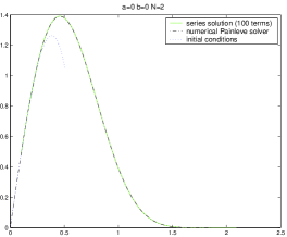
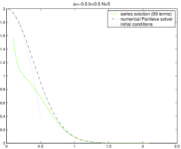
Figure 1. Plot of $\nu_{N}^{a+1/2,b+1/2}(\tfrac{\pi}{N}\theta)$, the scaled distribution of the first eigenvalue. On the left $N=2$, $a=0$ and $b=0$. The numerical solver was given the initial conditions (blue dotted line) and produced the solution shown with the dot-dashed line. This is indistinguishable from the series expansion (green solid line) using 100 terms. On the right $N=5$, $a=-0.5$ and $b=0.5$. The numerical solver was given the initial conditions (blue dotted line) and produced the solution shown with the dot-dashed line. The tail agrees with the series expansion (green solid line) using 99 terms. In both figures the numerical solver was run with values of $t_{0}=1-10^{-7}$, $\texttt{reltol}=10^{-5}$ and $\texttt{abstol}=10^{-6}$.

For values of $a>0$ the MATLAB solver breaks down. Trials with $a=0.001$ still work, but already $a=0.01$ fails to produce a good solution. Moving $t_{0}$ away from 1, for example to $1-10^{-2}$, helps achieve a better curve, but as can be seen from Figure 2, the initial conditions are not close enough to the true curve at this point to produce a valid solution. Decreasing reltol and abstol, even by a factor of 1000, does not make a visible difference to the curve. We note that unfortunately this means that while the MATLAB solver works very well for the group SO$(2N)$, we cannot use it to produce solutions for SO$(2N+1)$ and USp$(2N)$.

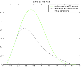
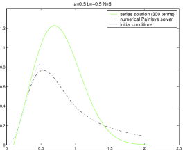
Figure 2. Plot of $\nu_{N}^{a+1/2,b+1/2}(\tfrac{\pi}{N}\theta)$, the scaled distribution of the first eigenvalue. On the left $N=2$, $a=0.5$ and $b=-0.5$. The numerical solver was given the initial conditions (blue dotted line) and produced the solution shown with the dot-dashed line. This fails to produce an accurate solution, as shown by comparison with the series expansion (green solid line) using 50 terms. On the right $N=5$, $a=0.5$ and $b=-0.5$. The numerical solver was given the initial conditions (blue dotted line) and produced the solution shown with the dot-dashed line. This fails to produce an accurate solution, as shown by comparison with the series expansion (green solid line) using 300 terms. The value of $t_{0}$ in the two plots are $t_{0}=1-7\times 10^{-2}$ and $t_{0}=1-10^{-2}$ respectively, and for both plots $\texttt{reltol}=10^{-7}$ and $\texttt{abstol}=10^{-7}$.

For $a>0$ and small values of $N$ a solution valid over the whole interval can still be glued together by matching the series solution (with a sufficient number of coefficients) for the tail and bulk of the curve with the known asymptotic behavior near $\phi=0$. The right-hand plot in Figure 2 shows that this is certainly possible for $N=5$.

The series solution produces a very accurate curve with only 50 terms when $N=2$, but the number of terms needed to obtain a solution which is meaningful over a large interval increases with $N$, which is to be expected because the most interesting behavior occurs near $\phi=0$ and can only be captured at the price of using many terms in an expansion about $\phi=\pi$. A good curve for $N=5$ requires around 300 terms. We did not produce results for higher $N$ as the run time was prohibitive, but on a fast computer more terms could be computed and good solutions for larger $N$ could be achieved by this method.

8. Summary

In summary, we find that our MATLAB code for numerically solving the nonlinear second-order differential equation (Painlevé VI) of the auxiliary Hamiltonian $h(t)$ associated to the $\tau$-function $\widetilde{E}_{N}^{(a,b)}(t)$, giving the distribution of the first level in a Jacobi ensemble $J_{N}^{{(a,b)}}$, appears to work fine for arbitrary $N$ provided the parameters lie in the ranges: $-0.5\leq a\leq 0$ and $-0.5\leq b\leq 0.5$. We restricted our tests to the interval $[-0.5,0.5]$ as this is the range of interest interpolating between the classical compact groups SO$(2N)$, SO$(2N+1)$ and USp$(2N)$. The program’s numerical accuracy is confirmed by comparing it with a power-series expansion of the solution found using SAGE. Unfortunately the restriction on $a$ to be non-positive means that the numerical solver cannot cope with the symplectic group USp$(2N)$ nor the odd orthogonal group SO$(2N+1)$. For positive $a$ and small values of $N$ this limitation can be overcome by using the series expansion to obtain the tail and the bulk of the distribution, matching the series result with the initial conditions for the behaviour near the origin. In a forthcoming paper our algorithms are applied to study the distribution of the first zero of $L$-functions with even functional equation associated with quadratic twists of a fixed elliptic curve. In the limit of large conductors in families of such $L$-functions the zero statistics are expected to be modelled by eigenvalues from SO$(2N)$.

Appendix A MATLAB Code

Here we give the MATLAB code for numerically solving the Painlevé VI equation associated to the distribution of the first eigenphase of random matrix ensembles in the Jacobi ensemble $J_{N}=J_{N}^{(\alpha,\beta)}$.

The main program is painleve6.m and it computes the numerical solution to the system of differential equations (3.8) for the Jacobi ensemble $J_{N}^{(a,b)}$. For fixed variables a, b, N the program is called by entering

(A.1) function [t,H,theta,Fp] = painleve6(a,b,N)

Here t, H correspond to the variables $t$ and $H$ (see (3.7)), and theta corresponds to the rescaled angular variable $\theta=N\phi/\pi={\frac{N}{\pi}}\cos^{-1}(2t-1)$. The output variable Fp in (A.1) is a vector of values of the rescaled distribution

(A.2) $$\nu_{N}^{(a+1/2,b+1/2)}\bigg{(}\frac{\pi\theta}{N}\bigg{)}=\frac{\pi}{2N}\sin\bigg{(}\frac{\pi\theta}{N}\bigg{)}\frac{\widetilde{E}_{N}^{(a,b)}(t)}{t(t-1)}\left[h(t)-te_{2}^{\prime}[{\rm\bf{b}}]+\tfrac{1}{2}e_{2}[{\rm\bf{b}}]\right]$$

of the first eigenphase (the rescaling achieves mean unit spacing of the $N$ eigenphases $\theta_{1},\dots,\theta_{N}$ on $[0,N]$), as obtained from (3.10) via the rescaled variable $\theta$ (= theta). The subsequent command

(A.3) plot(theta, Fp)

plots the distribution Fp (as defined in (A.2)) of the first rescaled eigenphase $\theta_{\min}$ for $J_{N}$. Notice that a=-0.5 and b=-0.5 corresponds to SO$(2N)$. Likewise setting a=0.5 and b=-0.5 gives SO($2N+1$) and finally USp$(2N)$ would correspond to choosing a=0.5 and b=0.5.

 

The code of painleve6.m is given as follows

function [t,H,theta,Fp] = painleve6(a,b,N)

t0 = 1 - 1e-7;
phi0 = acos(2*t0-1);

% in parameter regions where the numerical solver is robust t0 can be
% taken to be about 1-1e-7

  b1 = (a+b)/2+N;
  b2 = (a-b)/2;
  b3 = -(a+b)/2;
  b4 = -(a+b)/2-N;
  e2p = b1*b3 + b1*b4 + b3*b4;
  e2 = e2p + b2*(b1+b3+b4);
  r = a+0.5; % note that r and s correspond to alpha and beta
  s = b+0.5;

  % initial conditions below are from Section 5. The files Hone.m
  % and Htwo.m calculate often-used ratios of gamma functions.  EN,
  % ENderiv1 and ENderiv2.m calculate E_N^{(a,b)}(phi), and its
  % first and second derivatives with respect to phi
  % (*not* with respect to t).

  root0 = sqrt(t0*(1-t0));
  E0 = EN(r,s,N,phi0);
  E0d = ENderiv1(r,s,N,phi0);
  E0dd = ENderiv2(r,s,N,phi0);
  H0 = [ E0; ...
         t0*e2p - 0.5*e2 + root0*E0d/E0; ...
         e2p + (0.5-t0)/root0 * E0d/E0 - E0dd/E0 + (E0d/E0)^2 ];

  % First component of H will be   \tilde{E}_N^{(a,b)}(t)
  % Second component of H will be the auxiliary hamiltonion h(t)
  % Third component of H will be h’(t)
  % H0 contains the initial conditions at t=t0 (Note: t0 is a
  % number very close to 1, not close to zero!!

  opts=odeset(’reltol’,1e-5,’abstol’,1e-6);

  % a command like "opts=odeset(’reltol’,1e-5,’abstol’,1e-6);" works
  % fine for parameter ranges where the numerical solver is robust,
  % and the program just takes a few seconds/minutes to run.
  % As a becomes positive the differential equation
  % solver has trouble and we don’t get a correct solution
  % when N is large, a plot on a better scale is produced by
  % replacing the second argument in the range [t0,0.01] with
  % 0.5*cos(2*pi/N)+1/2

  [t,H] = ode45(@p6diff,[t0,0.01],H0,opts,b1,b2,b3,b4,e2p,e2);

  F = H(:,1);
  h = H(:,2);
  % theta is the scaled angular variable: theta=(N/pi)*acos(2*t-1)
  theta = (N/pi)*acos(2*t-1);

  % Fp(theta) is the distribution of the first eigenvalue in scaled
  % variables
  Fp = (pi/2/N)*sin(pi*theta/N).*F./t./(t-1).*(h-e2p*t+e2/2);

  The system (3.12) is defined in the file p6diff.m. The code is given as

function dH = p6diff(t,H,b1,b2,b3,b4,e2p,e2)
dH = zeros(3,1);
dH(1) = H(1)/t/(t-1)*(H(2)-e2p*t+e2/2);
dH(2) = H(3);
dH(3) = +sqrt( ...
              ( ...
               (H(3)+b1^2)*(H(3)+b2^2)*(H(3)+b3^2)*(H(3)+b4^2) ...
               - ( H(3)*(2*H(2)-(2*t-1)*H(3)) + b1*b2*b3*b4 )^2 ...
              ) / H(3) ...
             ) /t/(1-t);

 

The often used ratios of gamma functions $H_{1}$ and $H_{2}$ (see (5.2) and (5.3)) are coded in the files Hone.m and Htwo.m given as

function H1 = Hone(r,s,N)
H1 = gamma(r + N +0.5) * gamma(r + s + N) / 2^(2*r) ...
     / gamma(N + 1) / gamma(r + 1.5) / gamma(r + 0.5) ...
     / gamma(s + N - 0.5);

and

function H2 = Htwo(r,s,N)
H2 = gamma(r + N + 0.5) * gamma(r + s + N + 1) / 2^(2*r+ 1) ...
     / gamma(N + 1) / gamma(r + 2.5) / gamma(r + 0.5) ...
     / gamma(s + N - 0.5);

 

Finally, we provide the code for EN.m, ENderiv1.m, and ENderiv2.m

function E = EN(r,s,N,phi)
% This is an expansion in phi around phi=0 of E_N^{(a,b)}(phi).

% See (5.1).

exponent = 2*r+1;
E = 1;
E = E - N*Hone(r,s,N)*phi.^exponent/exponent;
exponent = exponent + 2;
E = E + N*( ...
           (N-1)*Htwo(r,s,N)*phi.^exponent ...
           + (r/12.0+s/4)*Hone(r,s,N)*phi.^exponent ...
          )/exponent;


function Ed = ENderiv1(r,s,N,phi)
% This is \frac{d}{d\phi}E_N^{(a,b)}(phi).

% See (5.4).

exponent = 2*r;
Ed = -N*Hone(r,s,N)*phi.^exponent;
exponent = exponent + 2;
Ed = Ed + N*( ...
              (N-1)*Htwo(r,s,N)*phi.^exponent ...
              + (r/12.0+s/4)*Hone(r,s,N)*phi.^exponent ...
            );


function Edd = ENderiv2(r,s,N,phi)
% This is \frac{d}{d\phi}E_N^{(a,b)}(phi).

% See (5.5).

exponent = 2*r-1;
Edd = -2*r*N*Hone(r,s,N)*phi.^exponent;
exponent = exponent+2;
Edd = Edd ...
      + N*(exponent+1)*( ...
                         (N-1)*Htwo(r,s,N)*phi.^exponent ...
                         + (r/12.0+s/4)*Hone(r,s,N)*phi.^exponent ...
                        );

Appendix B SAGE Code

Below follows the SAGE code implementing the symbolic power series evaluation of the $\tau$-function. Note that the parameters $a,b,N$ correspond to a, b, N, which along with DEGREE (the degree of the sought-after truncation of the power series) are hard-coded in the first four lines. Note also that the code provided only works for rational values of $a,b$ and integer $N$ (cf., Section 6). Once run, the code defines functions E(t), Ep(t), pcummul(phi) and nu(phi) implementing $\widetilde{E}_{N}^{(a,b)}(t),\frac{d}{dt}{\widetilde{E}_{N}^{(a,b)}}(t),1-E_{N}^{(\alpha,\beta)}(\phi)$ and $\nu(\phi)$, respectively. In particular, nu has been used to produce the plots in figures 1 and 2.

Note that in Python syntax any text following the literal # is simply a comment.

⬇

1DEGREE = 50 # degree (plus 1) of the truncated power series

2a = -1/2

3b = -1/2

4n = 4

5

6b1 = (a+b)/2+n

7b2 = (a-b)/2

8b3 = -(a+b)/2

9b4 = -(a+b)/2-n

10e2p = b1*b3 + b1*b4 + b3*b4

11e2 = e2p + b2*(b1+b3+b4)

12

13R.<x> = QQ[’x’] # R = Q[x]

14S.<t> = PowerSeriesRing(R,default_prec=DEGREE)

15 # S = Q[x][[t]]

16def Jac(a,b,n):

17 jac=1.

18 for i in xrange(n):

19 jac *= real(gamma(a+i+1.)) * real(gamma(b+i+1.))\

20 * real(gamma(i+2.)) / real(gamma(a+b+n+i+1.))

21 return jac

22# NOTE: Jac (as above) only works for *integer* values of n

23

24leadcoef = Jac(0,b,n)/Jac(a,b,n)

25leadexp = n*(n+b)

26g = [-e2/2-leadexp, e2p+leadexp*(1+a/(b+2*n))]

27h = g[0] + t*g[1]

28

29X = var(’X’) # symbolic Maxima variable

30

31# BEGIN MAIN LOOP: Finds successive coefficients of series h(t)

32for i in xrange (2,DEGREE):

33 h = h + x*t^i + O(t^(i+2))

34 hp = h.derivative()

35 hpp = hp.derivative()

36 PEZ = hp*(hpp*t*(1-t))^2 + (hp*(2*h-hp*(2*t-1))+b1*b2*b3*b4)^2 \

37 - (hp+b1^2)*(hp+b2^2)*(hp+b3^2)*(hp+b4^2)

38 LHS = PEZ[i](X) # Substitute x=X in p_i(x)

39 solucion = solve (LHS==0, X) # Find root of p_i(X)

40 g.append(QQ(solucion[0].rhs())) # The root becomes

41 # the next coefficient

42 # Now reconstruct h up to degree i using the newly-found g[i]

43 h = g[0]+g[1]*t+g[2]*t^2

44 for j in xrange (3,i+1):

45 h += g[j]*t^j

46 # END OF MAIN LOOP

47

48h = h + O(t^DEGREE)

49

50h1 = (h-h[0])/t

51F = h1

52F -= e2p+leadexp

53F /= t-1+O(t^DEGREE)

54F = F.integral()

55F = F.exp()

56F = F.truncate(DEGREE+1)

57

58htilde = h1 - e2p

59htilde = htilde.truncate(DEGREE-1)

60

61def E(u):

62 return leadcoef * u^leadexp * F(u)

63def Ep(u):

64 return (htilde(u)/(u-1) + leadexp/u/(1-u)) * E(u)

65

66def pcummul(theta):

67 return 1-E((1+cos(theta))/2)

68def nu(theta):

69 if theta < 1.e-6 or theta > pi - 1.e-6:

70 return 0

71 t = (1+cos(theta))/2

72 return sqrt(t*(1-t)) * Ep(t)

References

- [1] Y. Chen and L. Zhang. Painlevé VI and the unitary Jacobi ensembles. Stud. Appl. Math., 2010, DOI: 10.1111/j.1467-9590.2010.00483.x.
- [2] D. Dai and L. Zhang. Painlevé VI and Hankel determinants for the generalized Jacobi weight. J. Phys. A, 43(5):055207, 2010.
- [3] E. Dueñez. Random matrix ensembles associated to compact symmetric spaces. Comm. Math. Phys., 244(1):29–61, 2004.
- [4] A. Edelman and P. Persson. Numerical Methods for Eigenvalue Distribution of Random Matrices. math-ph/0501068, preprint, 2005.
- [5] P. J. Forrester and N. S. Witte. Application of the -function theory of Painlevé equations to random matrices: PVI, the JUE, CyUE, cJUE and scaled limits. Nagoya Math. J., 174:29–114, 2004.
- [6] P. J. Forrester and N. S. Witte. Random matrix theory and the sixth Painlevé equation. Journal of Physics A, 39, 2006.
- [7] Peter J. Forrester. Log-Gases and Random Matrices. Number 34 in London Mathematical Society Monographs. Princeton University Press, 2010.
- [8] N.M. Katz and P. Sarnak. Random Matrices, Frobenius Eigenvalues, and Monodromy. AMS Colloquium Publications, 1999.
- [9] N.M. Katz and P. Sarnak. Zeros of zeta functions and symmetry. Bull. Amer. Math. Soc., 36:1–26, 1999.
- [10] Maxima, a Computer Algebra System. Open source software. http://maxima-project.org.
- [11] M.L. Mehta. Random Matrices. Academic Press, 2nd edition, 1991.
- [12] S.J. Miller. One- and two-level densities for rational families of elliptic curves: evidence for the underlying group symmetries. Compos. Math., 140:952–992, 2004.
- [13] S.J. Miller. Investigations of zeros near the central point of elliptic curve -functions. Experiment. Math., 15 (3):257–279, 2006. (E-print: math.NT/0508150).
- [14] Clarkson P.A., Mazzocco M. Joshi N., Nijhoff. F. W., and Noumi M. One hundred years of PVI, the Fuchs-Painlevé equation. Journal of Physics A, 39, 2006.
- [15] Christian Robert and George Casella. Monte Carlo Statistical Methods (Springer Texts in Statistics). Springer-Verlag, second edition, 2004.
- [16] SAGE. Open source mathematics software. http://www.sagemath.org.
- [17] M. P. Young. Low-lying zeros of families of elliptic curves. J. Amer. Math. Soc., 19:205–250, 2006.