Supernova Remnants as a Probe of Dust Grains in the Interstellar Medium

Abstract

The Ph.D. Thesis of Brian J. Williams, submitted to and accepted by the Graduate School of North Carolina State University. Under the direction of Stephen P. Reynolds and Kazimierz J. Borkowski.

Interstellar dust grains play a crucial role in the evolution of the galactic interstellar medium (ISM). Despite its importance, however, dust remains poorly understood in terms of its origin, composition, and abundance throughout the universe. Supernova remnants (SNRs) provide a laboratory for studying the evolution of dust grains, as they are one of the only environments in the universe where it is possible to observe grains being both created and destroyed. SNRs exhibit collisionally heated dust, allowing dust to serve as a diagnostic both for grain physics and for the plasma conditions in the SNR. I present theoretical models of collisionally heated dust which calculate grain emission as well as destruction rates. In these models, I incorporate physics such as nonthermal sputtering caused by grain motions through the gas, a more realistic approach to sputtering for small grains, and arbitrary grain compositions porous and composite grains. I apply these models to infrared and X-ray observations of Kepler’s supernova and the Cygnus Loop in the galaxy, and SNRs 0509-67.5, 0519-69.0, and 0540-69.3 in the LMC. X-ray observations characterize the hot plasma while IR observations constrain grain properties and destruction rates. Such a multi-wavelength approach is crucial for a complete understanding of gas and dust interaction and evolution. Modeling of both X-ray and IR spectra allows disentangling of parameters such as pre and postshock gas density, as well as swept-up masses of gas and dust, and can provide constraints on the shock compression ratio. Observations also show that the dust-to-gas mass ratio in the ISM is lower by a factor of several than what is inferred by extinction studies of starlight. Future observatories, such as the James Webb Space Telescope and the International X-ray Observatory, will allow testing of models far beyond what is possible now.

1 Introduction to Supernovae and Supernova Remnants

Supernova explosions are among the most energetic events in the universe since the Big Bang, releasing more energy ($\sim 10^{51}-10^{53}$ ergs) than the Sun will release over its entire lifetime. They are the cataclysmic ends of certain types of stars, and are responsible for seeding the universe with the material necessary to form other stars, planets, and life itself. We owe our very existence to generations of stars that lived and died billions of years ago, before the formation of our Sun and solar system. The processes of stellar evolution continue to occur today, with typical galaxies like the Milky Way hosting several supernovae per century, on average. The study of supernovae and the role they play in shaping the evolution of star systems and galaxies is truly an exploration of our own origins. Supernova remnants (SNRs), the expanding clouds of material that remain after the explosion, spread elements over volumes of thousands of cubic light-years, and heat the interstellar medium through fast shock waves generated by the ejecta from the star.

1.1 Stellar Evolution

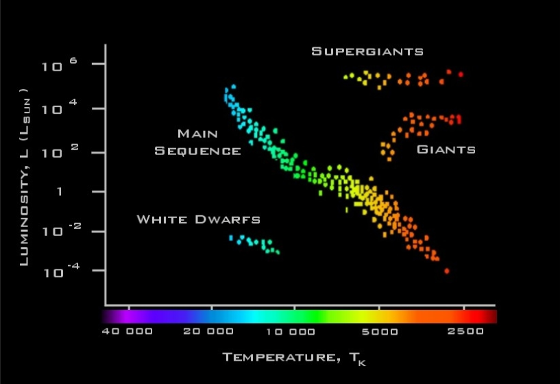
Figure 1.1: Hertzsprung-Russell Diagram, showing the temperatures of stars vs. luminosity. Taken from http://www.le.ac.uk/ph/faulkes/web/stars/o_st_overview.html.

Any study of SNRs must begin with the processes which cause a star to go supernova. Stars come in all sizes and colors (where the color of a star is related to its temperature), but virtually all stars live out their lives in a similar fashion. They spend the majority of their lives fusing hydrogen in their cores into helium, a process which releases energy. This process is not particularly efficient in stars; nevertheless, the sheer mass of available material to burn means that stars shine at a roughly constant brightness for millions, billions, even tens of billions of years. The life expectancy of a star is a rather sensitive function of its initial mass. This relationship is perhaps counterintuitively inverted, such that the more massive a star is, the shorter its lifetime. (This is due to the fact that massive stars, while having much more fuel to burn, fuse it at a much faster rate than do low-mass stars). Stars that are on the hydrogen burning phase of their lives are said to be on the “main sequence,” a reference to the Hertzsprung-Russell diagram seen in Figure 1.1.

This fusion process that takes place in the stellar core is one-half of a balancing act, providing the internal pressure to support the star against the other half, gravity. This cosmic “tug-of-war” can only last as long as the star has fuel to burn; once the hydrogen fuel in the core is depleted, gravity will pull the star in on itself unless a new process can provide the necessary counter-balancing force. The fate of a star at this point depends on its mass, with high and low-mass stars following very different paths.

1.1.1 Low-Mass Stars

Stars that begin their main-sequence lives with a mass of less than about 8 solar masses ($M_{\odot}$, where $M_{\odot}$ is $\sim 1.99\times 10^{33}$ grams) will spend the majority of their lives in the hydrogen burning phase. When their hydrogen runs out, they will swell into red giants, increasing in volume by a factor of $>$ 1000. (The smallest of stars, with masses $<$ 0.5 $M_{\odot}$, will not even have enough power to reach this stage). The red giant phase is typically characterized by a helium core surrounded by a hydrogen burning shell. When the core contracts and heats to temperatures above $\sim 10^{8}$ K, helium burning will begin, fusing helium to carbon via the triple-alpha process. The core of the star that remains typically cannot fuse much beyond carbon and oxygen, and collapses further when the helium supply is used up. The outer layers of the star are ejected, creating the misleadingly named “planetary nebula.” Collapse continues until the degenerate pressure of electrons in the plasma is sufficient to balance the gravitational forces, creating a “white dwarf” star. A typical white dwarf has a mass of $\sim 0.6-0.7M_{\odot}$ contained in a volume about the size of the Earth (R $\sim 6000$ km), which leads to an average density for a white dwarf of $\sim 10^{6}$ g cm^-3. White dwarfs are typically very stable (although see section 1.2), and will exist as burned-out remnants of once bright stars indefinitely.

1.1.2 High-Mass Stars

Stars above $\sim 8$ $M_{\odot}$ are hot enough at their cores to fuse hydrogen into helium, helium into carbon, carbon into oxygen, neon, silicon, sulfur and other elements, stepping up the periodic table. Once iron (element 26) is reached, though, it no longer becomes energetically favorable for the fusion process to continue. The iron core collapses in upon itself on timescales of the order of a second, sidestepping electron degeneracy pressure by eliminating electrons, combining them with protons to form neutrons. Once nuclear density ($\sim 10^{15}$ g cm^-3) is reached, the degeneracy pressure of neutrons is sufficient to halt the collapse, and the core becomes a proto-neutron star. The remaining infalling material from the core bounces off of this now hard core, ejecting the outer layers of the star in a fantastic explosion known as a “core-collapse supernova.” The proto-neutron star forms a neutron star, a stellar remnant of order 1 $M_{\odot}$ and R $\sim 10$ km, with an average density of $\sim 10^{15}$ g cm^-3. For highly massive stars, it is possible that even neutron degeneracy pressure cannot halt the collapse of the core, and a stellar-mass black hole is formed.

1.2 Supernova Classification

As in many sciences, observations of events or objects in astronomy often precede theoretical explanations for said events. However, unlike in most disciplines, astronomers normally do not have the means to conduct laboratory tests of observed phenomena. This often leads to a significant time delay between the observation of and the theoretical description of a given event. As a result, the field is riddled with examples of “historical inaccuracies” when it comes to naming and classification schemes. A prime example of this is the supernova classification scheme, where astronomers classify supernovae as “Type I” or “Type II” based solely on the existence of hydrogen lines in their spectra; Type I SNe show no hydrogen lines, Type II do. It was only later realized that vastly different processes can be responsible for this bit of observational data.

1.2.1 Type Ia

The vast majority of stars in the galaxy are $<8M_{\odot}$, meaning (see Section 1.1.1) that they are destined to end their lives as white dwarfs. However, many stars in the galaxy are also part of binary (or even triple) systems. If a white dwarf is contained in a binary system with a companion star that enters its red giant phase (or has even slightly evolved off the main sequence), and the separation between the stars is sufficiently close, the white dwarf can gravitationally strip matter from its companion. Mass transfer occurs between the two stars, with the white dwarf growing in mass via an accretion disk. White dwarfs can only exist up to the “Chandrasekhar limit,” and a white dwarf pushed over this limit ($\sim 1.4M_{\odot}$) will become unstable, igniting a deflagration, or subsonic burning, of material in the star. This deflagration will lead to a detonation, a supersonic thermonuclear explosion of the entire white dwarf. The entire 1.4 $M_{\odot}$ of material is ejected into the surrounding medium at speeds of $\sim 10,000$ km s^-1, releasing about 10⁵¹ ergs of kinetic energy. Type Ia SNe leave behind no compact remnant, and their light curve, i.e. the brightness of the supernova as a function of time, is primarily powered by the radioactive decay chain of nickel-56 to cobalt-56 to iron-56. Their light curves peak a few days after explosion, then slowly fade over the course of a few months. Since all white dwarfs are thought to explode at an identical mass via the same mechanism, their light curves are quite similar in peak brightness, and can be used as a “standard candle” to determine extragalactic distances. Type Ia spectra show no hydrogen because white dwarfs are made mostly of carbon and oxygen, nearly all of which is burned to nickel in the explosion.

1.2.2 Type II

Type II supernovae result from the deaths of massive stars, greater than 8 $M_{\odot}$, but generally not more than $\sim 25-30M_{\odot}$. These stars end their lives as core-collapse SNe (CCSNe), ejecting their outer layers (5-25 $M_{\odot}$) at a velocity of $\sim 5,000-10,000$ km s^-1. Coincidentally, they yield roughly the same amount of kinetic energy ($\sim 10^{51}$ ergs) as do type Ia SNe, but their overall energetics are much greater. Ninety-nine percent of the energy released in a CCSN is carried off by neutrinos. Type II SNe leave behind a neutron star that is typically $\sim 1.4M_{\odot}$ with an initial temperature (kT) of several MeV. Type II SNe can be further divided into subclasses based either on the shape of the light curve or the spectrum (e.g. IIP, IIL, IIb, IIn, etc.). They show hydrogen lines in their spectra because the outer atmosphere of the star at the time of explosion still contained a significant amount of hydrogen.

1.2.3 Type Ib and Ic

Type Ib and Ic SNe are also the result of a core-collapse event, differing from type II in that they do not show hydrogen lines in their spectra. The physical reason behind this is that type Ib and Ic SNe result from stars that have shed their outer layers via stellar winds (“Wolf-Rayet” stars) or gravitational interaction with a companion star prior to explosion. Type Ib explosions result from stars that have lost only their hydrogen envelope; type Ic from stars that have lost both their hydrogen and helium envelopes. Type Ib and Ic SNe are believed to be the result of stars with a progenitor mass of $\mathrel{\hbox to0.0pt{\lower 4.0pt\hbox{\hskip 1.0pt$\sim$}\hss}\raise 1.0pt\hbox{$>$}}30M_{\odot}$, although this number could be lower in binary systems. They leave behind neutron stars and stellar-mass black holes. As with type II SNe, most of their energy is carried off in neutrinos, and their light-curves, both in peak brightness and in shape, can vary greatly.

1.3 Astrophysical Shocks

Shock waves, propagating supersonic disturbances, occur commonly in all sorts of astro-environments throughout the universe, where conditions are unlike those found on Earth. Densities in the interstellar medium (ISM) are on the order of a few particles per cubic centimeter, six orders of magnitude less than can be produced in the best laboratory vacuum systems. Sound speeds in the ISM are usually on the order of a few km s^-1, relatively slow by astrophysical standards. The shock waves generated by a supernova are an excellent example of a strong shock, with shock speeds often being several thousand times the speed of sound in the ISM. These shock waves compress, sweep, and heat interstellar material. In fact, supernova shock waves are one of the main sources of heating of the interstellar medium, as well as the mechanism for distributing material throughout the universe.

The following is a mathematical description of a shock wave, beginning with the Rankine-Hugoniot Conditions, given by

$$\rho_{1}v_{1}=\rho_{2}v_{2},$$ (1)

$$\rho_{1}v_{1}^{2}+p_{1}=\rho_{2}v_{2}^{2}+p_{2},$$ (2)

$$\frac{1}{2}v_{1}^{2}+E_{1}+\frac{p_{1}}{\rho_{1}}=\frac{1}{2}v_{2}^{2}+E_{2}+\frac{p_{2}}{\rho_{2}},$$ (3)

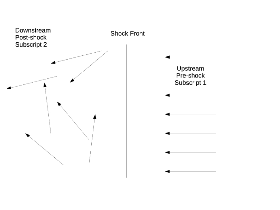
Figure 1.2: Shockwave diagram, in the frame of reference of the shock. Arrows represent the velocities of particles upstream and downstream of the shock. In this frame, upstream material (at rest in the observer’s frame) races in towards the shock. The shock then randomizes the velocities of the particles, and gives them a bulk velocity downstream of 1/4 their initial velocity (for a strong shock with $\gamma=5/3$).

where $\rho$ is the density of the gas, $v$ is the velocity, $p$ is the thermal pressure, and $E$ is the internal energy, given by $dW=dE=-p$d$V$. Subscript 1 denotes pre-shock material (that is, ambient interstellar material that is ahead of the expanding shock wave) and 2 denotes post-shock gas. These equations are written in the frame of reference of the shockwave (see Figure 1.2). In particular, this means that $v_{1}$ is not zero (in fact, $v_{1}=-v_{shock}$) even though there is no motion in front of the shock in the observer’s frame.

Equation (1) is the conservation of mass across the shock, while Equation (2) shows that the sum of the ram pressure, $\rho v^{2}$, and thermal pressure $p$ must be equal across the shock. This amounts to a conservation of momentum. Equation (3) is the conservation of energy (kinetic, internal, and thermal).

The volume of the gas is given by $V$, such that d$V=$d$\frac{1}{\rho}$. Thus $dE=-p$d$V=-K\rho^{\gamma}$d$\frac{1}{\rho}$, which can be integrated to obtain $E=\frac{1}{\gamma-1}\frac{p}{\rho}$. The thermodynamic relation between pressure and density is $p=K\rho^{\gamma}$ where $K$ is a constant (although it is not constant across the shock) and $\gamma$ is the polytropic index of the gas. $\gamma$ varies depending on the properties of the fluid and is given by:
$\gamma=5/3$ for non-relativistic monoatomic gas (as is generally found in the ISM),
$\gamma=4/3$ for relativistic monoatomic gas,
$\gamma=7/5$ for non-relativistic diatomic gas.

Using this, eq. (3) becomes

$$\frac{1}{2}v_{1}^{2}+\frac{1}{\gamma-1}\frac{p_{1}}{\rho_{1}}=\frac{1}{2}v_{2}^{2}+\frac{1}{\gamma-1}\frac{p_{2}}{\rho_{2}}$$ (4)

Using the Rankine-Hugoniot conditions, it can be shown that

$$\frac{\rho_{2}}{\rho_{1}}=\frac{(\gamma+1)p_{2}+(\gamma-1)p_{1}}{(\gamma+1)p_{1}+(\gamma-1)p_{2}}=\frac{v_{1}}{v_{2}}.$$ (5)

This is the shock jump condition for density, giving the compression ratio, which relates density (and thus fluid velocity) ahead of the shock and behind the shock. In the limit of strong shocks, that is, $p_{2}\gg p_{1}$, or $M\gg 1$, where $M$ is the Mach number (defined as $v_{shock}/v_{sound}$), we can neglect the pre-shock pressure so that

$$\frac{\rho_{2}}{\rho_{1}}=\frac{\gamma+1}{\gamma-1}=4$$ (6)

for $\gamma=5/3$. In the limit of a strong shock, we also have

$$\frac{p_{2}}{p_{1}}=\frac{2\rho_{1}v_{1}^{2}}{p_{1}(\gamma+1)},$$ (7)

or

$$p_{2}=\frac{2\rho_{1}v_{1}^{2}}{\gamma+1}.$$ (8)

The gas is also governed by the ideal gas law such that $p_{2}=n_{2}kT_{2}$, where k is Boltzmann’s constant. So

$$p_{2}=\frac{2\rho_{1}v_{1}^{2}}{\gamma+1}=\frac{3}{4}\rho_{1}v_{1}^{2}=n_{2}kT_{2},$$ (9)

where $n=\frac{\rho}{m}$ = total particle number density, and $m$ is the mean mass per particle. Thus,

$$p_{2}=\frac{2\rho_{1}v_{1}^{2}}{\gamma+1}=\frac{3}{4}\rho_{1}v_{1}^{2}=\frac{\rho_{2}}{\mu m_{p}}kT_{2},$$ (10)

where $m_{p}$ is the mass of a proton, equal to $1.67\times 10^{-24}$ grams. Further simplifying, we have

$$kT_{2}=\frac{3}{16}\mu m_{p}v_{s}^{2},$$ (11)

where $\mu m_{p}$ is the mean mass per particle behind the shock (for a fully ionized plasma of cosmic abundances, $\mu\sim 0.6$). This is the temperature behind a shock, where $v_{s}=v_{1}$ is the shock speed. $kT_{2}$ is the “shock temperature,” which is the average of proton and electron temperatures. In the absence of heating of electrons at the shock (and assuming no sharing of energy between protons and alpha particles), the initial temperature ratio between protons and electrons, $T_{p}/T_{e}$, is just the ratio of the masses of protons and electrons, $m_{p}/m_{e}$ = 1836. Behind the shock, these temperatures equilibrate to bring down $T_{p}$ and bring up $T_{e}$, but the timescale for equilibration is long, and is a function of the post-shock temperature and density. Observationally, it is known (Ghavamian et al., 2001) that an inverse correlation exists between shock speed and degree of equilibration of protons and electrons at the shock, with near full equilibration seen in old remnants like the Cygnus Loop ($v_{s}$ $\sim 300-400$ km s^-1) and little equilibration seen in younger remnants like Tycho ($v_{s}$ $\sim 2000$ km s^-1).

For supernova shock waves of order a few thousand km s^-1, this shock temperature will be of order 10 million K. Thus, shocked gas will radiate thermal emission at X-ray energies, however, other emission mechanisms also operate in SNRs. Non-thermal emission from synchrotron radiation is often seen near the forward edge of the shock wave in young SNRs, and line emission from ionized elements is common in the shocked ejecta. Shocks in SNRs are “collisionless,” in that collisions between particles are extremely rare, meaning that particle interactions are mediated by magnetic fields. This is a good approximation when the Coulomb mean free path is much greater than the gyroradius of the thermal particles.

1.4 Supernova Remnants

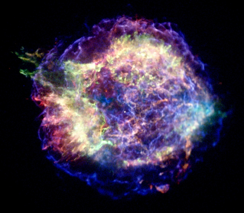
Figure 1.3: SNR Cassiopeia A, seen in X-rays from the Chandra X-ray Observatory. Image from http://chandra.harvard.edu/photo/2006/casa/

The expanding material ejected from the star, rich in heavy elements like oxygen, silicon, and iron, as well as the shock wave which it drives into the ISM is known as a supernova remnant (SNR). Figure 1.3 shows Cassiopeia A, an example of a young ($\sim 330$ yrs) SNR in our own galaxy. Although Cassiopeia A is known to have resulted from a CCSN, it is generally difficult to tell the type of SN only by looking at the remnant. SNRs remain visible for thousands, often tens or hundreds of thousands of years before dissipating their energy into the ISM. The life of a SNR can be thought of as consisting of four phases.

1.4.1 Free Expansion Phase

Immediately following the explosion, the ejecta from the supernova race out into the ISM at speeds of $\sim 10,000$ km s^-1, driving a strong shock at the leading edge. Since the ejected mass is significantly greater than the mass of the rarefied medium it encounters, there is no appreciable slowing of the ejecta by the ambient medium. How long this phase lasts depends on both the ejected mass of the SN and the density of the CSM in front of the shock, and can be anywhere from a few days to years.

1.4.2 Reverse-Shock Phase

As the shock continues to expand and sweep material it encounters, the accumulated mass becomes non-negligible, and gradually causes the shock to slow. The ejecta behind the shock, however, are still traveling at a free-expansion velocity, and slam into the decelerating material ahead of it. This causes a reverse shock to form. Initially, this “reverse” shock moves inward only in the Lagrangian shock frame, and still moves outward in the observer’s frame. The reverse shock, however, eventually “turns around” and moves inward in the frame of reference of the observer. It typically takes of order hundreds of years for this transition to occur. When the ejecta are in free-expansion cooling is almost entirely adiabatic. While this adiabatic cooling is effective in lowering the temperature of the ejecta, energy is still conserved for the system because the energy is not radiated away. Upon encountering the reverse shock the ejecta are heated, like the ISM at the forward shock, to very high temperatures, thus radiating strongly in X-rays. This radiative cooling is still relatively inefficient, and most of the energy of the SNR+ISM system is conserved. The duration of the reverse shock phase can last tens to thousands of years.

1.4.3 Sedov-Taylor Phase

Once the mass swept-up by the forward shock greatly exceeds the ejecta mass, the remnant enters the Sedov-Taylor phase (often known simply as the Sedov phase). The reverse shock has propagated all the way back through the ejecta and dissipated, and the remnant can be described by a self-similar solution (Sedov 1959). The similarity variable can be derived by dimensional analysis, and is given by

$$\xi=R(\rho/Et^{2})^{1/5}$$ (12)

where $R$ is the distance the blast wave has traveled from the supernova, $E$ is the explosion energy of the initial event, $\rho$ is the density of the ISM, and $t$ is time. $\xi$ is dimensionless, and equation 12 can be used to show that the distance traveled by the blast wave (for $\gamma=5/3$) as a function of $E$, $\rho$, and $t$, is given by

$$R\propto(\frac{E}{\rho})^{\frac{1}{5}}t^{\frac{2}{5}}.$$ (13)

It can be immediately seen from this that the shock velocity is given by

$$V_{s}=\frac{dR}{dt}=\frac{2R}{5t}.$$ (14)

The Sedov phase lasts for thousands to tens of thousands of years after the explosion.

1.4.4 Radiative Phase

The shock continues to sweep up material and decelerate, eventually reaching a point where the forward shock speed is only a few hundred km s^-1. At this point, the temperature of the post-shock gas drops below 10⁶ K, and radiative cooling of the gas becomes important. Cooling of the gas is a runaway process, as the more it cools, the more the cooling rate increases. As the gas temperature drops further, the material once again becomes visible in optical radiation. The forward shock is driven mostly by momentum conservation at this point, and eventually will turn sub-sonic and dissipate into the ISM.

1.5 Radiation Mechanisms in SNRs

SNRs radiate throughout the electromagnetic spectrum. In radio waves, the emission is entirely non-thermal in origin, resulting from synchrotron radiation from relativistic electrons spiraling around magnetic fields. Synchrotron emission is characterized by a featureless power-law spectrum, where the radio flux, $S_{\nu}$ is given by $S_{\nu}\propto\nu^{-\alpha}$, where $\nu$ is the frequency and $\alpha$ is the spectral index, which depends on the energy distribution of the electron population.

The primary focus of this work is on infrared (IR) emission from SNRs, the physical basis for which is described in Chapter 2. Briefly, IR emission is dominated by thermal continuum from warm dust grains, heated by collisions with the hot ions and electrons in the post-shock region. Remnants in the radiative phase can show IR line emission as well, from low to moderately ionized states of abundant heavy elements like O, Ne, S, Si, Ar and Fe.

At optical wavelengths, radiation prior to the radiative phase comes primarily from hydrogen Balmer lines (transitions from $n\geq 3\to 2$), such as H$\alpha$, $\lambda$ = 656.3 nm, and H$\beta$, $\lambda$ = 486.1 nm. This requires the presence of neutral hydrogen ahead of the shock, which is much more easily attained in the case of a type Ia SN, since CC SNe generally ionize the surrounding medium, either with ionizing radiation from the progenitor, or a flash of ultraviolet (UV) radiation at the moment of explosion. Charge exchange between slow neutral atoms and fast protons behind the shock produces fast-moving neutral atoms, generating a broad H$\alpha$ line, with a narrow component arising from stationary neutral atoms in the post-shock medium. During the radiative phase, strong optical lines are seen from a variety of atomic species, most strongly from H$\alpha$ and singly-ionized sulfur ([S II]). Ultraviolet (UV) emission from SNRs is also produced, generally from higher ionization states than in optical.

Soft X-rays (0.1-2 keV) are generally thermal in origin, and in SNRs are often dominated by line emission from highly ionized elements. Typically, elements that emit X-ray line emission have been stripped of all but one or two electrons, making them “hydrogen-like” or “helium-like.” As with optical and infrared lines, downward transitions of electrons to lower energy levels causes emission of a photon whose energy is equal to the transition energy between the electron’s bound states. For elements that still contain multiple electrons, the transitions between energy states become more complicated, and generally generate numerous lines which are smeared together by current X-ray spectroscopic technology. Continuum emission, detailed below, is also observed at these energies.

Hard X-rays (2-50 keV) in SNRs can be either thermal or non-thermal in origin. Thermal X-rays are dominated by continuum emission, although lines from K-shell electron transitions do exist beyond 2 keV for elements such as Si, S, Ar, and Fe. Thermal continuum seen in X-ray spectra is generally thermal Bremsstrahlung (also known as “free-free” emission), which occurs when electrons and protons interact. This process causes the electron to slow down, and energy conservation requires emission of a photon to account for the lost kinetic energy of the particle. Free-bound emission (or radiative recombination) can also take place when a proton or ion captures a free electron, emitting in the process a photon whose energy depends on both the free kinetic energy of the electron and the orbital to which it is captured.

Non-thermal emission in SNRs arises from synchrotron emission identical to that seen in radio waves, but from much more energetic electrons. The maximum photon energy in keV of an electron with energy $E$ is given by

$$h\nu=1.93(E/100TeV)^{2}(B/10\mu G)keV.$$ (15)

In order to produce synchrotron emission in the 2-10 keV range, electrons with energies of 100-200 TeV are required. Because this is well beyond the particle thermal energies for even a fast shock, another process must accelerate particles to high energies in remnants where non-thermal emission is conclusively identified. The origin of these high-energy cosmic-ray electrons is discussed in the next section.

At gamma-ray energies, emission can be produced by one of three processes; two of which are leptonic in origin, one of which is hadronic. Bremsstrahlung, both thermal and non-thermal in origin, can account for photons of all energies, up to TeV emission. Inverse-Compton scattering from relativistic electrons off of cosmic microwave background or far-infrared photons can upscatter the photons to very high energies. The only known hadronic source of gamma-ray emission is the decay of neutral pions, or $\pi^{0}$ particles, into two gamma-ray photons. This process occurs 98.7% of the time in $\pi^{0}$ decays. The $\pi^{0}$ particles themselves are produced in collisions between cosmic-ray protons and thermal protons, as well as protons and alpha particles in the pre-shock gas. The minimum pion energy required to produce a gamma-ray of energy $E_{\gamma}$ is given by

$$E_{min}(\pi)=E_{\gamma}+(m_{\pi}^{2}c^{4}/4E_{\gamma})$$ (16)

To produce high energy gamma rays ($>1$ GeV), the last term on the right becomes negligible, and the minimum pion energy needed is roughly equal to the gamma-ray energy observed.

It is likely that all of these processes play a role in the gamma-ray emission observed from SNRs. For a thorough review of SNRs at high energies, see Reynolds (2008).

1.6 Cosmic-Ray Acceleration in SNRs

Cosmic-rays are highly energetic particles, typically protons, alpha particles, and nuclei of heavier elements, with a small percentage of the population consisting of electrons, streaming through space at relativistic speeds. They can either be detected directly (at lower energies), or indirectly through interactions with atoms in the Earth’s upper atmosphere (at high energies). Upon the collision of a cosmic-ray with our atmosphere, a shower of particles (mostly containing pions) is produced. These pions decay further into electrons, positrons, muons, neutrinos, and photons, and can be detected from ground-based Cherenkov telescopes. Such telescopes can even reconstruct the events to determine the location in the sky from which the cosmic-ray came. Unfortunately, this location is not indicative of the original source of the particle. Since cosmic-rays are charged particles, they gyrate around the magnetic field lines of our Galaxy, and are essentially randomized by the time they reach Earth. This leads to a mystery: from where do cosmic-rays come?

1.6.1 Cosmic-Ray Sources

The fact that synchrotron emission is observed in radio waves for every Galactic SNR known shows that, at the very least, electrons are efficiently accelerated to energies of a few GeV. If electrons are accelerated, protons and ions should be accelerated as well. This, unfortunately, is a difficult thing to observationally verify, because the synchrotron radiation from relativistic protons is orders of magnitude weaker than from electrons spiraling around a magnetic field. Gamma-ray production via the decay of $\pi^{0}$ particles, discussed in the previous section, requires that protons at GeV energies exist. Unambiguous detection of this hadronic gamma-ray signal in SNRs would provide the observational confirmation that such acceleration of ions is taking place. Searches for this signal are currently underway.

Detection of non-thermal synchrotron emission at X-ray energies is a clear indication that the shock is accelerating electrons beyond TeV energies. If the shocks are equally as efficient at accelerating protons, this could account for the galactic cosmic-ray spectrum to energies up to $\sim 10^{15}$ eV. Cosmic-rays at much higher energies have been detected, but it is difficult to produce them in large quantities in SNR shocks. It is likely that these ultra-high energy particles have an extra-galactic origin.

If supernova shock waves are efficiently accelerating cosmic rays, then the equations detailed in Section 1.3 are no longer valid, since escaping cosmic rays can rob the shock of energy. This leads to a higher compression ratio (r $\equiv\rho_{2}/\rho_{1}$), and a lower post-shock temperature. Even if no cosmic rays escape, the compression ratio can still be increased if relativistic particles dominate, since r $\to$ 7 as $\gamma\to\frac{4}{3}$.

1.7 Summary

Supernovae represent the end of a star’s life, but in the process of dying, elements that will go on to form future generations of stars and planets are spread throughout the galaxy. The universe is nearly 14 billion years old, old enough that every cubic centimeter of a galaxy like the Milky Way has been overrun numerous times by shock waves produced by SNe. They represent one of the main feedback mechanisms in the evolution of a galaxy, shaping and recycling products in the ISM.

SNRs are visible at all wavelengths of the electromagnetic spectrum, though the physical processes responsible for emission at various wavelengths differ. Nonetheless, these processes are often connected, and a complete understanding of the dynamics of the remnant requires connecting the physics behind these various faces of the remnant.

2 Infrared Emission from Young Supernova Remnants

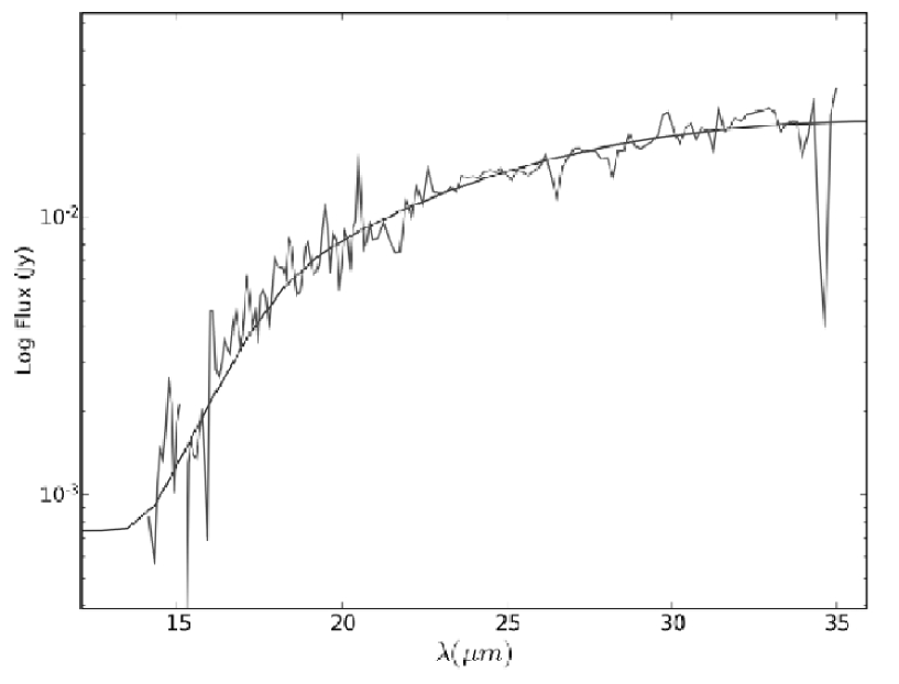
Figure 2.1: Background-subtracted Spitzer IRS spectrum of warm dust in SNR 0509-67.5, with model overlaid. The model will be discussed further in chapter 7. Note absence of lines in the spectrum.

IR emission from SNRs is predominantly thermal emission from warm dust grains, heated via collisions with hot electrons and ions in the post-shock gas. Although IR line emission can become strong once a shock reaches its radiative phase, it is virtually non-existent in fast, non-radiative shocks, as Figure 2.1 shows. This work focuses on emission from these non-radiative shocks, which typically persist for hundreds or thousands of years in SNRs before becoming radiative.

2.1 What is Dust?

Dust grains in the ISM are not like the dust that accumulates on top of TVs and countertops. ISM grains are microscopic, ranging in size from molecules of a few atoms to small solid bodies, several microns ($\mu$m, where 1 $\mu$m = 10^-6 meters) in radius. Grains are made up of various elements, most notably carbon (which can exist in either crystalline forms like graphite or in amorphous forms), oxygen, silicon, magnesium, and iron. Polycyclic aromatic hydrocarbons (PAHs) have also been spectroscopically identified as residing in the ISM. These molecules are similar to PAHs produced on Earth, typically as byproducts of fuel burning. PAHs consist of aromatic rings of carbon with hydrogen atoms at their edges. On average, about 0.1-1% of the mass of the ISM is contained in dust grains, with the remainder being in the gaseous phase.

2.2 Dust Formation Sites

Dust plays an important role in both the evolution the ISM in galaxies and the universe as a whole. It plays an important role in star formation, acting as a catalyst for the formation of H₂ molecules, which are efficient coolants, giving dense clouds a chance to contract and create new stars. Early observations of the disk of the Milky Way galaxy showed dark lanes of dust that block starlight, and high-redshift observations of galaxies in the early universe show large quantities of dust present shortly after the Big Bang.

Dust condensation requires an abundance of heavy elements, a dense environment where collisions between particles are frequent, and a low temperature below the vaporization temperature for grains. These conditions are not frequently found together in the universe, but two sites are often suggested as potential hosts for dust nucleation: atmospheres of AGB stars and supernovae. AGB stars are beyond the scope of this work, but the amount of dust produced in supernovae can be determined from observations of SNRs, and will be discussed at length in a later chapter. Theoretical calculations of the amount of dust produced in the ejecta of CC SNe can exceed several solar masses (Nozawa et al. 2007). However, more recent work by Cherchneff & Dwek (2010) has revised these estimates down by about a factor of 5.

2.3 Observing Dust Emission

The majority of heating of grains in the ISM is done via radiative heating by photons. This heating can be from stars, active galactic nuclei, or the interstellar radiation field. For this work, however, I focus on collisional heating by particles behind shock waves. Collisionally heated grains in SNRs are typically warmed to temperatures of 50-200 K, which is far too cold to be observed by optical, ground-based instruments. Grains at this temperature radiate in the mid-IR, with their spectra peaking anywhere from 20-100 $\mu$m. To effectively observe at these wavelengths, one needs to travel outside the Earth’s atmosphere, above the water vapor that significantly absorbs mid and far-IR radiation. The majority of the work described here is based on observations done by the Spitzer Space Telescope.

2.3.1 Spitzer

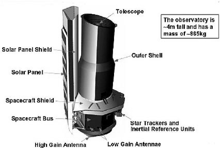
Figure 2.2: Diagram of the Spitzer Space Telescope, taken from http://www.nasa.gov/missions/deepspace/f_spitzerbirth_prt.htm

NASA’s Spitzer Space Telescope is the fourth and final mission in the “Great Observatories” program, following the Hubble Space Telescope (1990-present, optical wavelengths), the Compton Gamma-Ray Observatory (1991-2000, gamma-rays), and the Chandra X-ray Observatory (1999-present, X-rays). All four instruments were large space-based observatories. Spitzer was launched in August of 2003 and began full-time science operations in 2004. Unlike the other observatories in the program, with orbits around the Earth, Spitzer follows a heliocentric orbit that recedes away from Earth at the rate of 0.1 astronomical units (AU) per year. Both the Earth and the Moon are incredibly bright IR sources, and the telescope had to be placed far away from both to achieve its desired sensitivity. The spacecraft (see Figure 2.2) consists of an 85-centimeter telescope outfitted with 3 separate instruments which can be placed in the field of view at any given time. A sun-shield, which always faces the Sun, protects the entire system, acting as the first line of defense against photons that would warm the telescope and damage the instruments. The telescope is cryogenically cooled, with the primary coolant being liquid helium. This keeps the detectors at 4.2 K, necessary for science observations in the mid and far-IR, but comes at a price: the liquid helium is an expendable resource and cannot last forever. The target lifetime for the “cold mission” (i.e., time before the cryogen ran out) of Spitzer was 5 years; in reality, it lasted over 5.5 years before running out in May of 2009. Thus began the “warm mission” of Spitzer, involving only the shortest IR wavelengths, which is expected to last until 2013.

2.3.2 Spitzer’s Instruments

Spitzer has three instruments onboard, data from all of which is featured in this work. The Infrared Array Camera (IRAC) provides photometric (imaging) capabilities in the near and mid-IR, with four channels covering the wavelength range of 3.3-8.5 $\mu$m. The Multi-band Imaging Photometer for Spitzer (MIPS) contains three broadband channels for photometric imaging, centered at 24, 70 and 160 $\mu$m for channels 1, 2, and 3, respectively. Spectroscopically, the Infrared Spectrograph (IRS) provides both low and medium spectral resolution data over the wavelength range of 5-40 $\mu$m. The low-resolution spectrograph uses slit spectroscopy and is ideal for continuum detection; its resolution, $\lambda/\delta\lambda$, is 64-128. The high-resolution module uses echelle spectrographs ideal for observing lines, provides a resolution of $\lambda/\delta\lambda$ = 600. Both IRAC and MIPS provide diffraction limited optics, with the angular resolution ranging from $\sim 1^{\prime\prime}$ for the 3.6 $\mu$m array to $\sim 50^{\prime\prime}$ at 160 $\mu$m.

2.4 Size Distribution of ISM Dust Grains

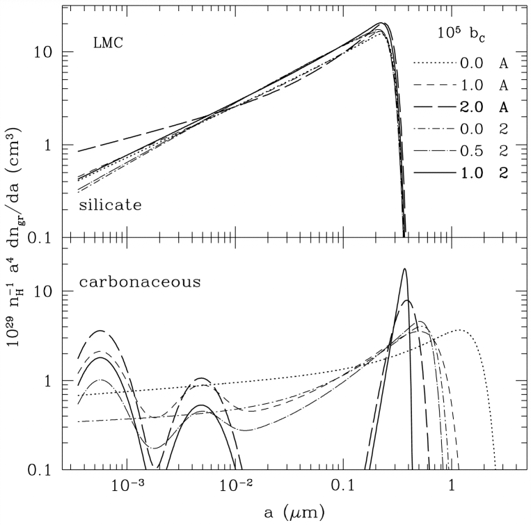
Figure 2.3: Figure 18 from Weingartner and Draine (2001), showing the size distribution of silicate (top) and carbonaceous grains (bottom) for the Large Magellanic Cloud. For this work, we use their model “2.0 A.”

Since dust can exist in all varieties and sizes, it is necessary to have a more quantitative understanding of the distribution of these various grains in the ISM. Numerous authors (Mathis et al. 1977, Weingartner & Draine 2001, hereinafter WD01, Zubko et al. 2004 and more) have attempted to quantify the size distribution for both the galaxy and the Magellanic Clouds (dwarf satellite galaxies of the Milky Way). This work primarily uses the distributions of WD01, shown in Figure 2.3, although alternative models are explored. As can be seen in the figure, the size distribution of grains is steeply weighted towards the small end. This is not unexpected, since it is believed that grains coalesce in dense environments and grow in size. Shattering of grains in grain-grain collisions may also play a major role in establishing the ISM grain size distribution.

2.5 Grain Heating and Cooling

Dust grains in the ambient ISM are heated by the interstellar radiation field, primarily by UV starlight. This radiation field can heat dust to $\sim 10-20$ K, and warmer dust is often found in the immediate vicinity of stars. In SNRs, however, the primary heating mechanism for grains is collisional heating, where grains are warmed by frequent collisions with the hot ($>10^{6}$ K) electrons and ions in the post-shock region behind the forward shock. The heating rate for a grain immersed in a hot plasma is given by

$$H=\left(\frac{32}{\pi m}\right)^{1/2}\pi a^{2}n(kT)^{3/2}h(a,T),$$ (17)

where $m$ is the mass of the impinging particle (proton, electron, etc.), $a$ is the radius of the grain, $n$ is the density of the gas, $k$ is Boltzmann’s constant, $T$ is the temperature of the gas, and $h(a,T)$ is a function that describes the efficiency of the energy deposition rate of a particle at a given $T$ for a grain with radius $a$. It can be immediately seen from this equation that at a fixed $T$, electrons will dominate the heating over protons, since their mass is much smaller and they move much faster.

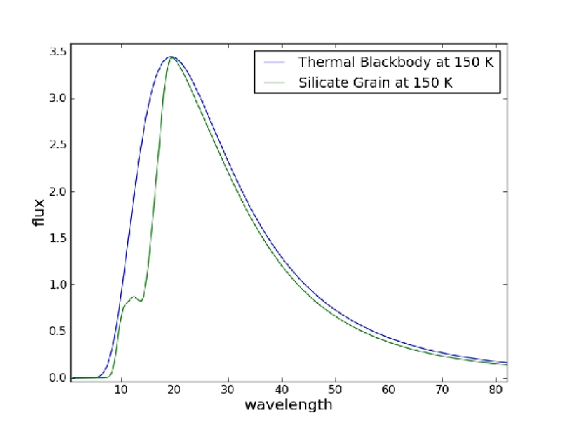
Figure 2.4: Comparison of thermal blackbody at 150 K (blue) with single silicate grain at 150 K (green).

Since grains are virtually always smaller than the wavelength of light they emit (i.e. $a<<\lambda$), they will cool as modified blackbodies (see Figure 2.4). The cooling rate of a given grain at a temperature $T_{d}$ is given by

$${\cal L}=\int^{\infty}_{0}d\nu C_{abs}(\nu)4\pi B_{\nu}(T_{d}),$$ (18)

where $\nu$ is the frequency, $C_{abs}$ is the absorption cross section, and $B_{\nu}(T)$ is the Planck blackbody function. Calculating the quantity $C_{abs}$ requires knowledge of the dielectric function, $\epsilon$, of a given grain material. For an excellent review, see Draine (2004). In equation (32) of that paper, the absorption cross section for a sphere is given by (assuming $a<<\lambda$)

$$C_{abs}=\frac{9\nu V}{c}\frac{\epsilon_{2}}{(\epsilon_{1}+2)^{2}+\epsilon_{2}^{2}},$$ (19)

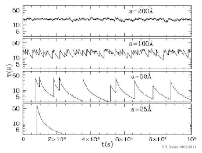
Figure 2.5: Figure 17 from Draine (2003), showing grain temperature vs. time for 4 different grain sizes, heated by photons from the interstellar radiation field. A similar stochastic heating process occurs for collisionally heated grains.

where $c$ is the speed of light, $V$ is the grain volume, $\epsilon_{1}$ is the real part of $\epsilon$, and $\epsilon_{2}$ is the imaginary part. It is readily seen that in the limit of $a<<\lambda$, $C_{abs}$ is proportional to grain volume. This is in contrast to the heating rate, where heating was proportional to the surface area of the grain. As a result, the equilibrium temperature for a grain immersed in a plasma is a function of its size, even if all other grain properties are identical. Additionally, small grains (i.e. grains that have a sufficiently large surface-to-volume ratio) may find collisions so infrequent and cooling times so rapid that they never reach an equilibrium temperature, and instead constantly fluctuate, spiking to high temperatures and emitting radiation much more efficiently when at their maximum temperatures. See Figure 2.5 for plots of grain temperature versus time.

2.6 Dust Grain Sputtering

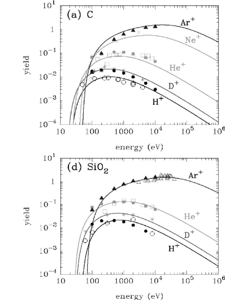
Figure 2.6: Figure 1a and 1d of Nozawa et al. (2006), showing the sputtering yield as a function of impinging particle energy for a variety of ions into carbonaceous and SiO₂ grains.

The same collisions that heat grains can also slowly destroy them via sputtering. Sputtering is the ejection of atoms from the surface of a grain during collisions with ions. This loss of material reduces the size of the grain, and the ejected atoms are liberated back into the gaseous phase. Thus, as a function of time, large grains are converted into small grains, and small grains are completely destroyed in the post-shock region of a SNR. This strongly modifies the grain size distribution behind the shock. Nozawa et al. (2006) provides the sputtering yield (number of particles ejected per collision) as a function of impinging particle energy for various particles and dust compositions (see Figure 2.6).

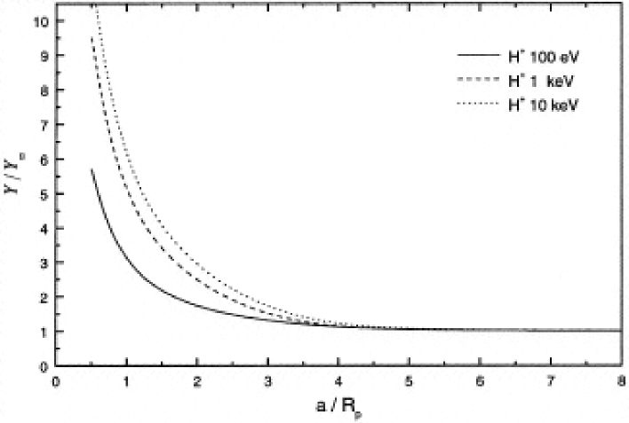
Figure 2.7: Figure 3a from Jurac et al. (1998), showing the enhancement in yield for protons of various energies, scaled to the yield for isotropic bombardment of a flat surface (semi-infinite solid approximation).

The equations given in Nozawa et al. are taken from Bodhansky (1984), which calculates sputtering of solids with respect to industrial applications, particularly that of building a nuclear reactor. For these applications, the bulk approximation of a solid is acceptable, as one never has to worry about the sides and back walls of the reactor. For sufficiently small grains, however, these equations are not sufficient, because sputtering can take place not only from the front side of the grain where the initial impact occurs, but also from the sides and back. Specifically, Jurac et al. (1998) find that for grains with $a$ $<$ 3R_P, where R_P is the projected range of a particle impacting a grain (where projected range is the average of the depth to which a particle will penetrate the grain in the course of slowing down), the sputtering yields are enhanced. For the smallest of grains, this can lead to an order-of-magnitude increase in the sputtering rate, as shown in Figure 2.7.

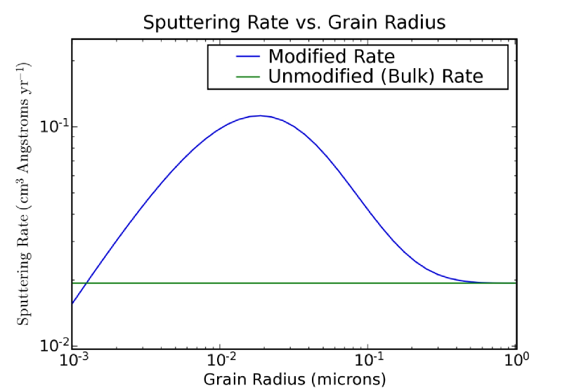
Figure 2.8: Sputtering rate as a function of grain radius, where sputtering is done by protons with energy 10 keV. Rates used in code shown in blue, bulk solid approximation shown in green. Increase in rate from $10^{-2}-10^{-1}$ $\mu$m due to enhancement of sputtering for small grains, dropoff short of $\sim 10^{-2}$ $\mu$m due to decreased energy deposition rate for energetic particles.

Finally, there is a competing effect for small grains. Sufficiently fast impinging protons do not deposit all of their energy into a grain when they collide; the rate at which they deposit energy is a function both of the grain radius and the energy of the particle. As small grains become transparent to protons, protons deposit less energy in collisions with nuclei within grains, so sputtering rates are reduced relative to Jurac et al. results (Serra Dìaz-Cano & Jones, 2008). We therefore scale sputtering yields for small grains in proportion to the fractional energy deposited by the proton or alpha particle. Figure 2.8 shows the sputtering yield as a function of grain radius for a 10 keV proton.

2.7 Modeling Grain Emission in SNR Shocks

In order to create a model for collisionally heated dust emission in the post-shock gas of an SNR, everything outlined above must be taken into account. One must have an underlying model for the grain physics, including the grain size distribution for each species of grain. In this work, unless stated otherwise, we model dust in the ISM as consisting of “astronomical silicate” (with predominantly MgFeSiO₄ composition) (Draine & Lee 1984) and graphite grains, mixed in the proportions given in WD01. Optical constants ($\epsilon_{1}$ and $\epsilon_{2}$) are taken from Draine & Lee (1984), and sputtering yields are calculated as described above. We use 100 grain sizes, logarithmically spaced from 1 nm to 1 $\mu$m. Although smaller grains are thought to be present in the ISM, we assume that they are instantaneously destroyed in the shock and contribute nothing to the emission seen by Spitzer (Micelotta et al., 2010). Given Spitzer’s limited spatial resolution and the small number of remnants that are large enough to resolve the immediate post-shock region, this is likely a good approximation.

The energy deposition rates of electrons and protons as a function of energy and grain size must also be input to the code, as well as the optical constants of various grain types. Since the heating rate of grains depends on the density and temperature of different particle species within the plasma, these must be included in the code. The total sputtered number of atoms for a given grain depends on the time it has been immersed in the plasma, i.e., the time since it was shocked. This can be quantified by a parameter known as the “sputtering timescale”, defined as $\tau=\int^{t}_{0}n_{p}dt$, where $n_{p}$ is the post-shock proton density. This is similar to the “ionization timescale” found in X-ray analysis, defined as $\tau_{i}=\int^{t}_{0}n_{e}dt$, where $n_{e}$ is electron density. In order to model a region of any significant spatial width behind the shock, it is necessary to create a shock model which superimposes regions of different $\tau$ behind the shock. In the models described in this paper, this is done by calculating the sputtering rate for all grains in the distribution in each zone behind the shock, and adjusting the grain size distribution accordingly. The final model appropriately sums these post-shock distributions.

The output of such a model is the temperature of each grain in the distribution, which is size-dependent. To account for stochastic heating effects on small grains, we use a method devised by Guhathakurta & Draine (1989). Since the sputtering rates for grains are calculated in the shock model, we can integrate them to obtain the total amount of mass in grains that is destroyed. Of course, this mass is not actually destroyed, merely converted back into the gaseous phase. The thermal spectrum for each grain is calculated and summed over the final distribution to create a single spectrum, which can be compared directly to observations.

2.8 Necessity for a Multi-Wavelength Approach

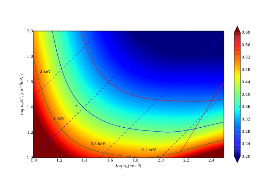
Figure 2.9: The 70/24 $\mu$m MIPS flux ratio for Kepler’s SNR (see Chapter 6) as a function of electron density, $n_{e}$ and pressure, $n_{e}kT_{e}$. The background color scale indicates 70/24 $\mu$m ratio, as indicated by the color bar at right. Dashed lines are lines of constant temperature. The solid magenta diagonal line at lower right indicates where the modeled shocks would become radiative, assuming solar abundance models and an age of 400 yr. Three solid curves are lines of constant 70/24 $\mu$m MIPS flux ratios, 0.30, 0.40, and 0.52 (from top to bottom). Position of a Balmer-dominated fast shock is marked by a star. There are many combinations of density and temperature that can yield an identical 70/24 $\mu$m flux ratio.

In theory, one can tune any or all of the parameters in the model to fit the observed data from Spitzer or other telescopes. In practice, however, there are significant degeneracies present in the model. Figure 2.9 shows an example of these degeneracies for only two components, electron density and temperature. It is impossible, from IR data alone, to eliminate the degeneracies; so we must use information from other wavelengths as additional constraints on the modeling.

2.8.1 X-rays

Thermal X-ray spectra are most sensitive to the electron temperature of the shocked gas. Since both the shocked ambient medium and the reverse-shocked ejecta are strong X-ray emitters, it is necessary to separate (either spatially or spectroscopically) the components belonging to each to get an accurate measure of the temperature in the post-shock gas. As discussed in Chapters 3-5, we see very little evidence for dust emission from ejecta in most SNRs, and thus are typically only concerned about dust heated by the forward shock. A shock model of an X-ray spectrum can also give the ionization timescale. If the SNR is large enough and/or young enough, high spatial resolution instruments like Chandra may be able to resolve proper motion of the forward shock itself, yielding a shock velocity. This is subject to uncertainties about the distance to the object, which is often not well known.

2.8.2 Optical/UV

Optical emission from non-radiative shocks shows line emission from both stationary atoms in the post-shock gas and fast-moving hydrogen atoms, created by thermal protons, that have undergone charge-exchange (i.e. the stealing of an electron) with slow neutrals entering the shock. This requires at least partially-neutral material ahead of the shock, and creates a fast-moving neutral atom moving with bulk velocity $(3/4)v_{s}$ (for standard shock jump conditions), where $v_{s}$ is the shock speed. The fast-moving neutrals are collisionally excited by free electrons and protons, emitting radiation primarily via the $n=3\rightarrow 2$ (Balmer-$\alpha$, or H$\alpha$ 656.3 nm optical line) and the $n=2\rightarrow 1$ (Lyman-$\alpha$, 121.6 nm ultraviolet line) transitions. This produces a “broad” hydrogen line, where the broadening is a result of two (additive) phenomena: thermal line broadening resulting from the random motions of the hot neutrals in the shock frame, and Doppler broadening resulting from the bulk velocities of the post-shock gas seen along a line-of-sight through the front and back sides of the SNR. Hydrogen lines measured directly on the limbs of the remnant show only thermal broadening, while lines measured at any point interior to the outer shell show additional broadening from the Doppler component. This broad line can be used as a diagnostic of shock speed and proton temperature in the post-shock gas.

A narrow component is also seen in optical/UV spectra of SNRs, arising from collisional excitation of cold neutral atoms that survive passage of the shock. The intensity ratio of the broad and neutral components is sensitive to both the shock speed and the degree of equilibration between electrons and protons at the shock front (Chevalier 1980). Excitations of H in collisions with protons and alpha particles are most important at high shock speeds; electrons dominate at low shock speeds. High spatial resolution optical images can also be used to measure the proper motion of some SNR shocks.

2.9 Density Diagnostics

The density of the gas, either pre-shock or post-shock, is difficult to determine from either X-ray or optical observations. X-rays can give a measure of the root mean square (r.m.s.) post-shock density through the emission measure, defined as $EM=\int^{V}_{0}dVfn_{e}n_{H}$, where $n_{e}$ and $n_{H}$ are the post-shock electron and proton densities, respectively, but this is dependent on $f$, the filling fraction of the material in the volume considered. H$\alpha$ line strength measurements can yield the total number of hydrogen atoms entering the shock at a given time, but only if the pre-shock neutral fraction is known a priori. IR modeling of warm dust emission provides an independent diagnostic that does not depend on these uncertainties. If one knows the gas temperature and energy deposition function, the heating of a grain is dependent only on the grain size and gas density. Matching model results to observed IR spectra, with density as a tunable parameter, gives a fit to the post-shock density.

Although IR modeling is not sensitive to pre-shock density, it is nonetheless possible to use inferences derived from IR and X-ray fits to constrain this quantity. X-ray spectral fitting provides the EM of the gas, as defined above. This quantity can be rewritten (if $n_{e}$ is constant) as $EM\propto n_{e}M_{g}$, where $M_{g}$ is the mass in gas that has been swept-up by the forward shock, defined by $M_{g}\propto\int^{V}_{0}dVfn_{H}$. If the post-shock electron density can be independently determined, as is the case in modeling IR spectra, then this quantity can be divided out of the EM, leaving the quantity of gas shocked by the remnant. This method is independent of the filling fraction of the gas, since it merely measures the total amount of swept-up gas, regardless of its distribution. If the distance to the remnant is well known, this total amount of gas can be divided by the volume enclosed by the forward shock to obtain the average pre-shock density in the ambient ISM. The implicit assumption in this method is that $\rho_{ISM}$ is constant.

2.9.1 Errors on Density

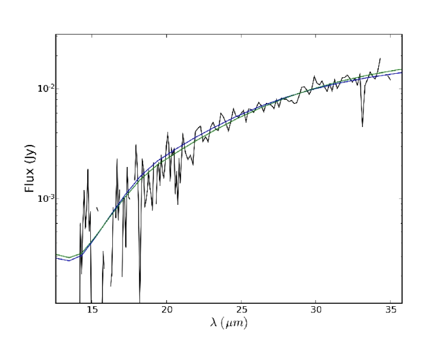
Figure 2.10: Spitzer IRS data of “faint” region (see Chapter 8) of 0509-67.5, overlaid with 90% confidence limits from model fit. The best-fit density for this data was $n_{p}$ = 0.88 cm^-3 (not shown), and the 90% confidence lower and upper limits are 0.7 and 1.0 cm^-3, shown in green and blue, respectively. $\chi^{2}$ fits were only performed in the region from 21-32 $\mu$m, where signal-to-noise was strongest.

The shape of a dust spectrum is a fairly sensitive function of the gas density. Although errors on derived quantities are model dependent, at the very least one can make an estimate of the validity of results reported in the following chapters from a purely statistical point of view. Figure 2.10 shows a spectrum from a region of SNR 0509-67.5 (discussed at length in Chapter 8), overlaid with two models. These models represent the 90% confidence limits on the fits using $\chi^{2}$ statistics, varying only the post-shock density. For a given model fit to a dataset, $\chi^{2}$ is given by

$$\sum_{i=1}^{n}(\frac{X_{i}-\mu_{i}}{\sigma})^{2},$$ (20)

where $X_{i}$ is the value of the $i$th data point, $\mu_{i}$ the value of the $i$th model point, and $\sigma$ the standard deviation of the dataset. Once a best fit value for a given parameter is found by minimizing the value of $\chi^{2}$, the 90% confidence limits are found by varying the parameter until $\delta\chi^{2}$ = 2.71. The best fit was obtained with a density of $n_{p}$ = 0.88 cm^-3, and the 90% error limits are 0.7 and 1.0 cm^-3. Thus, one can expect errors of order 20% in densities derived in IR fits, within the framework of a given model.

2.9.2 Application to Particle Acceleration in Shocks

This multi-wavelength approach to determining both the pre- and post-shock densities provides more robust estimates than analysis in either wavelength could alone. Knowing both densities allows a direct measurement of the compression ratio of the forward shock, defined as $\rho_{2}/\rho_{1}$. Using the standard shock jump conditions found in Chapter 1, this ratio for a strong shock should be 4. If, however, cosmic rays are being accelerated in SNRs, the energy deposited into these particles would have to come from somewhere. An alternative sink for shock thermal energy is the turbulent magnetic fields found in the immediate vicinity of the shock. Specifically, diffusive shock acceleration (Bell 1978, Jones & Ellison 1991), a process by which the particles scatter back and forth across the shock off from magnetic field irregularities, thus gaining a substantial amount of energy, is widely believed to be the process which robs the shock of energy. This process is believed to be capable of accelerating particles up to the knee of the cosmic-ray spectrum, which occurs at roughly $10^{15}$ eV. In fact, if supernova shocks are the sole source of cosmic rays in the galaxy, accounting for the cosmic-ray energy density observed requires that $\sim 10$% of the kinetic energy of a supernova explosion ($\sim 10^{51}$ ergs) must be transferred to cosmic rays.

If such a process is happening, as appears the case with at least some young SNRs (Abdo et al. 2010), the shock jump conditions found in chapter 1, which ignore the contributions of cosmic rays or magnetic fields, would no longer be strictly valid. The robbing of energy from the post-shock gas to be injected into cosmic rays would increase the magnetic field amplification at the shock, lower the temperature of the post-shock gas, and increase the compression ratio of the gas. Efforts have been made to measure the magnetic field amplification (Uchiyama et al. 2007) and the correlation between shock speed and post-shock gas temperature (Helder et al. 2009), but observational confirmation of the increased compression ratio at the forward shock is difficult to obtain. The method detailed above could provide measurements, or at the very least, constraints, on this number.

3 Dust Destruction in Type Ia Supernova Remnants in the Large Magellanic Cloud

This chapter is reproduced in its entirety from Borkowski, K.J., Williams, B.J., Reynolds, S.P., Blair, W.P., Ghavamian, P., Sankrit, R., Hendrick, S.P., Long, K.S., Raymond, J.C., Smith, R.C., Points, S., & Winkler, P.F. 2006, ApJ, 642, 141.

3.1 Introduction

The dust content in galaxies, dust composition, and grain size distribution are determined by the balance between dust formation, modification in the interstellar medium (ISM), and destruction (Draine, 2003). Some evidence exists for dust formation in the ejecta of core-collapse supeyrnovae (e.g., SN 1987A; de Kool, Li, & McCray, 1998) but no reports exist for SNe Ia. Dust destruction is intrinsically linked to SN activity, through sputtering in gas heated by energetic blast waves and through betatron acceleration in radiative shocks (Jones, 2004). Dust destruction in SNRs can be studied by its strong influence on thermal IR emission from collisionally heated dust. The IRAS All Sky Survey provided fundamental data on Galactic SNRs (Arendt, 1989; Saken et al., 1992). This prompted extensive theoretical work on dust heating, emission, and destruction within hot plasmas, summarized by Dwek & Arendt (1992). Theory is broadly consistent with IRAS observations, but limitations of those observations (low spatial and spectral resolution and confusion with the Galactic IR background) precluded any detailed comparisons. In particular, while it is clear that thermal dust emission is prevalent in SNRs, our understanding of dust destruction is quite poor.

To examine the nature of dust heating and destruction in the interstellar medium, we conducted an imaging survey with the Spitzer Space Telescope (SST) of 39 SNRs in the Magellanic Clouds (MCs). We have selected a subset of our detections, four remnants of Type Ia supernovae, to address questions of dust formation in Type Ia ejecta, dust content of the diffuse ISM of the LMC, and dust destruction in SNR shocks. Both DEM L71 (0505-67.9; Rakowski, Ghavamian, & Hughes 2003) and 0548–70.4 (Hendrick, Borkowski, & Reynolds 2003) show X-ray evidence for iron-rich ejecta in the interior, and both have well-studied Balmer emission from nonradiative shocks (Ghavamian et al., 2003; Smith et al., 1991). Two smaller remnants, 0509–67.5 and 0519–69.0, also show prominent H$\alpha$ and Ly$\beta$ emission from nonradiative shocks (Tuohy et al. 1982; Smith et al. 1991; Ghavamian et al. 2006, in preparation). There appears to be little or no optical contribution from radiative shocks. Confusion in IR is widespread in the LMC, but our remnants are less confused than typical, easing the task of separating SNR emission from background.

3.2 Observations and Data Reduction

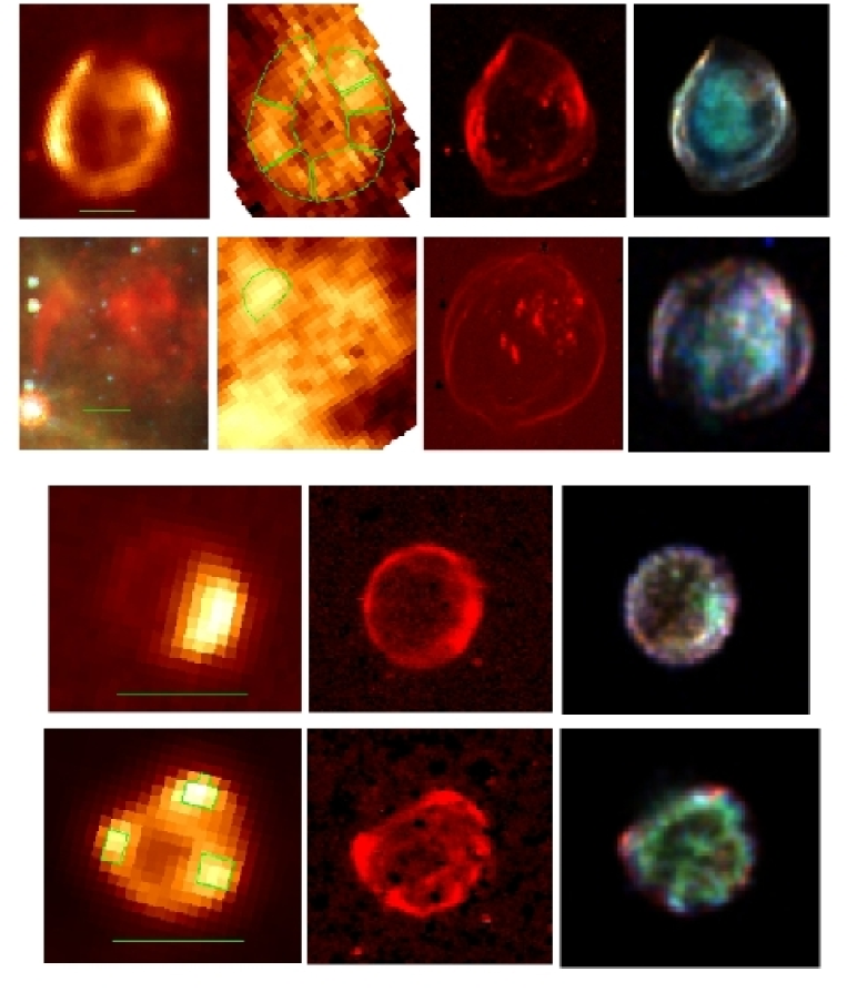
Figure 3.1: Top row: DEM L71 at 24 and 70 $\mu$m, H$\alpha$, and X-ray (red, 0.3 – 0.7 keV; green, 0.7 – 1.0 keV; blue, 1.0 – 3.5 keV; smoothed with 1 pixel Gaussian). Second row: 0548–70.4 with red, 24 $\mu$m; green, IRAC 8.0 $\mu$m; blue $\mu$m, IRAC 5.8 $\mu$m; 70 $\mu$m; H$\alpha$, and X-ray image as for DEM L71, smoothed with a 2 pixel Gaussian. Third row: 0509–67.5 at 24 $\mu$, H $\alpha$, and X-ray: red, 0.3 – 0.7 keV; green, 0.7 – 1.1 keV and blue, 1.1 – 7.0 keV, Bottom row: 0519–69.0, as in third row. Half-arcminute scales are shown for each SNR.

We observed all four objects in all four bands of the Infrared Array Camera (IRAC), as well as with the Multiband Imaging Photometer for Spitzer (MIPS) at 24 and 70 $\mu$m. Each IRAC observation totaled 300 s (10 30-s frames); at 24 $\mu$m, 433 s total (14 frames); and at 70 $\mu$m, 986 s total (94 frames) for all but 0548–70.4, for which we observed a total of 546 s in 52 frames. The observations took place between November 2004 and April 2005. Images are shown in Figure 3.1. Confusion from widely distributed warm dust made many 70 $\mu$m observations problematic, but we obtained useful data on both DEM L71 and 0548–70.4.

MIPS images were processed from Basic Calibrated Data (BCD) to Post-BCD (PBCD) by v. 11 of the SSC PBCD pipeline. For the 24 $\mu$m images, we then re-mosaicked the stack of BCD images into a PBCD mosaic using the SSC-provided software MOPEX, specifically the overlap correction, to rid the images of artifacts. For the 70 $\mu$m data, we used the contributed software package GeRT, provided also by the SSC, to remove some vertical streaking. IRAC images were also reprocessed using MOPEX to rid the image of artifacts caused by bright stars.

All four remnants were clearly detected at 24 $\mu$m, with fluxes from indicated regions reported in Table 3.1. As Figure 1 shows, emission is clearly associated with the X-ray-delineated blast wave, though not with interior X-ray emission. Since we expect line emission from fine-structure transitions of low-ionization material to be a significant contributor only in cooler, denser regions identified by radiative shocks, we conclude that the emission we detect is predominantly from heated dust. None of our objects was clearly detected at 8 $\mu$m, with fairly stringent upper limits shown in Table 3.1.

3.3 Discussion

We modeled the observed emission assuming collisionally heated dust (e.g., Dwek & Arendt, 1992). The models allow an arbitrary grain-size distribution, and require as input parameters the hot gas density $n$, electron temperature $T_{e}$, ion temperature $T_{i}$, and shock sputtering age $\tau=\int_{0}^{t}n_{p}dt$. The models use an improved version of the code described by Borkowski et al. (1994), including a method devised by Guhathakurta & Draine (1989) to account for transiently-heated grains, whose temperature fluctuates with time and therefore radiate far more efficiently. The energy deposition rates by electrons and protons were calculated according to Dwek (1987) and Dwek & Smith (1996). We used dust emissivities based on bulk optical constants of Draine & Lee (1984). Our non-detections in IRAC bands showed that small grains are destroyed, so it was not necessary to model emission features from small polycyclic aromatic hydrocarbon (PAH) grains. The preshock grain size distribution was taken from the “provisional” dust model of Weingartner & Draine (2001), consisting of separate carbonaceous and silicate grain populations, in particular their average LMC model with maximal amount of small carbonaceous grains. Sputtering rates are based on sputtering cross sections of Bianchi & Ferrara (2005), augmented by calculations of an enhancement in sputtering yields for small grains by Jurac et al. (1998). We have modeled 1-D shocks, that is, superposed emission from regions of varying sputtering age from zero up to a specified shock age (Dwek, Foster, & Vancura, 1996).

To estimate shock parameters, we used the non-radiative shock models of Ghavamian et al. (2001) to model the broad component H$\alpha$ widths and broad-to-narrow H$\alpha$ flux ratios measured by Tuohy et al. (1982) and Smith et al. (1991) for the LMC SNRs. Results for electron and proton temperatures $T_{e}$ and $T_{p}$ are quoted in Table 3.2. For 0509–67.5, we assumed $T_{e}/T_{p}\leq 0.1$ at the shock front, consistent with the observed Ly$\beta$ FWHM of 3700 km s^-1 (Ghavamian et al. 2006, in preparation). For Sedov dynamics, the sputtering age $\tau$ (which is also the ionization timescale) reaches a maximum of about $(1/3)n_{p}t$ where $t$ is the true age of the blast wave (Borkowski, et al., 2001). Therefore we use an “effective sputtering age” of $n_{p}t/3$ when calculating effects of sputtering.

3.3.1 DEM L71 and 0548–70.4

These two remnants have been well-studied in X-rays (DEM L71: Rakowski et al. 2003; 0548–70.4, Hendrick et al. 2003). They have ages of 4400 and 7100 yr, respectively, derived from Sedov models. For DEM L71, Ghavamian et al. (2003) were able to infer shock velocities over much of the periphery, ranging from 430 to 960 km s^-1, consistent with X-ray inferences (Rakowski et al., 2003).

To model DEM L71, we used parameters deduced from Chandra observations (Rakowski et al., 2003), averaged over the entire blast wave since different subregions were fairly similar. We find a predicted 70/24 ratio in the absence of sputtering ($\tau=0$) of about 2.3 (including only grains larger than 0.001 $\mu$m in radius), compared to the observed 5.1. Using an effective age of 1/3 the Sedov age gave a value of 5.1. Table 3.3 also gives the total dust mass we derive, and the total IR luminosity produced by the model.

For 0548–70.4, both the east and west limbs and some bright knots of interior emission are visible at 24 $\mu$m, but only the north half of the east limb is clearly detected at 70 $\mu$m. Only fluxes from this region were measured; the results are summarized in Table 3.1. Using a 1-D model for Coulomb heating of electrons by protons, we calculate a mean electron temperature in the shock region of $T_{e}\sim 0.66$ keV. A model using the postshock density of 0.72 cm^-3 obtained by Hendrick et al. (2003) for the whole limb (including sputtering) gives too high a 70/24 $\mu$m ratio. That ratio is very sensitive to density; we found that increasing $n_{p}$ by a factor $<2.5$ adequately reproduced the observed ratio. That fitted density appears in Table 3.2 and the corresponding results are in Table 3.3. Gas mass was derived from the X-ray emission measure of the east limb (Hendrick et al., 2003), scaled to the region shown in Figure 1, and using electron density in Table 3.2.

3.3.2 0509–67.5 and 0519–69.0

Our other two objects are much smaller; X-ray data suggest young ages (Warren & Hughes, 2004). Detections of light echoes (Rest et al., 2005) indicate an age of about 400 yr for 0509–67.5 and about 600 yr for 0519–69.0, with $\sim 30$% errors. Much higher shock velocities inferred by Ghavamian et al. (2006, in preparation) mean that plasma heating should be much more effective. Higher dust temperatures, hence lower 70/24 $\mu$m ratios, should result. In fact, we did not detect either remnant at 70 $\mu$m, with upper limits on the ratio considerably lower than the other two detections (Table 3.1).

In the case of 0509-67.5, optical-UV observations fix only $T_{p}$, so we regarded the density $n_{p}$ as a free parameter, fixing $\tau$ at $n_{p}t/3$ and finding $T_{e}$ assuming no collisionless heating. Our 70 $\mu$m upper limit gives a lower limit on $n_{p}$, shown in Table 3.2, as well as an upper limit on the total dust mass (Table 3.3).

The analysis of 0519-69.0 was identical to that done for 0509-67.5. However, for 0519-69.0 we divided the remnant up into two regions: the three bright knots (which we added together and considered one region, accounting for 20% of the total flux) and the rest of the blast wave. Optical spectroscopy (Ghavamian et al. 2006) allowed determination of parameters separately for the knots and the remainder. Again regarding $n_{p}$, $T_{e}$ and $\tau$ as free parameters, we place lower limits on the post-shock densities and $T_{e}$, and upper limits on the amount of dust mass, including sputtering. For both remnants, density limits assume the effective sputtering age; if there is no sputtering at all, we obtain firm lower limits on density lower by less than a factor of 2.

3.4 Results and Conclusions

The IR emission in the Balmer-dominated SNRs in the LMC is spatially coincident with the blast wave. It is produced within the shocked ISM by the swept-up LMC dust heated in collisions with thermal electrons and protons. We find no evidence for infrared emission associated with either shocked or unshocked ejecta of these thermonuclear SNRs. While detailed modeling of small grains is required to make a quantitative statement, apparently little or no dust forms in such explosions, and any line emission produced by ejecta is below our detection limit. This is consistent with observations of Type Ia SNe where dust formation has never been observed. It is also consistent with the absence in meteorites of presolar grains formed in Type Ia explosions (Clayton & Nittler, 2004).

The measured 70/24 $\mu$m MIPS ratios in DEM L71 and 0548-70.4, and the absence of detectable emission in the IRAC bands in all 4 SNRs, can be accounted for with dust models which include destruction of small grains. Without dust destruction, numerous small grains present in the LMC ISM (e.g., Weingartner & Draine, 2001) would produce too much emission at short wavelengths when transiently heated to high temperatures by energetic particles. Destruction of small grains is required to reproduce the observed 70/24 $\mu$m MIPS ratios in DEM L71 and 0548-70.4: 90% of the mass in grains smaller than 0.03–0.04 $\mu$m is destroyed in our models. Even with this destruction, we infer pre-sputtering dust/gas mass far smaller than the 0.25% in the Weingartner & Draine model.

The two young remnants, 0509–67.5 and 0519–69.0, have been detected only at 24 $\mu$m, but our rather stringent upper limits at 70 $\mu$m suggest the presence of much hotter dust than in the older SNRs DEM L71 and 0548-70.4. Such hot dust is produced in our plane shock models only if the postshock electron densities exceed $1.6$ cm^-3 and 3.4–7.7 cm^-3 in 0509–67.5 and 0519–69.0, respectively (Table 3.2). 0509–67.5 is asymmetric, and the quoted lower density limit needs to be reduced if an average postshock electron density representative of the whole SNR is of interest. We measure a flux ratio of 5 between the bright and faint hemispheres, depending primarily on the gas density ratio between the hemispheres, and on the ratio of swept-up ISM masses. For equal swept-up masses, our models reproduce the observed ratio for a density contrast of 3 or less; the actual density contrast is lower because more mass has been swept up in the brighter hemisphere. The nearly circular shape of 0509–67.5 also favors a low density contrast. The densities derived here are several times higher than an upper limit to the postshock density of $0.2$ cm^-3 obtained by Warren & Hughes (2004) who used hydrodynamical models of Dwarkadas & Chevalier (1998) to interpret Chandra X-ray observations of this SNR. The origin of this discrepancy is currently unknown. Possible causes include: (1) neglect of extreme temperature grain fluctuations in our dust models for 0509–67.5, (2) modification of the blast wave by cosmic rays as suggested for the Tycho SNR by Warren et al. (2005), (3) contribution of line emission in the 24 $\mu$m MIPS band.

The measured 24 and 70 $\mu$m IR fluxes, in combination with estimates of the swept-up gas from X-ray observations, imply a dust/gas ratio a factor of several lower than typically assumed for the LMC. In order to resolve this discrepancy, one needs much higher dust destruction rates and/or a much lower dust/gas ratio in the pre-shock gas. Most determinations of dust mass come from higher-density regions, but Type Ia SNRs are generally located in the diffuse ISM, where densities are low. Both the dust content and the grain size distribution might be different in the diffuse ISM. In the Milky Way, the dust content is lower in the more diffuse ISM (e.g., Savage & Sembach, 1996), most likely due to dust destruction by sputtering in fast SNR shocks (more prevalent at low ISM densities) and by grain-grain collisions in slower radiative shocks. Grain-grain collisions are the more likely destruction mechanism for large grains (Jones et al., 1994; Borkowski & Dwek, 1995), so such grains might be less common in the diffuse ISM. Smaller grains are more efficiently destroyed by sputtering in SNRs, so dust destruction will be more efficient for a steeper preshock grain size distribution (more weighted toward small grains). This in combination with the lower than average preshock dust content mostly likely accounts for the observed deficit of dust in the Balmer-dominated SNRs in the LMC. Apparently dust in the ambient medium near these SNRs has been already affected (and partially destroyed) by shock waves prior to its present encounter with fast SNR blast waves. Spectroscopic follow-up is required in order to confirm preliminary conclusions presented in this work and learn more about dust and its destruction in the diffuse ISM of the LMC.

We thank Joseph Weingartner and Karl Gordon for discussions about dust in the LMC.

Table 3.1: Measured Fluxes and Upper Limits

Object	8.0 $\mu$m	24 $\mu$m	70 $\mu$m
DEM L71	$<1.06$	88.2 $\pm$8.8	455 $\pm$94
0548-70.4	$<3.82$	2.63 $\pm$0.30	19.9 $\pm$4.7
0509-67.5	$<0.2$	16.7 $\pm$1.7	$<32.7$
0519-69.0	$<0.9$	92.0 $\pm$9.2	$<121$

Table 3.2: Model Input Parameters

Object	$T_{e}$ (keV)	$T_{p}$ (keV)	$n_{p}$	$n_{e}$	Age (yrs.)	$\tau(10^{10}$ cm-3 s)	Ref.
DEM L71	0.65	1.1	2.3	2.7	4400	11	1, 2
0548-70.4	0.65	1.5	1.7	2.0	7100	12	3, 4
0509-67.5	1.9	89	$>1.4$	$>1.6$	400	0.59	4, 5
0519-69.0	2.1	36	$>2.8$	$>3.4$	600	1.8	4, 5
0519-69.0	1.0	4.2	$>6.4$	$>7.7$	600	4.0	4, 5

Note. — Densities are post-shock. References: (1) Rakowski et al 2003; (2) Ghavamian et al 2003; (3) Hendrick et al 2003; (4) Ghavamian et al 2006, in preparation; (5) Rest et al. 2005

Table 3.3: Model Results

Object	70/24 (0)	70/24 sput.	70/24 obs.	$T$(dust)(K)	Dust Mass	% destr.	dust/gas	$L_{36}$
DEM L71	2.3	5.1	5.1	55–65	0.034	35	4.2$\times 10^{-4}$	12
0548-70.4	2.7	7.6	7.6	53–62	0.0018	40	7.5$\times 10^{-4}$	2.1
0509-67.5	$<2.0$	$<2.0$	$<2.0$	66–70	$<1.1\times 10^{-3}$	$>18$	…	…
0519-69.0	$<1.3$	$<1.3$	$<1.3$	72–77	$<2.7\times 10^{-3}$	$>34$	…	…
0519-69.0	$<1.3$	$<1.3$	$<1.3$	73–86	$<6.4\times 10^{-4}$	$>38$	…	…

Note. — Column 2: model prediction without sputtering; column 3, including sputtering with $\tau=n_{p}t/3$; column 4, observations; column 5, for 0.02–0.1 $\mu$m grains; column 6, mass of dust currently observed (after sputtering), in $M_{\odot}$; column 7, percentage of original dust destroyed; column 8, ratio of swept-up dust to gas masses; column 9, $L_{36}\equiv L_{IR}/10^{36}$ erg s^-1.

4 Dust Destruction in Fast Shocks of Core-Collapse Supernova Remnants in the Large Magellanic Cloud

This chapter is reproduced in its entirety from Williams, B.J., Borkowski, K.J., Reynolds, S.P., Blair, W.P., Ghavamian, P., Hendrick, S.P., Long, K.S., Points, S., Raymond, J.C., Sankrit, R., Smith, R.C., & Winkler, P.F. 2006, ApJ, 652, 33.

4.1 Introduction

Dust plays an important role in all stages of galaxy evolution. The life-cycle of dust grains and the amount and relative abundances present in the interstellar medium (ISM) are determined by the balance between dust formation, grain modification, and dust destruction (Draine, 2003). Dust destruction is known to occur in both fast and slow shocks in SNRs (Jones, 2004). We focus here on dust destruction via sputtering by high energy ions in fast (non-radiative) shocks in SNRs.

SNRs make excellent probes of the dust content of the diffuse ISM in galaxies, since their shock waves create X-ray plasmas that heat dust in their vicinities. Modeling of the X-ray emission provides the basis for understanding the dust emission. Inferences of dust content and properties from SNR observations are thus complementary to UV-absorption studies, which rely on the fortuitous locations of background UV-bright stars (Jenkins et al., 1984). The combination of these two types of investigation may lead to significant advances in our understanding of dust properties, with potential repercussions for gas-phase abundance determinations, theories of chemical evolution of galaxies, and dust-catalyzed cosmochemistry.

To examine the nature of dust heating and destruction in the ISM, we conducted an imaging survey with the Spitzer Space Telescope of 39 SNRs in the Magellanic Clouds. We detected at least 17 remnants at one or more wavelengths. In a previous paper (Borkowski et al. 2006; Paper I) we analyzed IR emission from SNRs resulting from Type Ia SNe. We found that the dust-to-gas mass ratio was lower than the expected value of 0.25% (Weingartner & Draine, 2001) (hereafter WD) for the surrounding ISM, a result that we attributed to Type Ia SNe exploding in lower density media. Since core-collapse SNe are thought to occur in more dense areas, we focus here on performing a similar analysis on remnants resulting from core-collapse SNe, to determine whether our hypothesis is correct.

We have chosen four remnants of core-collapse supernovae from our sample to further address the question of dust formation in SNe ejecta, dust destruction in SNR shocks, and dust abundance in the diffuse ISM of the LMC. We base our inference of the core-collapse nature of our objects on the presence of a pulsar-wind nebula in 0453–68.5 (Gaensler et al., 2003), a central compact object in N23 (Hayato et al. 2006, ApJ, submitted; Hughes et al. 2006), the O-rich classification of N132D (Lasker, 1978), and the presence of a large mass of Mg in N49B (Park et al., 2003).

All four of these remnants were detected in both the 24 and 70 $\mu$m bands of the Multiband Imaging Photometer for Spitzer (MIPS). Morphological comparisons with optical images show that there is apparently little contribution from radiative shocks. As was the case with the Type Ia remnants (Paper I), we see no clear indication of IR emission coming from remnant interiors. Rather, we find a similar result as we found for the Type Ia remnants in Paper I: the dust-to-gas ratios we infer are lower by a factor of $\sim 4$ than what is expected for the LMC. In section 4.3, we discuss possible reasons for this apparent dust deficiency.

4.2 Observations and Data Reduction

All four objects were observed with the 24 and 70 $\mu$m arrays, and N49B with all four channels of the Infrared Array Camera (IRAC). N49B was not detected in any IRAC channel, so only the 24 and 70 $\mu$m observations will be discussed here. At 24 $\mu$m, we mapped each remnant in our survey and the surrounding background with 14 frames of 30.93 seconds each, for a total exposure time of 433 s. At 70 $\mu$m, we observed a total of 545 s in 52 frames for all but N132D, which we observed for 986 s in 94 frames.

MIPS images were processed from Basic Calibrated Data (BCD) to Post-BCD (PBCD) at the Spitzer Science Center (SSC) by version 13.2 of the PBCD pipeline. For the 70 $\mu$m images, we used the contributed software package GeRT to reprocess the raw telescope images into BCD images, then reprocessed the BCD images using the SSC software package MOPEX. GeRT was useful in removing some of the artifacts, such as vertical stripes, from the 70 $\mu$m data.

Figure 4.1 shows the 24 and 70 $\mu$m images as well as X-ray images from Chandra archival data and optical images from the Magellanic Cloud Emission-Line Survey (MCELS; Smith et al. 2005). Because line emission from low-ionization gases should be a significant contributor only in slower, radiative shocks, we conclude that we are seeing thermal IR emission primarily resulting from dust. Our measured fluxes are presented in Table 4.1.

4.3 Modeling

Because of the morphological similarities between the IR emission and the blast wave seen in X-rays, we believe the dust present in the ISM is being collisionally heated by electrons and protons in the outward moving shock wave (Dwek & Arendt, 1992). The modeling of dust emission for these remnants is similar to the modeling done on the four Type Ia remnants in Paper I, where it is described more fully. Our model uses a one-dimensional plane-shock approximation. The sputtering timescale, $\tau_{p}$, is equal to $\int_{0}^{t}n_{p}dt$, and is one of the inputs to the code. The other inputs are electron temperature $T_{e}$, ion temperature $T_{i}$, gas density $n$, grain size distribution, and grain composition and relative abundances. For the composition, abundances, and distribution of dust grains, we follow Weingartner & Draine (2001).

X-ray analysis provides estimates of the electron temperature, ionization timescale $\tau_{i}\equiv\int_{0}^{t}n_{e}dt$, and emission measure of the plasma. We used archival Chandra data for our analysis, and fit X-ray spectra using Sedov non-equilibrium ionization (NEI) thermal models in XSPEC (Arnaud, 1996; Borkowski, et al., 2001). Emission-measure averaged $T_{e}$ and $T_{i}$ from these models and the reduced $\tau_{i}$ ($1/3$ of the Sedov $\tau_{ised}$, defined as the product of the postshock electron density and the SNR age) were then used as inputs to our plane shock model. (The approximate factor 1/3 arises from applying results of a spherical model to plane-shock calculations; see Fig. 4 of Borkowski et al. 2001). Since the $T_{i}/T_{e}$ ratio is close to 1 in these models, we set $T_{i}=T_{e}$.

We employed two methods to model dust emission. In the first, we fix $\tau_{p}$, $T_{e}$, and $T_{p}$ as derived from X-rays (taking $\tau_{p}=\tau_{i}/1.2$), leaving only the density and total dust mass as free parameters. In the second, we use the dynamical age of the remnant, as derived from optical or global X-ray studies, leaving the shock age and density as free, but correlated, parameters. We find that these two different methods produce very similar results, within a factor of $\sim 25\%$. We thus report only the inputs and results from the first method. Model input parameters are given in Table 4.2. The density of the gas is then adjusted to reproduce observed 70/24 $\mu$m flux ratio, and 24 $\mu$m flux is normalized to the observed value to provide a total dust mass in the region of interest. The emission measure divided by the electron density gives an estimate for the amount of gas swept up by the blast wave, and dividing the dust mass by the gas mass gives us a dust-to-gas mass ratio for the shocked ISM. Results are summarized in Table 4.3.

4.3.1 N132D

SNR N132D has been well studied in optical wavelengths (Morse et al., 1996), and is one of the brightest remnants in the Magellanic Clouds at X-ray wavelengths. The remnant is extraordinarily bright at 24 $\mu$m, with a total flux of $\sim 3$ Jy. It is the only remnant in our sample that is brighter at 24 $\mu$m than at 70 $\mu$m. This implies warm dust, and therefore a dense environment (to provide the inferred heating). We derive a plasma temperature from X-rays of 0.6 keV for the NW, and 1 keV for the south. The dense environment is consistent with the remnant being very bright in X-rays. Morse et al. (1996) estimate a preshock hydrogen density for this remnant of 3 cm^-3 based on modeling of the photoionized shock precursor. We analyzed the NW rim and the bright southern rim separately. We find high densities, in good agreement with the expected postshock proton density $n_{p}$ of 12 cm^-3. Densities are higher by a factor of $\sim 2$ in the NW, and thus (since the emission measure is fixed), comparatively less mass in gas in that region. The mass in dust, however, was comparable to what was found in the south, adjusting for the different sizes of the regions.

4.3.2 N49B

N49B is believed to be older than N132D, perhaps as old as 10,000 yrs. The ionization age is lower than this, however, perhaps due to an explosion into a pre-existing cavity (Hughes et al., 1998). This remnant is much fainter than N132D at all wavelengths, but especially so at 24 $\mu$m, and the flux ratio is lower by more than order of magnitude in N49B compared to N132D. This can be explained by the much lower density we find in N49B. We find a density of $n_{p}$ = 1.1 cm^-3 from our dust models, and a density of $n_{p}$ = 2.1 cm^-3 from a Sedov analysis of X-ray data. Since dust heating rates are strongly dependent on density, a low-density environment will result in much cooler dust, whose spectrum peaks at longer wavelengths. We find a mean plasma temperature in this remnant of 0.36 keV. Despite the contrasts in density and flux ratio of more than an order of magnitude, the dust-to-gas ratio in this remnant is only twice as low as that found in N132D.

4.3.3 N23

At 70 $\mu$m, the brightest parts of the shell of N23 are clearly visible. The region selected for analysis completely enclosed the emission visible at 70 $\mu$m, which contained about 75% of the emission visible at 24 $\mu$m. We derive a mean plasma temperature of 0.56 keV, and again a lower dust-to-gas ratio than is expected. Dust modeling yields $n_{p}$ = 5.8 cm^-3. Hughes et al. (2006) found densities of 10 and 23 cm^-3 in a couple of X-ray bright shocks in this region of the remnant.

4.3.4 0453–68.5

Although 0453–68.5 had the highest 70/24 $\mu$m ratio of any remnant in this sample, only the north rim of the shell was clearly separable from the background at 70 $\mu$m. This is due to the overall faintness of the remnant, the high levels of background confusion in the region, and the lower sensitivity of the 70 $\mu$m array. Nonetheless, there was sufficient S/N to analyze the north rim of the remnant. We obtained a temperature of 0.29 keV, the lowest in our sample. The density found from modeling dust emission, $n_{p}$ = 0.63 cm^-3, was also the lowest of these remnants. Sedov modeling of X-rays yielded a value of $n_{p}$ = 1.1 cm^-3. Both the temperature and density are consistent with the observations of overall faintness at 24 $\mu$m and a high 70/24 $\mu$m ratio.

4.4 Discussion and Conclusions

We find excellent (generally within a factor of 2) agreement between densities derived from dust modeling and estimated from optical and X-ray data. As has been proposed in the past (e.g., Dwek & Arendt, 1992), dust emission is indeed a valuable density diagnostic of X-ray emitting plasmas.

Our basic quantitative results are contained in Table 4.3. First, we note that the total mass in dust we infer is quite small, of order $10^{-2}-10^{-1}M_{\odot}$, for all objects. Morphological evidence suggests that all this is associated with the blast wave, but these values also serve as restrictive upper limits for the amount of ejecta dust that can have been produced in these core-collapse supernovae. They are, for the most part, less than the $0.08M_{\odot}\lesssim M_{d}\lesssim 0.3M_{\odot}$ calculated by (Todini & Ferrara, 2001). Substantial amounts of dust will have been destroyed when the ejecta are reverse-shocked, but the ejecta dust mass ultimately delivered to the interstellar medium appears to be quite small.

We find that on average, about 40% of the mass in dust grains, including $\sim 90\%$ of the mass in grains smaller than 0.04 $\mu$m, has been destroyed via sputtering in these remnants. After accounting for this sputtering, we find an initial dust-to-gas ratio that is lower by a factor of roughly four than what is generally expected for the LMC. The values in Table 4.3 are similar to the dust-to-gas ratios we found in remnants from Type Ia SNe, and they are still well below the value reported in WD of $\sim 2.5\times 10^{-3}$. In Paper I we speculated that low dust/gas ratios might be expected for Type Ia remnants expanding into lower-than-average density material, in which previous supernovae might have destroyed some grains. Since we now have a similar deficit for core-collapse remnants expanding into denser media, this explanation is unlikely.

The overall lower dust/gas ratios we infer will require another explanation: either our destruction rates have been underestimated, or dust masses deduced from UV and optical absorption studies have been overestimated. We examine these possibilities in turn. First, sputtering might have been underestimated, by underestimating either sputtering timescales or rates. Our models indicate that sputtering timescales would have to be increased by an order of magnitude, on average, to match the expected dust-to-gas ratio in the WD model, an unlikely possibility. Various factors could increase sputtering rates. Sputtering can be enhanced by increased relative velocities between ions and grains, either caused by grain motions (not included in our models) or by higher than assumed ion temperatures. In order to estimate importance of such effects, we doubled ion temperatures in our shock models. This rather large enhancement in ion temperatures resulted in only 10–15% increase in the fraction of the original dust destroyed for relatively fast shocks considered here. Sputtering is expected to be enhanced for nonspherical grains because of the increased surface-to-volume ratio $S/V$. For a prolate ellipsoidal grain with an axial ratio of 2, $S/V$ is twice as large as for a spherical grain, which enhances sputtering rates by a modest factor of 2. There is a possibility that sputtering yields may also be enhanced by the same factor because of rough grain surfaces, although both enhancement and reduction in sputtering yields may occur depending on various parameters charaterizing the surface roughness (e.g., Makeev & Barabási, 2004). We find it unlikely that these modest enhancements in sputtering rates can account for the lower than expected dust-to-gas mass ratios.

It is also possible that the dust mass in the WD dust model (and more generally in most dust models considered in the past) may be overestimated. The total grain volume per H atom in the Milky Way deduced from depletion of elements onto dust in the ISM (assuming solar abundances; Jenkins, 2004) is only $\sim 60\%$ of the total grain volume in the WD model (Draine, 2004). This discrepancy becomes less severe if oversolar abundances are assumed for the ISM. For example, Cartledge et al. (2006) favor oversolar abundances based on observations of young F and G stars and the observed depletion patterns.

A more interesting explanation for our discrepancy could both reduce inferred dust/gas ratios from absorption studies, and increase sputtering rates. Porous (fluffy) grains (Mathis, 1996) can be characterized by a porosity (fraction of grain volume devoid of material) $\cal P$. Such grains have an extinction per unit mass generally larger than for spherical compact grains. Voshchinnikov et al. (2006) modeled visual and UV absorption towards $\zeta$ Oph and $\sigma$ Sco with a mixture of highly porous (${\cal P}\mathrel{\mathchoice{\lower 3.1pt\vbox{\halign{$\m@th\displaystyle\hfil#\hfil$\cr>\crcr\sim\crcr}}}{\lower 3.1pt\vbox{\halign{$\m@th\textstyle\hfil#\hfil$\cr>\crcr\sim\crcr}}}{\lower 3.1pt\vbox{\halign{$\m@th\scriptstyle\hfil#\hfil$\cr>\crcr\sim\crcr}}}{\lower 3.1pt\vbox{\halign{$\m@th\scriptscriptstyle\hfil#\hfil$\cr>\crcr\sim\crcr}}}}0.9$) and compact grains with dust mass of only 70% and 44% of the dust mass in the WD model.

We expect enhanced sputtering rates for porous grains compared with spherical compact grains. A highly porous (${\cal P}=0.9$) grain has surface area 4.6 times larger than a compact grain of the same mass. If sputtering yields were the same for porous and compact grains, an enhancement of sputtering rates by a factor of 4.6 is expected. In addition, protons, $\alpha$ particles, and heavier ions can penetrate much deeper into porous grains, because their range within the solid is inversely proportional to the mean grain density. A proton with energy $E$ will penetrate $0.09(E/1~{}{\rm keV})$ $\mu$m into a porous silicate grain with ${\cal P}=0.9$ (we used eq. 18 of Draine & Salpeter 1979 to estimate the proton projected range $R_{p}$). Jurac et al. (1998) found that sputtering yields are enhanced if grain radius $a$ becomes less than $3R_{p}$ because of additional sputtering from the back and sides of the grain. Grains as large as $0.25(E/1~{}{\rm keV})$ $\mu$m are then destroyed more efficiently. It is also possible that the rough surface geometry expected for porous grains could result in a further enhancement of sputtering rates, as the protruding grain extensions comparable in size to the proton or $\alpha$ particle projected ranges could be more readily sputtered (Jurac et al., 1998). An order of magnitude enhancement in sputtering rates is possible for highly porous grains.

The reduced preshock dust content and substantial enhancement in sputtering rates that result from porous grain models provide a promising explanation for the apparent dust deficit in LMC SNRs. These effects are partially offset by the increased IR emissivity of porous grains, as less dust is then required to account for the observed IR emission. Modeling of Spitzer observations with porous grain models is required to assess whether these models can resolve the apparent dust deficit in LMC SNRs. Only further study in this area will resolve the question of whether our results are a deficiency in our knowledge of how to model dust emission or a real indicator of conditions in the LMC. Spectroscopic follow-up on these remnants in the far-IR is required to confirm and strengthen our results, and resolve the issues of dust content in the ISM. Implications of a resolution go beyond these particular SNRs or even the LMC as a whole and could help bring about a significant improvement in our understanding of interstellar dust in general.

Table 4.1: Measured Fluxes

Object	24 $\mu$m	70 $\mu$m	70/24
N132D NW	730 $\pm$73	430 $\pm$96	0.59 $\pm$0.13
N132 S	1000 $\pm$100	770 $\pm$170	0.76 $\pm$0.17
N49B	43 $\pm$4.3	395 $\pm$79	9.1 $\pm$2.0
0453–68.5	13 $\pm$1.3	250 $\pm$50	19 $\pm$4.2
N23	100 $\pm$10	240 $\pm$50	2.4 $\pm$0.5

Table 4.2: Model Inputs

Object	$T_{e}(=T_{p})$	$\tau_{p}$	Age
	(keV)	($10^{11}$ cm-3 s)	(yr)
N132D NW	0.61	5.3	2500
N132D S	1.02	1.0	2500
N49B	0.36	0.76	10,900
0453–68.5	0.29	2.7	8700
N23	0.56	2.1	4600

Table 4.3: Model Results

Object	$n_{p}$ (cm${}^{-3})$	T(dust) (K)	Md ($M_{\odot}$) (curr.)	Dust/gas (curr.)	% dest.	Dust/Gas (orig.)
N132D NW	34	95-120	0.0075	$4.6\times 10^{-4}$	50	$9.2\times 10^{-4}$
N132D S	14	85-105	0.015	$2.5\times 10^{-4}$	38	$4.0\times 10^{-4}$
N49B	1.1	50-60	0.08	$1.8\times 10^{-4}$	27	$2.4\times 10^{-4}$
0453–68.5	0.63	40-55	0.1	$6.1\times 10^{-4}$	33	$9.8\times 10^{-4}$
N23	5.8	70-85	0.011	$3.0\times 10^{-4}$	39	$4.9\times 10^{-4}$

Note. — Col (2): postshock proton density; col. (3): for 0.02-0.1 $\mu$m grains; col (4): mass of dust currently observed (after sputtering), in $M_{\odot}$; col (5): ratio of current dust mass to swept-up gas mass; col (6): percentage of dust destroyed via sputtering; col (7): ratio of dust mass originally present to swept-up gas mass.

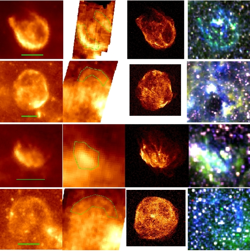
Figure 4.1: Top row, from left to right: N132D at 24 and 70 microns (the region of interest at 70 microns is marked on the image), in the X-rays (broadband, Chandra image) and in the optical (overlay of MCELS images, with [S II], Halpha and [O III] marked in red, green and blue, respectively). Second, third and fourth rows show the same sequence for N49B, N23 and 0453-68.5, respectively. One arc-minute scales are shown on the 24 $\mu$m images.

5 Spitzer Space Telescope Observations of Kepler’s Supernova Remnant: A Detailed Look at the Circumstellar Dust Component

This chapter is reproduced in its entirety from Blair, W.P., Ghavamian, P., Long, K.S., Williams, B.J., Borkowski, K.J., Reynolds, S.P., & Sankrit, R. 2007, ApJ, 662, 998.

5.1 Introduction

Each of the remnants of historical galactic supernovae (SNe) provides a unique and important perspective to our understanding of young supernova remnants (SNRs) and their interaction with the interstellar medium (ISM). SN 1604 is the second youngest galactic SNR (behind Cas A), and was first sighted in October 1604 by Johannes Kepler and others. Kepler was not the first to see the SN, but he published the most detailed account of the SN light curve (Kepler 1606), and largely because of this the SNR has come to be known as Kepler’s SNR. Baade (1943) was the first to recover the optical SNR. It has been well observed at all wavelengths (X-ray: Cassam-Chenaï et al. 2004, Hughes 1999; Radio: DeLaney et al. 2002; Optical: Blair et al. 1991, Sollerman et al. 2003; NIR/IR: Gerardy & Fesen 2001, Douvion et al. 2001; sub-mm: Morgan et al. 2003; and numerous earlier papers referenced therein).

The distance to Kepler’s SNR has been uncertain, with most investigators adopting a value of near 5 kpc, as discussed by Reynoso & Goss (1999). However, Kepler’s SNR lies almost directly toward the galactic center, making the use of H I velocities and a galactic rotation curve very unreliable. Using an HST/ACS image compared to ground-based data, Sankrit et al. (2005) have recently determined a distance of 3.9 (+1.9, -1.4) kpc to Kepler using the proper motion of a filament whose velocity is known with reasonable accuracy (Blair et al. 1991). Since the uncertainty is still rather large, we will adopt a value of 4 kpc in this paper and scale other parameters to this value. The SNR lies $6.8^{\circ}$ off the galactic plane (473 $\rm d_{4}$ pc). With an angular diameter of $\sim$200″, the radius is 1.93 $\rm d_{4}$ pc and the mean expansion velocity has been $\rm\sim 4720~{}d_{4}~{}km~{}s^{-1}$. Since the current velocity of the primary blast wave is $\sim$1660 $\rm\pm 120~{}km~{}s^{-1}$ (Blair et al. 1991; Sankrit et al. 2005), the primary shock has been significantly decelerated over 400 years.

The brightest optical emission is from a region in the WNW, as shown in the images of Blair et al. (1991). Bright [S II] emission indicates slower, denser, radiative shocks. However, more extensive nonradiative emission is present where smoother H$\alpha$ filaments are not accompanied by [S II], for instance, across the N rim and in portions of two centrally-projected regions. We shall refer frequently below to the different character of the radiative and nonradiative emission regions.

Douvion et al. (2001) observed Kepler with the ISOCAM instrument aboard the Infrared Space Observatory (ISO), with an angular resolution of 6″, in a band from 10.7 – 12.0 $\mu$m. Spectra were also obtained between 6.5 and 16 $\mu$m. They found the emission to have a similar morphology to the H$\alpha$ image, but made no distinction between radiative and non-radiative regions. They found almost no line emission to be present and were able to fit their spectra with collisionally heated dust at a fixed temperature, using “astronomical silicate” composition (Draine & Lee 1984), assuming that dust was heated in regions with densities and temperatures consistent with radiative shock emission ($n_{e}\sim(2-10)\times 10^{3}$ cm^-3, $T_{e}\sim 10^{4}$ K. They reported a total dust mass of order $10^{-4}$ $M_{\odot}$.

Kepler’s SNR is the only of the historical SNe from the last millennium whose progenitor type is a matter of serious debate (Blair 2005). The early claim by Baade (1943) of consistency of the historical light curve with a Type Ia SN has been questioned by Doggett & Branch (1985) and Schaefer (1996) among others. The presence of dense, (apparently) N-rich circumstellar material (CSM) surrounding the SNR so high off the galactic plane was taken to indicate pre-SN mass loss from a massive star and hence a core collapse SN (Bandiera 1987). The progenitor could have been a runaway star, which is consistent with the observed morphology (Borkowski et al. 1992; 1994; Velázquez et al. 2006). On the other hand, analyses of X-ray spectra from Exosat (Decourchelle & Ballet 1994), ASCA (Kinugasa & Tsunemi 1999, 2000) and more recently XMM-Newton (Cassam-Chenaï et al. 2004) indicate an overabundance of Fe and Si enhanced ejecta, which is not expected from the explosion of a massive star but instead suggests a Type Ia designation.

At some point in the evolution of a young SNR, some of the SN ejecta may form into interstellar dust of various types, depending on the SN type (e.g. Arendt et al. 1999). Evidence exists for the formation of dust on 1-2 year time scales in core-collapse SN (SN 1987A–McCray 1993 and Bouchet et al. 2004; SN 1999em–Elmhamdi et al. 2003). The large mass of iron produced by Type Ia SNe suggests that grains may form there as well, although direct evidence for this process is scant and timescales are not well known. Dunne et al. (2003) have reported the detection of a large mass of very cold dust in Cas A based on SCUBA (sub-mm) observations, although these conclusions have been called into question (Dwek 2004a,b; Krause et al. 2004). Morgan et al. (2003) have reported SCUBA observations of Kepler’s SNR and claimed a large mass of cold (17 K) dust. A SN blast wave sweeps up gas and dust as it expands, and so any circumstellar or interstellar dust should also be heated, and ultimately sputtered and destroyed by collisions in the post shock region. Hence, young SNRs can in principle be dust-processing laboratories. With the advent of the Spitzer Space Telescope, it is possible to study these effects in unprecedented detail.

Spitzer observations of Magellanic Cloud SNRs are shedding some light on these issues. Borkowski et al. (2006) looked exclusively at four remnants of Type Ia SNe. They found no evidence of dust from the ejecta, but rather emission consistent with heating of ISM dust by the expanding blast wave. B. Williams et al. (2006) selected a group of suspected remnants of core collaspe SNe in the LMC and have found similar results: no obvious dust emission associated with regions of ejecta but dust emission associated with the primary blast wave was prominent. R. Williams et al. (2006) report Spitzer observations of a different sample of LMC SNRs and suggest that, at least in some objects, line emission may dominate over the dust continuum. However, even in these objects, the emission arises at positions consistent with shocked ISM.

In this paper, we report infrared imaging and spectroscopy of Kepler’s SNR using the MIPS and IRAC instruments on Spitzer, obtained as part of a Cycle 1 Guest Observer program (#3413). We find evidence for swept-up dust heated by the primary blast wave, but do not see evidence for the cold dust component reported by Morgan et al. (2003). Modeling of the dust and comparison to observed ratios are used to constrain the allowed plasma conditions in the shocked gas.

5.2 Observations and Data Processing

Below we describe the Spitzer MIPS (Rieke et al. 2004) and IRAC (Fazio et al. 2004) imaging and present the data. The MIPS instrument also has a low resolution spectral energy distribution (SED) spectroscopy mode, and the data obtained on Kepler are described in the subsequent sub-section.

5.2.1 Spitzer Imaging

We observed Kepler’s SNR using MIPS imaging at 24, 70 and 160 $\mu$m, and with all four bands of IRAC (3.6, 4.5, 5.8 and 8.0 $\mu$m). All MIPS photometric imaging used the ‘small’ field size. The 160 $\mu$m band should be most sensitive to the distribution of cold dust, being near the peak of the curve fit by Morgan et al. (2003) to the SCUBA data. Based on the ISO measurements of Douvion et al. (2001), the 24 and 70 $\mu$m MIPS bands and 8 $\mu$m IRAC band should assess the warmer dust component near 120 K.

At 24 $\mu$m we used one cycle and no mapping with a 10 s exposure time. The 70 $\mu$m band used 10 s exposure times, 1 cycle and a 3x1 map for two cycles (step size at 1/2 array for columns and full array for rows). This results in 252 sec integration time and covers the object with room to spare to assess background, and enough overlap to account for the side B problem. The smaller FOV of the 160 $\mu$m band (along with the anomalous block of 5-pixels) required a greater number of positions to cover the desired region. We chose 10 sec exposures and 4 cycles. We then chose mapping with 1x3 for 3 map cycles. This results in an integration time of 252 sec.

We worked with the standard post-BCD reduction data sets for the MIPS imaging data, as retrieved with Leopard from the $\>{\it Spitzer}$ archive. The data have been reprocessed several times over the course of this work, and here we report the S11.0.2 version of the processed data. Figure 1 shows the full field of view MIPS 24 $\mu$m image, which is by far the most sensitive and detailed of the $\>{\it Spitzer}$ images obtained.

Kepler fits within a single IRAC field. Our AOR used the 12 position Reuleaux dither pattern and 2-100 sec frames per pointing to to achieve a 2400 sec integration time in all four bands. We again worked with the post-BCD data sets, which were processed with version S11.4.0. While some SNR emission is apparent in the 8 $\mu$m image, it is difficult to assess the shorter wavelength IRAC images for SNR emission because of stellar contamination.

Hence, to better investigate the extent of SNR emission in the IRAC bands, we have displayed these data in two ways. First, we made three-color images. Figure 2a shows a three-color IRAC image with 8 $\mu$m (red), 5.6 $\mu$m (green), and 3.6 $\mu$m (blue). Stars are white or bluish and the SNR emissions appear orange and yellow. Orange filaments show emission at both 8.0 and 5.6 $\mu$m, but are dominated by the longer wavelength band. Yellow filaments appear to correspond closely with the brighter radiative filaments and indicate relatively stronger emission at 5.6 $\mu$m. Any SNR emission at 3.6 $\mu$m is completely dominated by the longer wavelengths. Figure 2b shows a similar comparison, but using 5.6 $\mu$m as red, 4.5 $\mu$m in green and again 3.6 $\mu$m in blue. Even more so than Fig. 2a, this combination shows only emission from the densest (radiative) optical filaments, which appear as orange (indicating emission in both the 4.5 and 5.6 $\mu$m bands). The two patches of green emission in this Figure adjacent to bright stars indicate instrumental effects in the 4.5 $\mu$m image.

Secondly, we have made difference images of adjacent bands to minimize the effects of stellar contamination. Since SNR emission likely occurs in the band being used for subtraction, these images are not useful for quantitative analysis, but rather for highlighting the overall extent of detected emission. Fig. 2c shows the residual emission when the 5.6 $\mu$m band is subtracted from the 8 $\mu$m image, and Figure 2d shows 4.5 $\mu$m minus 3.6 $\mu$m. While some stellar residuals remain, these two panels confirm the discussion from the three-color Figures above: fairly extensive emission is present at 8$\mu$m, and only a few of the brightest clumpy filaments remain visible at 4.5 $\mu$m.

For comparison, we show a medium scaling of the MIPS 24 $\mu$m image in Figure 2e, and a 0.3 - 0.6 keV energy cut of archival Chandra soft X-ray data in Figure 2f. Comparing Figure 2c and 2e shows that the region visible at 8 $\mu$m corresponds very closely to the brightest regions in the 24 $\mu$m image. There is also tremendous similarity between the softest X-rays and the 8 $\mu$m image. Since the densest regions should be coolest, this confirms to first order that the brightest regions in the 8 and 24 $\mu$m images are largely due to higher densities at these locations.

In Figure 3, we show the MIPS data and some additional comparisons, all on the same scale as the panels of Figure 2. Figure 3a and 3b show hard and soft stretches of the 24 $\mu$m data, respectively, highlighting the faintest and brightest regions detected at 24 $\mu$m. The MIPS 70 $\mu$m data were reprocessed using the GeRT software available from the $\>{\it Spitzer}$ Science Center web site in an attempt to minimize the obvious striping that traverses these data from NNE to SSW. This made a modest improvement in the cosmetic appearance of the 70 $\mu$m image, but the original data set was used for all measurements reported in this paper. The corrected data are shown in Figure 3c. Although the resolution is lower at 70 $\mu$m, it is quite clear that the regions brightest at 70 $\mu$m correspond closely to the brightest emission at 24 $\mu$m. Figure 3d shows the star-subtracted H$\alpha$ image from Blair et al. (1991). The overall extent of the H$\alpha$ emission is quite silimar to the brightest infrared regions, although differences are apparent in the brightest region of radiative filaments in the WNW. Figure 3e shows the MIPS 160 $\mu$m image of the same region as the other panels. No emission is detected above the complex and variable background at 160 $\mu$m. Finally, Figure 3f shows a three color rendition of the Chandra X-ray data. The red shows the same energy cut as in Figure 2f (0.3 - 0.6 keV), green is the energy band 0.75 - 1.2 keV, and blue is a band from 1.64 - 2.02 keV.

5.2.2 MIPS SED Spectroscopy

The MIPS SED spectroscopy mode covers the spectral region from 55 $\mu$m to 95 $\mu$m with a resolution of 15 - 25. The SED aperture covers a region 3.8′ $\times$ 0.32′ and produces a two-dimensional spectral output file with 16 pixels in the spatial direction and 32 pixels in the dispersion direction. A grid of aperture positions covering Kepler’s SNR and an adjacent sky region were observed on 25 Sep. 2005. The spectral grid used a 3′ chop distance in the dispersion direction and an overlapping “a” and “b” position in the spatial direction, covering the northern 2/3rds of the shell (mapping with two overlapping columns and 7 rows). With five cycles, this provided $\sim$300 sec integration times per position.

The primary purpose of the SED spectra was to search for evidence that strong emission lines might be contaminating the broad band imaging, and thus affect their intercomparison. The individual spectra are low in signal and so we chose to sum the data covering the bright NW quadrant of the remnant (grid positions 2b, 3b, 4b, and 5b), using the corresponding sky positions that were furthest removed from SNR emission (sky positions s4b, s5b, s6b and s7b). The aperture positions used are shown in Figure 4, projected onto the 24 $\mu$m image. After summing the object data and subtracting sky, it was clear from displaying the two-dimensional data that the strongest signal was in columns 8 - 12. We collapsed these four columns into the spectrum shown in Fig. 5, which represents the bright NW radiative filaments and a portion of the NW shell. Because of the relatively crude state of SED calibration and software for handling these data, we do not attempt quantitative fits to the resulting spectrum, but rather rely on it to provide a more general description of the mid-IR spectrum.

The SED spectrum is dominated by the tail of the warm dust continuum as it fades to longer wavelengths. There is no evidence at this spectral resolution for the [O I] 63.2 $\mu$m line predicted to be strong in radiative shock models. There may be some indication of the 88.3 $\mu$m line of [O III], but it does not dominate the spectrum. A similar bump near 75 $\mu$m may be due to [N II] 76.5 $\mu$m, which might be consistent with the N overabundance of the shell material as judged from optical spectra, although the wavelength agreement is not very good. In any event, since lines do not dominate in this spectral region where the dust continuum is relatively faint, it is unlikely that line contamination has a signficant effect on the observed 24 $\mu$m flux where the dust emission is much stronger.

This point is strengthened by an IRS spectrum of the NW region by Roellig & Onaka (2004). This spectrum shows a modest emission feature near 26 $\mu$m that they mark as [Fe II] but which may be a blend of this line with [O IV] 25.9 $\mu$m. However, this emission feature makes only a small contribution to the total flux in the 24 $\mu$m band. The IRS spectrum extends down to the IRAC range, showing the dust continuum almost disappearing. In the IRAC 8 $\mu$m bandpass, a moderately strong [Ar II] line appears at 7.0 $\mu$m, accounting for $\sim$ 20% of the total flux. Hence, this is potentially important in considering ratios between the 8 $\mu$m image and other bands, at least for the NW filaments where bright radiative emission is dominating (e.g. Blair et al. 1991).

5.3 Analysis and Modeling

5.3.1 Morphological Comparisons

What is the structure of Kepler’s SNR in the infrared and how does it compare to images at other wavelengths? Although the effective resolutions in the various data sets are different, they are close enough to allow some meaningful intercomparisons. The 24 $\mu$m data are the deepest of the $\>{\it Spitzer}$ data. Scaling to show only the highest surface brightness features, the similarity of Fig. 3b to the IRAC 8 $\mu$m (Fig. 2c) and 70 $\mu$m (Fig. 3c) indicates to first order that the same regions dominate all three bands. The further similarity to the optical H$\alpha$ image (Fig. 3d) and the softest band of X-ray emission (Fig. 2f and red band in Fig. 3f) is striking. Since the majority of the optical emission especially across the northern limb arises from nonradiative shocks associated with the primary blast wave, it is clear that the brightest 8 $\mu$m, 24 $\mu$m, and 70 $\mu$m emissions are associated with this same component. Hence, heating of dust in dense, swept up CSM/ISM is the dominant mechanism operating in Kepler’s SNR.

The morphology of the WNW region including the primary region of bright radiative filaments contains some subtle but important effects. Careful comparison of Fig. 3b and Fig. 3d shows differences between the brightest 24 $\mu$m morphology and the chaotic, more extended emission seen in the H$\alpha$ image. We suggest the 24 $\mu$m image is dominated by emission from the primary blast wave in the moderate density interclump gas, and not the slower radiative shocks in the very dense radiative knots, which are dominated by [S II], [N II], and [O III] line emission (e.g. Blair et al. 1991). The 8 $\mu$m image (Fig. 2c) looks intermediate between the 24 $\mu$m and H$\alpha$ appearance, which is another indicator that line emission from the radiative shocks contributes somewhat at this wavelength, as indicated above in the discussion of the IRS spectrum.

The 24 $\mu$m image scaled to highlight the lowest surface brightness structures (Fig. 3a) is the only of the IR images with sufficient signal to show the entire outer shell of the SNR. A general similarity is seen with the 3-color X-ray image in Fig. 3f, with the exception of the extended ‘ears’ to the WNW and ESE. Similarities to the 6 cm VLA data are apparent (e.g. DeLaney et al. 2002), in particular in the south and along the eastern rim. However differences are also apparent, including a relatively higher IR surface brightness in the NW, along the northern rim, and across the projected middle. The ‘ears’ mentioned above are most apparent in the radio data.

The disagreement in appearance in the projected interior of the shell deserves specific comment. Here an important clue comes from the optical spectroscopy of these central filaments by Blair et al. (1991). The SE central grouping of filaments are significantly red-shifted and thus are a portion of the receding shell of the SNR. In comparison, the NW central filaments are blue-shifted and are part of the approaching shell of the SNR. These filaments have direct counterparts in the soft X-ray band, but the association with the higher energy X-ray bands is less clear. The approaching filaments have no counterpart in the radio data, and while there is faint radio emission at the projected position of the SE central grouping of filaments, the morphologies are different. Hence, it is not clear whether any of the central radio emission is correlated with either the optical or bright IR emissions in these regions.

In Figure 6, we show a different kind of morphological comparsion. This color composite, star-subtracted image shows Kepler’s SNR as viewed by NASA’s three Great Observatories, with $\>{\it Spitzer}$ 24 $\mu$m data in red, $\>{\it Hubble}$ H$\alpha$ in yellow, $\>{\it Chandra}$ 0.3 - 1.0 keV emission in green, and harder 2 - 10 keV $\>{\it Chandra}$ emission in blue. This image provides a combination of physical information and some subtle affects due to differing spatial resolution of the data sets used. The $\>{\it Hubble}$ data have the highest spatial resolution, but highlight the fact that the optical emission arises in knotty, dense structures being encountered by the primary blast wave. These filaments are bathed in the glow of the IR component, which arises from dust heated by the blast wave. The X-ray emission in the north extends out to the optical limb and stops. The red rim around the top is largely an artifact of the lower resolution of the 24 $\mu$m data and the stretch applied to this component of the image. (As we indicated in the discussion above, the brightest 24 $\mu$m emission is coincident with the shock front position.) However, the larger extension of the red emission in the NW appears to be a real effect.

The distribution of the two X-ray components in Fig. 6 is quite interesting. The harder X-rays (blue) primarily arise in sychrotron emission at the shock front, and are seen most clearly along the southern and eastern limbs. The softer X-ray component is dominated by thermal emission from Si and Fe rich ejecta (e.g. Cassam-Chenaï et al. 2004). In the south, this component lies directly interior to the blue component. In the north, this component largely fills in between the northern limb emission and the centrally-projected emission regions. Note the distinct absence of red emission in the green regions, which indicates no significant warm dust emission coincident with regions of ejecta.

5.3.2 Derivation of IR Fluxes and Ratios

We now turn to more quantitative information, concentrating first on the 24 $\mu$m and 70 $\mu$m data sets, where contamination of the SNR emission by stars is not a significant problem. We derived the total fluxes at these two wavelengths using the following method. Because the post-BCD data are in units of MJy $\rm sr^{-1}$, we extract regions of pixels corresponding to the object, and use the known post BCD pixel sizes (from the file headers) and number of pixels included in each region to scale appropriately to total fluxes. We similarly extract representative regions of background surrounding the SNR region (as allowed by field coverage) and average these to determine the most appropriate overall background levels to subtract. Using this technique, we obtain total fluxes at 70 and 24 $\mu$m of 4.90 Jy and 9.5 Jy, respectively, and thus a ratio of 70/24 $\mu$m of 0.52.

Our total flux at 70 $\mu$m appears to disagree with published IRAS fluxes at 60 $\mu$m (range from 7.1 - 10.5 Jy), summarized by Saken et al. (1992, their Table 6), although our derived 24 $\mu$m flux lies within the range listed (8.1 - 11.7 Jy) at IRAS 25 $\mu$m. The apparent disagreement arises simply from the differing bandpasses used. Bandpasses for IRAS are broader than for Spitzer, and thus would encompass more flux at a given wavelength. To confirm this, we integrated the output spectrum from the dust model described below for the entire remnant over the IRAS 60 $\mu$m bandpass and obtained an “expected” 60 $\mu$m flux of $\sim$8 Jy. A corresponding exercise for the Spitzer 70 $\mu$m band predicts a flux of  5 Jy.

In addition to the total fluxes, we have determined the 24 and 70 $\mu$m fluxes for several sub-regions of the remnant to search for variations in these ratios that might arise due to different shock or other parameters. We have also measured fluxes from relevant regions of the IRAC 8 $\mu$m image, although stellar contamination is a more significant problem for these data. Figure 7 shows the extraction regions projected onto the relevant images. These figures also define the nomenclature we will use below to reference the regions.

Because Spitzer’s optics provide images at or near the diffraction limit for all wavelengths, the resolution in images from various instruments differs by roughly the ratio of wavelengths. The angular resolutions of various images range from 2″ at 8 $\mu$m, to 6.2″ at 24 $\mu$m, 18″ at 70 $\mu$m, and 41″ at 160 $\mu$m. For determination of flux ratios from various regions of the SNR, it is necessary to convolve the higher-resolution image of interest to the resolution of the lower-resolution image. For the 8/24 $\mu$m ratios, we convolve the 8 $\mu$m image to the resolution of that at 24 $\mu$m, and for the 24/70 $\mu$m ratios, we convolve the 24 $\mu$m image to the resolution of that at 70 $\mu$m. We used contributed software by K. Gordon (U. Arizona) distributed by the SSC to convolve the images, using kernels for convolving 24 $\mu$m images to the same PSF as 70 $\mu$m, and similarly for 8 $\mu$m to 24 $\mu$m. These kernels are slightly temperature-dependent; we used versions appropriate for 100 K. Though we do not expect blackbody spectral shapes, this value is close to the appproximate grain temperatures reported by Douvion et al. (2001). In each case, the higher-resolution images were resampled onto a grid identical to that of the lower resolution image, using AIPS (Astronomical Image Processing System) task HGEOM. These are the images shown in Figure 7.

The extraction regions were defined to select physically associated regions of emission so that the results could be compared. We displayed and aligned the 24 and 70 $\mu$m images using the display tool ds9. We also displayed the optical H$\alpha$ and other images on the same scale for reference and comparison while defining regions. The defined 24 and 70 $\mu$m regions are shown in Figure 7a-c, and details are given at the top of Table 1. Object position O1 enclosed the region of bright radiative emission in the NW, position O2 enclosed the entire bright NW rim at 24 $\mu$m. Note that by differencing these two positions, the area corresponding to just the relatively bright nonradiative portion of the NW rim can be extracted. O3 samples the northern (mainly) nonradiative rim, and O4 and O5 enclose the two centrally-projected regions of knotty filaments.

Background regions were identified to the north and south of the remnant to account for the gradient observed in the background from north to south. Some backgrounds were defined specifically for use with the 70 $\mu$m image in an attempt to better account for the significant striping in this image. For each object position, the most appropriate backgrounds were summed and scaled to the size of the object region being measured. Specifically, we used the following regions as background at 70 $\mu$m: For positions O1 and O2 in Figure 7a-c, background regions B1 and B5 were averaged and used. For positions O3 and O5, background regions B2 and B4 were used. And for position O4, background regions B2 and B3 were used. At 24 $\mu$m we simply used regions B1, B2 and B4, which do not overlap SNR emission.

The signal in each sampled region was measured using the FUNtools package that interfaces with ds9. As with the total flux estimates, it is necessary to multiply the total signal above background measured in a region by the pixel scale (sr $\rm pixel^{-1}$). Thus, ratios use the same spatial object regions, even though the pixel sizes varied. The region fluxes and ratios between 24 and 70 $\mu$m are provided in Table 2. Only small differences are obtained. In particular, the similarity in ratio between O1 and O3, or O1 and the difference between O2-O1, indicates that there is no significant difference in 70/24 $\mu$m ratio between bright radiative and nonradiative regions. This is in keeping with the earlier discussion about the IRS and SED spectra, where these emissions are dominated by the main blast wave.

We have also derived ratios of regions between 8 $\mu$m and 24 $\mu$m using a similar technique, although for somewhat modified spatial regions than used with the 70/24 $\mu$m ratios. The defined 8 and 24 $\mu$m regions are shown in Figure 7d-f, and details are given at the bottom of Table 1. This comparison is complicated by the faintness of the 8 $\mu$m emission, by the presence of many more stars at 8 $\mu$m, and by the difference in resolution between the images. Because of potential contamination of the 8 $\mu$m image by the [Ar II] 7.0 $\mu$m line seen by Roellig & Onaka (2004), the derived ratios may be skewed toward slightly higher 8/24 $\mu$m ratios than true. On the other hand, any relative changes in the ratio should be real.

For the 8 $\mu$m to 24 $\mu$m comparison, positions O1 and O2 isolate the two brightest regions of radiative optical filaments in the NW. Position O3 samples the so-called ‘bump’ region, which includes both radiative and nonradiative optical emission in the NNW. O4 provides the cleanest sampling of nonradiative shock emission on the northern rim. O5 and O6 sample two regions of central emission knots, but are smaller regions than measured above for the 70/24 $\mu$m ratio. Again, optical data suggests a mixture of radiative and nonradiative shocks in these regions. Stars have largely been avoided, with the exception of position O6, for which it was impossible to totally exclude stars from the selected region. At 8 and 24 $\mu$m, we simply averaged all three of the background regions shown and applied this as representative to all positions.

We have applied recommended photometric corrections for diffuse sources appropriate for the 8 $\mu$m band, as described in the IRAC section of the SSC website. This correction for sources large compared to the calibration aperture for point sources (12″) is a factor of 0.74, which has been applied to measured fluxes and backgrounds for this band. However, this correction is sufficiently poorly known that an additional uncertainty of order 10% is introduced. Any relative changes in the 8/24 $\mu$m ratio should remain valid, however.

The derived 8/24 $\mu$m ratios are summarized in Table 3. Comparing the measurements at positions O1 and O2 to O4, we see higher ratios at the strongly radiative positions, indicative of contamination of the 8 $\mu$m image by line emission (likely [Ar II], as indicated in the IRS spectrum discussion above). Hence, the O4 measurement likely represents the most accurate assessment of the 8/24 $\mu$m dust continuum. It is unclear without IRS data whether the higher ratios observed at O3, O5, and O6 are due to variations in the dust continuum or due to significant IR line emission from the optically faint radiative filaments in these regions.

We have not color-corrected the observed fluxes reported in the Tables. Our model fluxes have been produced by integration of the calculated spectrum over the Spitzer bandpasses at 24 and 70 $\mu$m. Since Spitzer fluxes are calibrated by comparison with stars whose spectra at 24 $\mu$m and longward are well-approximated by the Rayleigh-Jeans limit of a blackbody, we have assumed a $\lambda^{-2}$ spectrum and calculated what Spitzer would report for the flux at the nominal frequency for each band. That is, we have converted our model fluxes into “Spitzer space” before computing model ratios, rather than color-correcting observed fluxes. However, such corrections would not be large in any case. Our shock models that reproduce the observed flux ratios give grain temperatures between 75 and 95 K. While the spectra are not exact blackbodies, color corrections for a 70 K blackbody are less than 10% at both 24 and 70 $\mu$m, as reported in the MIPS Data Handbook (v3.0, p. 29); at 100 K, they are less than 7% at both wavelengths. For IRAC, color corrections are reported in the IRAC Data Handbook only down to blackbody temperatures of 200 K. For that temperature, corrections are less than 20% for both Channels 3 and 4. We believe that overall calibration errors, estimated in the Spitzer Observing Manual, Sec. 8.3.3 (p. 355) to be 10% for extended sources at 24 $\mu$m and 15–20% at 70$\mu$m, will dominate the errors at those bands. We can also estimate internal statistical errors from the pixel-to-pixel dispersion in the background; these errors are negligibly small compared to those due to calibration. We adopt conservative overall error estimates of 10% at 24 $\mu$m and 20% at 70 $\mu$m.

In addition to deriving region ratios as described above, we also created a ratio map from the convolved 24 $\mu$m image and the 70 $\mu$m image as follows. First, we measured a mean background from most of the region on the image not occupied by the source (avoiding obvious point sources), and subtracted that value, at each wavelength. Then we blanked the convolved 24 $\mu$m image below 10 MJy/sr, a level corresponding to about 20% of peak, which left all obvious structure intact. (The off-source rms fluctuation level was 0.6 MJy/sr.) At 70 $\mu$m, a much noisier image, the off-source rms was about 1.6 MJy/sr; we blanked below 5 MJy/sr, about three times this value. The point of the blanking is to make sure that only pixels whose measured fluxes are highly significant at both wavelengths are used to compute ratios. We then generated the ratio image shown in Fig. 8.

Figure 8 shows several features of interest. First, a general anticorrelation of ratio with 24 $\mu$m brightness indicates that hotter (lower 70/24 $\mu$m ratio) regions are brighter. Second, the minima in the ratio are actually offset from the 24 $\mu$m brightness peaks slightly. Third, the western region of bright radiative shocks appears to have somewhat different ratio. The range of pixels in the image is about 0.3 – 0.8, with a broad maximum around 0.45 and most pixels between 0.35 and 0.5, consistent with the values measured in regions shown in Table 2. Higher ratios in the fainter regions is the primary reason the total 70/24 $\mu$m = 0.52 even though most of the brighter regions have lower ratios.

5.3.3 Grain Emission Modeling

The morphological comparisons across different wavelengths show a clear correlation between the soft X-ray images and IR images at all three MIPS wavelengths, 8, 24 and 70 $\mu$m. We thus attribute emission from Kepler in these bands to shocked interstellar and circumstellar dust, heated by the hot, X-ray emitting plasma in the primary blast wave (Dwek & Arendt 1992). Collisions with energetic electrons and ions heat dust grains to $\sim 100K$, where they emit thermal radiation visible to Spitzer’s mid-IR instruments. In addition to heating, the ions in the plasma sputter dust grains, rearranging the grain-size distribution by destroying small grains and sputtering material off of large grains. We employ computer models of collisionally heated dust to explain what is seen in Kepler, identical to what was done for Type Ia SNRs (Borkowski et al. 2006) and core-collapse SNRs (B. Williams et al. 2006) for SNRs in the Large Magellanic Cloud. Our models use as input an arbitrary grain-size distribution, grain type (astronomical silicates, carbonaceous, etc.), proton and electron density $n_{p}$ and $n_{e}$, ion and electron temperature $T_{i}$ and $T_{e}$, and shock age (or sputtering time scale) $\tau_{p}=\int_{0}^{t}n_{p}dt$. The model is based on the code described by Borkowski et al. (1994) in the context of photon-heated dust in planetary nebula Abell 30, and augmented to allow for heating by energetic particles in hot plasmas.

Because little is known about the surroundings of Kepler, we adopt a power-law grain size distribution with index $\alpha$ = -3.5 and an exponential cutoff. We use a range of 100 grain sizes from 1 nm to 0.5 $\mu$m. We also use only astronomical silicates. This is consistent with past efforts to model dust emission from Kepler (Douvion et al. 2001). We use bulk optical constants for astronomical silicates from Draine & Lee (1984). Energy deposition rates for electrons and protons were calculated according to Dwek (1987) and Dwek & Smith (1996). Because small grains are stochastically heated and have large temperature fluctuations as a function of time, we must account for the increased radiation produced by such transient heating. We use the method described by Guhathakurta & Draine (1989) for this purpose.

It is also necessary to model sputtering for all grains, since sputtering alters the grain size distribution downstream of the shock. Sputtering rates for grains in a hot plasma are taken from Bianchi et al. (2005). Small grains can actually experience an enhancement in sputtering due to the ion knocking off atoms not only from the front of the grain, but also from the sides or the back. We have included such enhancements in our models, with enhanced sputtering yields described by Jurac et al. (1998). Sputtering is very important in the dense CSM environment of Kepler, and results in the efficient destruction of small grains in the postshock gas and very significant modification of the preshock grain size distribution. Even MIPS fluxes and their ratios depend on the shock sputtering age, but because emission in these bands is mostly produced by relatively large grains with moderate temperature fluctuations, sputtering effects are less extreme than at shorter wavelengths. We consider our dust models reliable for modeling MIPS fluxes and their ratios. Thermal fluctuations are particularly important in very small grains, which reradiate their energy at short wavelengths, so sputtering dramatically reduces the amount of radiation in the IRAC bands.

Contrary to expectations, the 8 $\mu$m emission is much stronger than predicted by our models. While we do not include PAHs in our modeling code, they are not likely to be present in large quantities given the absence of their distinctive spectral features in IRS spectra (Roellig & Onaka 2004). However, the model does not account for several physical effects likely to be important for very small grains, such as discrete heating (i.e., discrete energy losses as an electron or proton traverses a grain), and corrections to heating and sputtering rates required when particle mean free paths are much greater than grain radius. For these reasons, we have not attempted to model the 8/24 $\mu$m flux ratios shown in Table 3. A great deal of theoretical work remains to be done before the wealth of data produced by Spitzer can be used effectively to understand the properties of small grains.

For modeling an outward moving shock wave, we have used a one-dimensional plane-shock approximation. The plane-shock model assumes a constant temperature, but superimposes regions of varying sputtering timescale from zero up to a specified shock age (Dwek et al. 1996). The shock model effectively varies the product of density and time behind the shock, allowing us to account for material that has just been shocked and material that was shocked long ago, since these will experience different amounts of sputtering. The output of our models is a single spectrum, which is produced by superimposing spectra of many different grain sizes. Since we do not model observed spectra directly, we can only fit flux ratios from photometric measurements. We focus here on reproducing the observed 70/24 $\mu$m ratios.

We constructed a grid of dust models to explore the parameter spaces of temperature and density, covering electron temperatures $kT_{e}$ from 0.03 to 10 keV and electron densities $n_{e}$ ranging from 3 to $10^{3}$ cm^-3. We assumed that ion and electron temperatures are equal. The output of the grid was $\sim 300$ separate models with varying $n$, $T$, and $\tau_{p}$, the shock sputtering age. (Since $\tau_{p}$ inherently contains $n_{p}$, and $n_{p}$ is related by a constant factor to $n_{e}$, $\tau_{p}$ is varied from model to model. See Borkowski et al. 2006.) We divide the actual age of Kepler by 3 to approximate an “effective shock age” for Kepler, which was used in the models. The factor of $1/3$ arises from applying results of a spherical blast wave model to the plane-shock calculation (Borkowski et al. 2001).

For each of the 300 models, a 70/24 $\mu$m ratio was calculated from the output spectrum, and the value of the ratio was plotted on a two-dimensional color-coded plot as a function of electron density and pressure (see Figure 9). We then added contours to the plot which correspond to measured values of the 70/24 $\mu$m ratio from the MIPS images. The three contours are the highest and lowest measured region values (regions O3 and O5, 0.40 and 0.30, respectively; see Table 2), and the value of 0.52 appropriate for the spatially-integrated fluxes. The plasma conditions for the nonradiative regions of Kepler’s SNR can be contained for the most part between these contours. Our nonradiative shock models are not applicable at high densities and low temperatures (toward the lower right corner of Fig. 9) because of the onset of radiative cooling. Shocks with an age of 400 yr and solar abundances. for instance, become radiative to the right of the line shown in the lower right corner of Figure 9. We used postshock cooling ages tabulated by Hartigan et al. (1987) to draw this line in the electron temperature–pressure plane.

At low densities (near the left boundary of Fig. 9), our models with equal ion and electron temperatures overestimate the 70/24 $\mu$m flux ratio. In this region of plasma parameters, shocks are fast and ion temperatures are generally larger than electron temperatures. Heating of grains by ions becomes relatively more important, resulting in increased grain temperatures and lower 70/24 $\mu$m flux ratios relative to shocks with equal ion and electron temperatures. We estimated an electron temperature for the northwest portion of the remnant, where Sankrit et al. (2005) determined a shock speed of 1660 $\rm km~{}s^{-1}$. We used a simple model for the ion-electron equilibration through Coulomb collisions behind the shock. From this we derived a $T_{e}$ of 1.2 keV (in the absence of significant collisionless electron heating and assuming a shock age of $\sim 150$ yr). A shock model with a postshock electron density of 22 cm^-3 reproduces the measured ratio of 0.40; we mark its position by a star in Figure 9. (Without sputtering, this ratio would have been equal to 0.31.) A noticeable displacement of this model from the middle contour is caused by additional heating by ions in the more sophisticated model with unequal ion and electron temperatures used for the Balmer-dominated shock in the north. Grain temperatures in this model vary from 75 K to 95 K.

Our estimate of a typical electron density in dust-emitting regions of $n_{e}\sim 20$ cm^-3 is in reasonable agreement with other estimates, such as the estimate of $7-12$ cm^-3 in the central optical knots (Blair et al. 1991). It should characterize the bulk of the shocked CSM around Kepler, although higher postshock electron densities and lower temperatures (and hence lower shock speeds) are also possible because contours of constant 70/24 $\mu$m ratio approximately coincide with lines of constant pressure on the right hand side of Figure 9. While nonradiative Balmer-dominated shocks with speeds less than 1660 km s^-1 have not been measured to date in Kepler, the highly inhomogeneous optical and X-ray morphologies suggest that plasma conditions in the shocked CSM may vary greatly with position within the remnant. It is likely that shocks are present with velocities less than seen in the Balmer-dominated shocks but more than seen in radiative shocks. Shocks with such intermediate velocities are best studied at X-ray wavelengths, and a future analysis of the CSM in Kepler based on a new long Chandra observation is in progress (Reynolds et al. 2006). It is also likely that fast nonradiative shocks in the south and east travel through gas with densities much less than 20 cm^-3; the current MIPS 70 $\mu$m data and optical observations are not sensitive enough to study these shocks in much detail.

Our derived value of $n_{e}T_{e}=3\times 10^{8}$ cm^-3 K ($n_{e}kT_{e}=26$ cm^-3 keV) is in the pressure range considered by Douvion et al. (2001). However, based on the morphological resemblance between the 24 $\mu$m image and the nonradiative optical emission, a lower density and higher temperature better characterize the typical dust emitting regions.

5.3.4 Total Dust Mass and Dust/Gas Ratio

The spatially-integrated IR spectrum of Kepler is produced by grains of widely varying sizes immersed in inhomogeneous plasmas. This results in a wide range of grain temperatures, making determination of a total dust mass model dependent because of the extreme sensitivity of the radiated IR power to the grain temperature. In Appendix A, we estimate the shocked CSM X-ray emission measure in Kepler using a simple plane shock model with a mean temperature of 5 keV and ionization age of $10^{11}$ cm^-3 s, without any collisionless heating at the shock front but allowing for energy transfer from ions to electrons through Coulomb collisions. Emission measure-averaged ion and electron temperatures are 8.9 keV and 1.4 keV in this shock model. The only remaining free parameters in the model are a postshock electron density $n_{e}$ and a total dust mass. We obtain $n_{e}=13$ cm^-3 by matching the measured spatially-integrated 70/24 $\mu$m flux ratio of 0.52. (There is a nonnegligible contribution to grain heating from hot ions in this fast shock; as can be inferred from Figure 9, simpler shock models with equal ion and electron temperature of 1.4 keV predict a slighty higher 70/24 $\mu$m ratio of 0.58.) We then derive a total dust mass of $5.4\times 10^{-4}$ $M_{\odot}$ from the measured spatially-integrated MIPS fluxes.

We obtain nearly the same mass when we use instead plasma conditions assumed by Douvion et al. (2001), $n_{e}=6000$ cm^-3 and $kT_{e}=0.0043$ keV, corresponding to a model spectrum shown by a solid line in their Figure 3, and based on fits to IRAS and ISO observations. (Douvion et al. 2001 quote a smaller dust mass of $1-2\times 10^{-4}$ $M_{\odot}$, appropriate for their simple model with hot silicate dust at temperature of 107.5 K, significantly hotter than dust in our models.) This agreement between two different mass determinations based on independent data and very different assumed plasma conditions is encouraging; a future more detailed spatially-resolved joint study of Spitzer and Chandra data should provide us with a refined dust mass determination. The mass of $5.4\times 10^{-4}$ $M_{\odot}$ refers to dust currently present in the shocked CSM. Most (78%) of dust was destroyed in our fast shock model, implying an initial (preshock) dust mass of 0.0024 $M_{\odot}$. Because dust destruction rates depend sensitively on the assumed shock speed and its age, our current estimate of the preshock dust mass is rather uncertain.

The total IR flux in the plane shock model discussed above is $1.4\times 10^{-9}$ ergs s^-1 cm^-2, in good agreement with IRAS-based fluxes of $1.3\times 10^{-9}$ ergs s^-1 cm^-2 and $1.6\times 10^{-9}$ ergs s^-1 cm^-2 listed by Dwek (1987) and Arendt (1989), respectively. The IR luminosity is $2.8\times 10^{36}$ ergs s^-1. Kepler is a low-luminosity object when compared with SNRs for which this type of analysis has been done with IRAS (e.g., Saken et al. 1992). More recently, Borkowski et al. (2006) derived total luminosities for two of the four SNRs from Type Ia SNe in their study, and B. Williams et al. (2006) derived luminosities for all four of their sample of SNRs from core-collapse SNe in the Large Magellanic Cloud. Of these six remnants, only SNR 0548-70.4 has a luminosity lower than Kepler, and even it is comparable at $2\times 10^{36}$ ergs s^-1. This SNR is, however, several times larger (and thus likely older) than Kepler. Indeed, most of the remnants in these two studies have luminosities much higher than Kepler.

A specific object of interest for comparison is Tycho, a Type Ia SNR of comparable age located at a 2 kpc distance. The IR flux of Tycho is $5\times 10^{-9}$ ergs cm^-2 s^-1 (Arendt 1989), so its IR luminosity is comparable to Kepler. Dust in Tycho is much cooler than in Kepler (Arendt 1989, Saken et al. 1992), consistent with a much lower ISM density around Tycho. SNR 0509-67.5, one of the remnants studied by Borkowski et al. (2006) in the LMC, appears very similar to Tycho. While observations of light echoes (Rest et al. 2005) have placed the age of this SNR at $\sim$ 400 yr, a high shock speed deduced from optical and UV observations of Balmer-dominated shocks (Ghavamian et al. 2007) implies a low ambient ISM density. Its MIPS 24 $\mu$m flux is 16.7 mJy, about 2–4 times lower than what Tycho or Kepler would have at a distance of 50 kpc. An upper limit to its dust mass is 0.0011 $M_{\odot}$, and SNR 0509-67.5 is likely less luminous in the IR than Tycho or Kepler.

Determination of the dust/gas mass ratio requires knowledge of the shocked CSM gas mass. Using an X-ray emission measure of 10 $M_{\odot}$ cm^-3 (Appendix A) and $n_{e}=13$ cm^-3, we derive a total shocked CSM mass in Kepler of 0.77 $M_{\odot}$. This is in good agreement with a shocked CSM mass of 0.95 $M_{\odot}$ derived from ASCA observations (Kinugasa & Tsunemi 1999), after scaling their results to the 4 kpc distance used here and using an electron density of 13 cm^-3. The hydrodynamical model of Borkowski et al. (1992, 1994), based on the massive core-collapse runaway progenitor scenario of Bandiera (1987), requires $\sim 1~{}M_{\odot}$, also in reasonable agreement with the present mass estimate. Recent hydrodynamical models of Velázquez et al. (2006), based on a Type Ia progenitor scenario, require several $M_{\odot}$ of shocked CSM. But Velázquez et al. (2006) used collisional equilibrium ionization X-ray spectral models, which underestimate X-ray emission by an order of magnitude or more for young SNRs (Hamilton et al. 1983; see also Appendix A), resulting in an excessive estimate of the shocked mass by a comparable factor.

Combined with the dust mass from above of 0.0024 $M_{\odot}$, we arrive at a dust-to-gas mass ratio for the CSM surrounding Kepler of 0.003. This is lower than the generally accepted figure for the Galaxy (e.g., Weingartner & Draine 2001) by a factor of several. Since the dust in Kepler appears to have originated in some kind of a stellar outflow, the lower dust content may be related to this and not a characteristic of the general ISM in the region. Kepler’s dust/gas ratio is higher by a factor of several than found for SNRs in the Magellanic Clouds (Borkowski et al. 2006; B. Williams et al. 2006; Bouchet et al. 2006), most likely because of the high (near or above solar) metallicity of its SN progenitor compared with the $\sim$0.4 solar LMC abundance.

5.3.5 North-South Density Gradient

A number of indicators imply a potential difference in preshock density from north to south across the Kepler region. The difference in the surface brightness of the north rim compared to the south rim is one indicator, and the effect may be visible directly from the background in Fig. 1 and the appearance of the 160 $\mu$m image in Fig. 2e. The south rim is only faintly visible at 24 $\mu$m, while the north rim is extremely bright. We believe the 24 $\mu$m is dominated by dust emission, although some contribution from emission lines cannot be ruled out without spectra. Under this assumption, we took a small region of the southern rim and an equal-sized region of the northern rim that is dominated by nonradiative shocks and measured the flux from both regions at 24 $\mu$m. The regions were arcs following the shape of the rim, approximately 23″ in thickness and 75″ in length. The south region follows the faint southern rim at a declination of approximately -21:31:04 (J2000). We found a north/south ratio of 24 $\mu$m fluxes of $\sim$30. A possible explanation for this contrast is that the shocks are encountering regions of different density.

We have made several estimates of the density contrast necessary to produce the observed intensity ratio. First, we assume that the dust-to-gas mass ratio in the two regions is the same (although we make no a priori assumptions about what that ratio must be). We do not assume equal amounts of swept-up material in the two regions, but rather simply vary the gas density (and dust mass accordingly) in the models and assume the same shock speed (and thus the same temperature) for both regions. This method reproduces the observed flux difference with a modest density contrast of only a factor of $\sim$4.5. It should be noted that these are all post-shock densities.

As an alternative approach to this problem, one can relax the requirement that the shock speeds be equivalent in the two regions, since a variation in density should cause variations in shock speed. We repeated the calculations for several different shock speeds in the south region, while keeping the north region constant at 1660 km s^-1, and a density of $n_{e}=19.5$ cm^-3. We calculated electron and proton temperatures for the south region with these different shock speeds assuming no equilibration at the shock front, and used these different temperatures to predict dust emission at 24 $\mu$m. In these models, the density contrast required is only weakly dependent on shock speed. While grains are heated to hotter temperatures in faster shocks, the amount of destruction of grains also increases. Overall, we find that for a reasonable range of shock speeds up to 3000 km s^-1, a post-shock density contrast between 4 and 7 times lower in the south (and accordingly 4–7 times less dust present) can reproduce the observed ratio. The density contrast increases with faster shock speeds.

As a third approach, we consider the remnant to be in pressure equilibrium. Keeping the density and shock speed in the northern region constant with the values mentioned above, we varied the shock speed in the south and derived density from the pressure equilibrium expression $n_{N}V_{N}^{2}\equiv n_{S}V_{S}^{2}$, where subscripts N and S refer to the north and south regions, respectively. Under this constraint, we determined the shock speed required to reproduce the observed 24 $\mu$m flux ratio, again assuming a constant dust-to-gas mass ratio. We find that a shock with speed $\sim$5000 km s^-1, and thus a density of $\sim$ 2.1 cm^-3 can account for the difference in fluxes coming from the two regions. This is a density contrast of 9.1. Because 5000 km s^-1 is much higher than inferred from other indicators, this contrast in density is considered an upper limit. The predicted 70/24 $\mu$m flux ratio in the south region is $\sim$ 1.2, which is significantly higher than in the brighter regions of the remnant, but consistent with the idea that the dust in that region is cooler. It is also consistent in a general sense with the higher overall average 70/24 $\mu$m ratio of 0.52. Since the these models are only constrained by the fluxes observed at 24 $\mu$m in the south, these results should be considered tentative. Detailed mid-infrared spectroscopy will be required to investigate this issue further.

5.3.6 Whither the Cold Dust Component?

Morgan et al. (2003; hereafter M03) have recently reported excess emission in Kepler using SCUBA 450 and 850 $\mu$m observations. They model this as a cold astronomical silicate dust component from ejecta ($T_{d}$ = 17 K), inferring as much as a solar mass of material in this component. Dwek (2004a) proposes a differing interpretation, arguing instead for a component at $T_{d}$ = 8 K and a much lower mass of dust in the form of Fe needles. He supports the general possibility of a cold dust component related to the ejecta, pointing to a similar component identified in Cas A (Dwek 2004b), but the amount of mass involved would be much lower than inferred by M03. Douvion et al. (1991) would not have been able to detect this cold component.

Our MIPS 160 $\mu$m image shown in Figure 3 is directly relevant to this discussion since this wavelength is close to the peak of the cold component curve predicted by M03 (see their Figure 2). No emission related to the SNR shell or interior is detected at 160 $\mu$m, although the background is patchy and there appears to be a general gradient of intensity from NE toward the SW in the image.

To derive an upper limit at 160 $\mu$m, we extracted emission from the region corresponding to the SNR location (judging from an aligned overlay of the 24$\mu$m image) and from nearby background regions, as described above for the 24 and 70 $\mu$m images. Background levels to the north and east of the SNR are at a higher level than the average from the object location, while the background level in the south is slightly below the object region average. The observed field of view is very close to the western edge of the SNR, but the background in that region appears to be comparable to that in the south. To be conservative, we apply the southern background level to the entire object, which will over-estimate any contribution from the SNR. The resulting upper limit we derive is 0.8 Jy at 160 $\mu$m, which is approximately a factor of 10 below the value predicted by M03 from the SCUBA-based model. Hence, our $\>{\it Spitzer}$ 160 $\mu$m data do not confirm the M03 cold-dust picture. This fairly conservative upper limit does not rule out the idea of Fe needles as discussed by Dwek (2004a), but the presence of any such component in Kepler has been argued against on theoretical grounds (Gomez et al. 2005). Even if present, any such component in Kepler’s SNR would contain well below 0.1 solar mass, and would not require a massive precursor star as in the M03 interpretation.

5.3.7 Synchrotron Emission

X-ray synchrotron emission has been reported for Kepler: thin filaments seen in the eastern “ear” extension (Bamba et al. 2005), broader emission from the SE quadrant (Cassam-Chenaï et al. 2004), and an extension of the integrated flux to hard X-rays (Allen, Gotthelf, & Petre 1999). The X-ray fluxes demand a steepening of the extrapolated radio spectrum; if that steepening occurs at shorter than IR wavelengths, IR synchrotron emission should be present with a morphology identical to the radio and at readily extrapolated brightness levels. While the average radio spectral index of Kepler is –0.71 ($S_{\nu}\propto\nu^{\alpha}$) (DeLaney et al. 2002), higher-frequency archival radio data imply a value of –0.59 (Reynolds & Ellison 1992). This concave-up curvature, or hardening to shorter wavelengths, can occur for electrons accelerated in a shock modified by the pressure of accelerated ions (Ellison & Reynolds 1991). If we extrapolate from images at cm wavelengths (e.g., DeLaney et al. 2002) with this value, we predict surface brightnesses at 3.6 $\mu$m in the range 0.6 – 1.1 $\mu$Jy arcsec^-2 (or $(2.5-4.8)\times 10^{-2}$ MJy sr^-1). Our 3.6 $\mu$m image shows only a faint hint of any emission associated with Kepler. In particular, there is no apparent emission in the SE quadrant. Typical brightness levels are 0.4 – 0.5 MJy sr^-1, or 10 – 20 times the extrapolated synchrotron flux. Even with very significant hardening of the spectrum above 10 GHz, the 3.6 $\mu$m data are not constraining the presence of synchrotron emission. In particular, the regions identified by Bamba et al. (2005) and Cassam-Chenaï et al. (2004), the SE quadrant and the eastern “ear,” are very faint in IR in general. The western “ear” may also harbor X-ray synchrotron emission, and it too is fainter at 24 $\mu$m relative to the rest of the shell emission. Far more sensitive IR observations would be necessary to detect synchrotron emission.

5.4 Discussion

Of the historical SNe, Kepler’s remains enigmatic because a clear determination of the SN type (and thus precursor star) has proven elusive. Claims of evidence supporting both a massive precursor (core collapse SN type) or a white dwarf precursor (Type Ia SN) abound in the literature over the last decade or more. In this section, we discuss this issue and highlight new insights that may help resolve this dichotomy.

Firstly, since not all SN ejecta can form into dust, the claim by M03 of a solar mass or more of cold dust in Kepler was an indication of even more ejecta mass and hence a massive precursor star. The negative detection at 160 $\mu$m here points to an apparent problem with the SCUBA result, presumably due to the complex and variable background observed in this region. Hence, a massive precursor is not required by the IR data.

Another indication pointing toward a massive precursor star has been the overabundance of nitrogen in the optically-emitting filaments, which are thought to represent dense knots of CSM being overrun by the blast wave. We have run a small grid of shock models using the current version of the shock code described by Raymond (1979) and Hartigan et al. (1987) for comparison with the optical spectrum of knot ‘D3,’ a bright, radiative shock knot presented by Blair et al. (1991, their Table 2). We find that the main features of this spectrum can be matched with a model similar to model E100 of Hartigan et al. (1987), but with the N abundance increased by 0.5 dex. This is indeed a significant enhancement over solar abundance.

However, solar abundances are the wrong reference point. At a distance of $\sim$4 kpc and galactic coordinate G4.5+6.8, Kepler’s SNR is nearly half way to the galactic center. Rudolph et al. (2006) provide a summary of galactic abundance gradients, and for nitrogen find an increase of $\sim$0.3 dex for the assumed distance of Kepler’s SNR. Additionally, inspection of their Figure 4 shows that the scatter in observed points around the best fit line for the gradient readily encompasses the required value of 0.5 dex enhancement in nitrogen at Kepler’s distance from the galactic center. While the nitrogen abundance around Kepler’s SNR may be enhanced relative to its local surroundings, it is not required, and certainly the magnitude of any enhancement is considerably less than has been recognized previously.

We note, however, that this in no way negates the fact that the presence of dense material surrounding Kepler’s SN is surprising for an object nearly 500 pc off the galactic plane. This material must have its origin in either the precursor star, or the precursor system (if a binary of some type was involved). Canonical wisdom says that core collapse precursors are massive stars, and massive stars shed material via stellar winds prior to exploding. Type Ia SNe are thought to arise from white dwarf stars that are pushed over the Chandrasekhar limit, although the exact details of the precursor system that gives arise to this are still widely debated (e.g. Livio & Riess 2003, and references therein). The absence of hydrogen lines in the spectra of Type Ia SNe is taken as evidence for CO white dwarfs with little or no photospheric hydrogen, and certainly little if any CSM.

Improved statistics on extragalactic SNe, however, are finding exceptions to this general scenario. A small but growing class of bona fide (confirmed with spectra) Type Ia SNe has been found that show narrow hydrogen lines at late times, indicating the presence of a CSM component close to these objects. SN 2002ic is a recent example of this phenomenon. Some authors dub these objects Type Ia/IIn (e.g., a Type Ia with narrow hydrogen lines; Kotak et al. 2004) while others denote such objects as a new SN type, IIa (i.e., a Type Ia with hydrogen lines; Deng et al. 2004). Whatever the designation, these objects demonstrate that some SNIa explosions can occur in regions with significant CSM, albeit at distances closer in to the SN than inferred for Kepler. Any such close in component near Kepler’s SN, if present, would have long since been overrun by the blast wave.

Direct evidence for the presence of (presumably) CSM material around another Type Ia SN was provided by Hubble Space Telescope images of light echoes around SN 1998bu (Garnavich et al. 2001; Patat 2005). Among several light echoes detected in this SN, there is an echo generated by scattering off dust located closer that 10 pc to the SN. At the same time, SN 1998bu has one of the most stringent upper limits on the density of the stellar wind (Panagia et al. 2006). The presence of a detached CSM (or perhaps an ISM shell swept-up by winds of the SN progenitor) is likely in this nearby SN. These and similar observations open up the possibility that Kepler’s SNR represents a local example of this phenomenon.

Finally, it should be noted that recent detailed X-ray observations and modeling (Kinugasa & Tsunemi 1999; Cassam-Chenaï et al. 2004) are consistent with Si and Fe-rich ejecta, but show no evidence for other enhancements seen in core collapse SNRs such as Cas A (Hughes et al. 2000; Hwang & Laming 2003). The temperature structure inferred within the X-ray ejecta, with Fe K peaking interior to Fe L is reminscent of Type Ia SNRs such as SN1006 and Tycho (Hwang & Gotthelf 1997; DeCourchelle et al. 2001). These early results are strengthened almost to the point of certainty by a recent deep Chandra X-ray exposure on Kepler that will allow a detailed assessment of abundances within the ejecta of Kepler (Reynolds et al. 2006). The preponderance of evidence from the X-rays now points toward a Type Ia origin for the precursor of Kepler’s SNR.

If Kepler represents a SNIa explosion in a region with significant CSM, it would be important from two directions: If plausible models are put forward that can explain a Type Ia with significant CSM, applying them to Kepler’s SNR may provide a stringent test because of its proximity and wealth of supporting observational data. On the other hand, Kepler is only one object, and observations of additional extragalactic examples of SNIa’s with CSM in various forms may provide important clues about the frequency and/or the progenitor population of such explosions (e.g. Mannucci 2005).

5.5 Conclusions

We have presented Spitzer imaging of Kepler’s supernova remnant at 3.6, 4.5, 5.8, 8, 24, 70, and 160 $\mu$m wavelengths and compared with data from other wave bands. Emission associated with the remnant is obvious at all except 160 $\mu$m, but emission in the two shortest-wavelength IRAC bands is visible only at the locations of bright optical radiative shocks in the WNW. However, at 24 $\mu$m, the entire periphery of the remnant can be seen, along with emission seen, at least in projection, toward the interior.

To summarize, we find:

• The 24 $\mu$m emission is well correlated with the outer blast wave as delineated by soft X-ray emission and by nonradiative (Balmer-dominated) shocks seen in the optical. This is clearly emission from dust heated by collisions in the X-ray emitting material. It is not well correlated either with ejecta emission (shown by strong Fe L-shell emission in X-rays) or with dense regions containing radiative shocks. In particular, we find no evidence for dust newly formed within the ejecta material.

• The emission at 8 $\mu$m largely resembles that of the brightest regions at 24 $\mu$m, although contamination by line emission in the 8 $\mu$m is apparent in the radiative shock regions. This similarity indicates that even short-wavelength emission originates from the same grain population as that at longer wavelengths. However, current models are not yet able to describe emission from the implied population of small grains.

• The emission at 70 $\mu$m is similar to that at 24 $\mu$m, but a higher background makes it difficult to discern the fainter southern half of the remnant. Where both 70 $\mu$m and 24 $\mu$m emission can be seen, 70/24 $\mu$m flux ratios for discrete regions range from 0.37 to 0.49. Lower values, implying higher temperatures, are correlated with brighter regions. A total object average ratio of 0.52 implies that the fainter regions tend toward higher values of this ratio.

• The SED spectrum indicates that lines make at most a small contribution between 55 and 95 $\mu$m. The spectrum, along with the absence of emission at 160 $\mu$m, rules out the presence of large amounts of cold dust.

• Dust models using a power-law grain size distribution and including grain heating and sputtering by X-ray emitting gas can explain observed 70/24 $\mu$m flux ratios with sensible parameters. The models give gas densities of 10 – 20 cm^-3. The range of observed ratios can be explained by ranges of temperature and density of different regions in rough pressure equilibrium.

• We find a total dust mass of about $5.4\times 10^{-4}\ M_{\odot}$ after sputtering, and infer an original mass of about $2.4\times 10^{-3}\ M_{\odot}$. With an estimate of shocked gas mass from X-ray data, we infer an original dust/gas ratio of about $3\times 10^{-3}$, lower by a factor of several than normally assumed for the Galaxy, as has been found for several other supernova remnants.

• We find that a moderate density contrast in the range of $\sim$4 – 9 is required to explain the brightness variations observed between the north and south rims of the remnant at 24 $\mu$m, depending somewhat on the assumptions and models applied.

• We suggest the preponderance of current evidence from optical, X-ray, and infrared data and modelling now points toward a Type Ia supernova, albeit in a region of significant surrounding CSM/ISM, especially for an object so far off the galactic plane. A possible similarity to several extragalactic Type Ia supernovas with narrow hydrogen lines at late times is pointed out.

Data from the Spitzer Space Telescope clearly demand more sophisticated grain modeling. The absence of large quantities of newly formed dust challenges models hypothesizing such dust formation in the SN ejecta. However, the heated dust from the circumstellar medium heated by the blast wave can provide useful diagnostics of plasma conditions.

Table 5.1: Aperture Parameters for Region Extractions

Region	$\alpha$ (2000)	$\delta$ (2000)	Semi-Major	Semi-Minor	PA (∘)
			Axis (″)	Axis (″)
24 $\micron$ to 70 $\micron$:
Object 1	17:30:35.76	-21:28:44.5	21.4	30.0	192.9
Object 2	17:30:36.73	-21:28:27.2	20.8	50.2	218.9
Object 3	17:30:41.81	-21:27:54.6	39.8	18.4	182.9
Object 4	17:30:43.51	-21:29:48.0	31.2	20.2	182.9
Object 5	17:30:39.93	-21:29:17.9	28.8	17.2	182.9
Background 1	17:30:36.82	-21:27:05.2	18.5	27.9	186.3
Background 2	17:30:42.96	-21:27:03.2	39.8	18.4	182.9
Background 3	17:30:41.91	-21:31:45.7	34.0	21.6	186.3
Background 4	17:30:38.24	-21:32:15.7	35.1	17.2	182.9
Background 5	17:30:34.05	-21:31:40.2	22.3	48.7	186.3
8 $\micron$ to 24 $\micron$:
Object 1	17:30:35.81	-21:28:55.0	7.2	7.8	93.2
Object 2	17:30:36.28	-21:28:33.7	10.2	10.2	0
Object 3	17:30:38.14	-21:27:59.7	7.2	7.2	0
Object 4	17:30:42.61	-21:27:51.8	9.6	15.6	103.2
Object 5	17:30:42.61	-21:27:51.8	9.6	15.6	103.2
Object 6	17:30:40.09	-21:29:21.8	9.0	14.4	103.2
Background 1	17:30:35.92	-21:27:34.5	29.4	14.4	138.2
Background 2	17:30:42.07	-21:27:12.3	10.2	20.4	43.2
Background 3	17:30:40.28	-21:31:23.9	12.0	17.4	93.2

Table 5.2 – MIPS 70/24 $\mu$m Regions Summary Region^a Net 70 $\mu$m^b Flux Net 24 $\mu$m Flux^b 70/24 Ratio mJy mJy O1 778 2133 0.36 O2 1171 3125 0.37 O2 $-$ O1 394 992 0.40 O3 412 1032 0.40 O4 349 886 0.39 O5 242 766 0.30

Notes: (a) Refer to Figure 7a-c for region definitions. (b) Net fluxes have been background-subtracted as described in the text.

Table 3 – MIPS 8/24 $\mu$m Regions Summary Region^a Net 8 $\mu$m^b Flux Net 24 $\mu$m Flux^b 8/24 Ratio mJy mJy O1 10.4 409 0.025 O2 16.5 571 0.029 O3 6.9 242 0.029 O4 6.9 314 0.022 O5 5.4 228 0.024 O6 11.7 339 0.035

Notes: (a) Refer to Figure 7d-f for region definitions. (b) Net fluxes have been background-subtracted as described in the text.

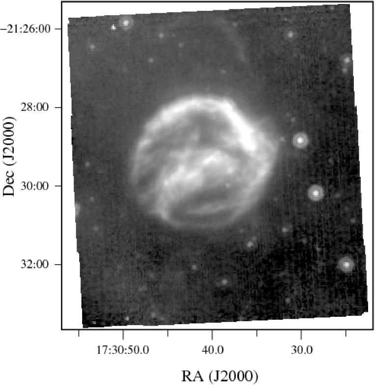
Figure 5.1: Full field of view MIPS 24 $\mu$m image of Kepler’s SNR. Scaling is set to a compromise level to show the overall structure to best advantage. The 24 $\mu$m image is by far the deepest and most detailed of the Spitzer images.

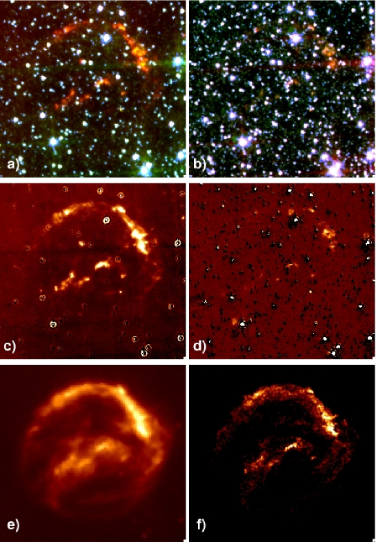
Figure 5.2: A six-panel color figure concentrating on the IRAC images and their comparison to other wavelength bands. Panel a shows a three-color IRAC image with 8 $\mu$m in red, 5.6 $\mu$m in green and 3.6 $\mu$m in blue. Panel b is similar, but for 5.6 $\mu$m in red, 4.5 $\mu$m in green, and 3.6 $\mu$m in blue. The orange color of the SNR filaments indicates emission in both 4.5 and 5.6 $\mu$m, but only from the brightest filaments seen at 8 $\mu$m. Panel c is a difference image of 8 $\mu$m minus 5.6 $\mu$m, scaled to show the extent of faint emission at 8 $\mu$m. Panel d shows the 4.5 $\mu$m minus 3.6 $\mu$m difference image. Panel e shows the 24 $\mu$m MIPS image from Fig. 1 to the same scale as the other images. The 8 $\mu$m image closely tracks the brightest regions at 24 $\mu$m. Panel f shows the soft band (0.3 - 0.6 keV) Chandra image from archival data, which again looks astonishingly like the 8 $\mu$m image in panel c. All images are aligned and scaled exactly the same.

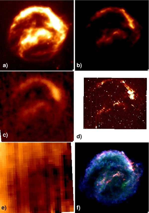
Figure 5.3: A six-panel color figure concentrating on the MIPS images and their comparison to other wavelength bands. Panels a and b show the MIPS 24 $\mu$m data with a hard stretch and a soft stretch, respectively, to show the full dynamic range of these data. Panel c shows the MIPS 70 $\mu$m data after running through the GeRT software to improve the appearance of the background. Panel e shows the MIPS 160 $\mu$m data for the same field of view, although no SNR emission is actually seen at this wavelength. Panel d shows the star-subtracted H$\alpha$ image from Blair et al. (1991). Panel f shows a three-color representation of the Chandra data for Kepler, with the red being 0.3 - 0.6 keV (as in Fig. 2f), green being 0.75 - 1.2 keV, and blue being 1.64 - 2.02 keV.

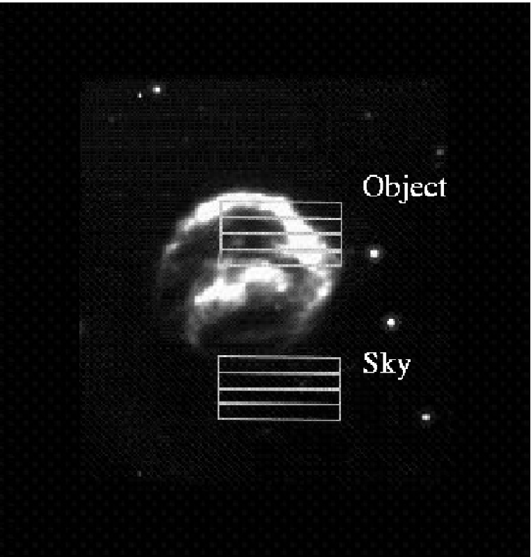
Figure 5.4: SED apertures selected for assessing the bright NW radiative emission and the sky background, projected on the 24 $\mu$m image.

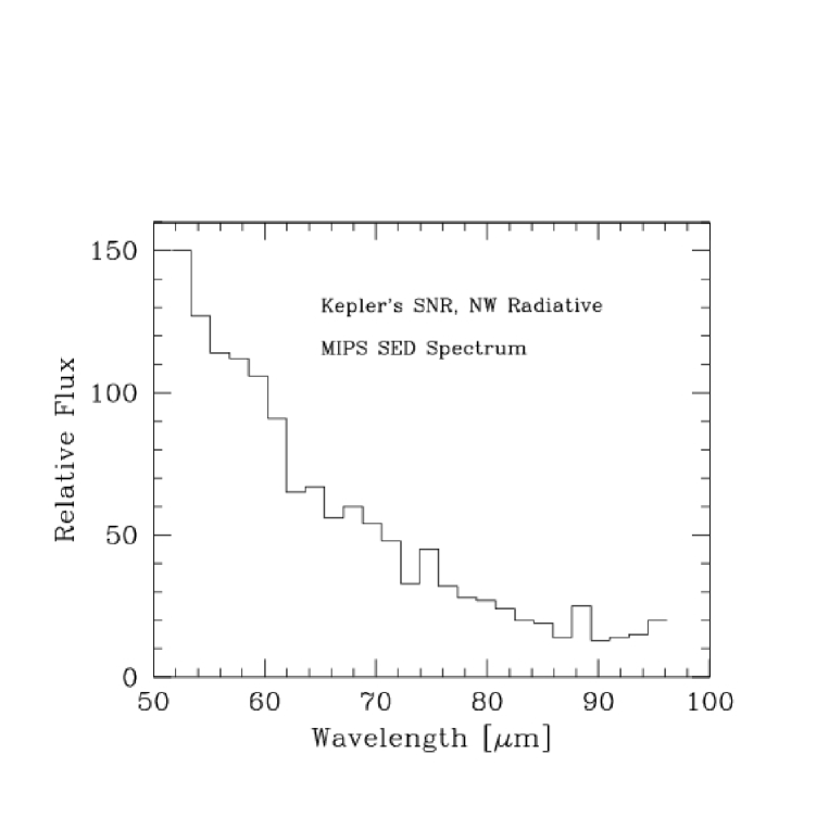
Figure 5.5: Background subtracted SED 55 - 95 $\mu$m spectrum of the NW region of Kepler’s SNR, as indicated in Figure 4.

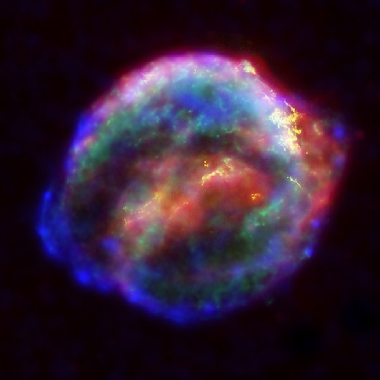
Figure 5.6: A color view of Kepler showing data from $\>{\it Spitzer}$ 24 $\mu$m (red), $\>{\it Hubble}$ ACS H$\alpha$ (yellow), and $\>{\it Chandra}$ medium (blue) and soft (green) X-ray emission bands. Despite the differing intrinsic resolutions of the various data sets, they have been carefully coaligned. A $\>{\it Hubble}$ continuum-band image was used to subtract the stars from this image. See text for details.

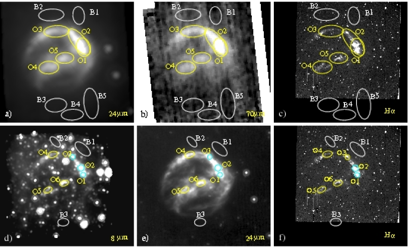
Figure 5.7: This figure shows the object and background extraction regions selected for determining ratios between 24 and 70 $\mu$m (panels a and b) and between 8 and 24 $\mu$m (panels d and e). For reference, the regions are also projected onto the optical H$\alpha$ image from Blair et al. (1991) in panels c and f. Note that the images shown in panel a and d are the versions that have been convolved to the lower resolution image. Also, panel b shows the original (non-GeRT-corrected) 70 $\mu$m image. The labels are used in the text and Tables 5-2 and 5-3.

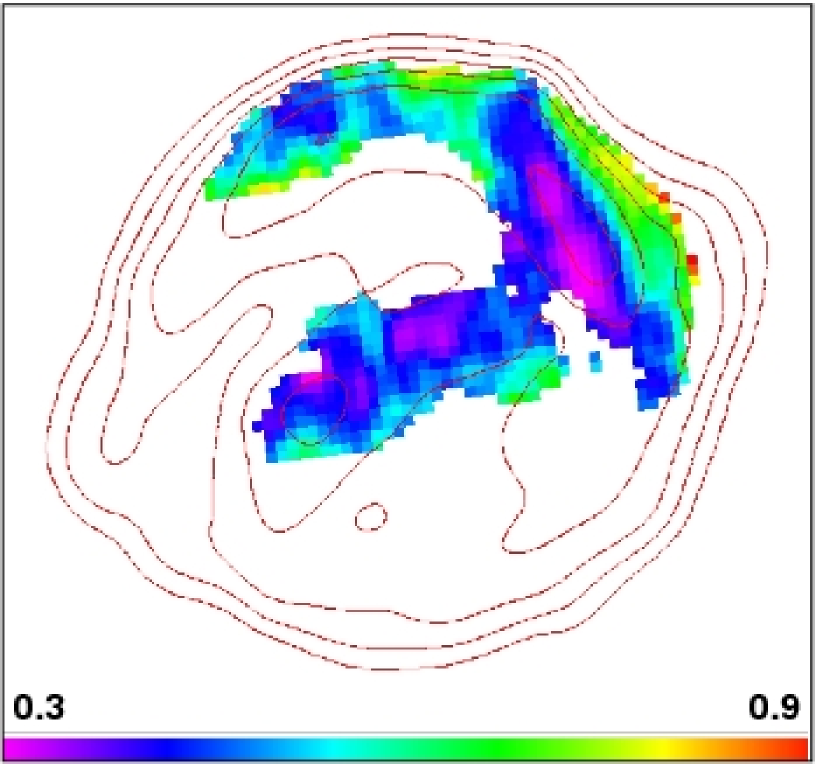
Figure 5.8: A ratio image of the 70 $\mu$m and 24 $\mu$m data, where only the regions with significant signal have been kept. The color bar provides an indication of the measured ratio, ranging from 0.28 to 0.9. A simple contour from the 24 $\mu$m image is shown for comparison. Note the lower values of the ratio in the regions of brightest emission, indicating they are somewhat warmer.

Figure 5.9: The 70/24 $\mu$m MIPS flux ratio as a function of electron density and pressure for plane shock dust models discussed in the text. The background color scale indicates 70/24 $\mu$m ratio, as indicated by the color bar at right. Dashed lines are lines of constant temperature. The solid magenta diagonal line at lower right indicates where the modeled shocks would become radiative, assuming solar abundance models and an age of 400 years. Three solid curves are lines of constant 70/24 MIPS flux ratios, 0.30, 0.40, and 0.52 (from top to bottom), encompassing measured ratios listed in Table 2 and the spatially-integrated ratio. Position of a Balmer-dominated fast (1660 km s^-1) shock in the north is marked by a star.

6 Ejecta, Dust, and Synchrotron Radiation in SNR B0540-69.3: A More Crab-like Remnant than the Crab

This chapter is reproduced in its entirety from Williams, B.J., Borkowski, K.J., Reynolds, S.P., Raymond, J.C., Long, K.S., Morse, J.A., Blair, W.P., Ghavamian, P., Sankrit, R., Hendrick, S.P., Smith, R.C., Points, S., & Winkler, P.F. 2008, ApJ, 687, 1054.

6.1 Introduction

Many core-collapse supernovae (SNe) leave behind a neutron star as a compact remnant. Some of these neutron stars are active pulsars which inflate a bubble of relativistic particles and magnetic fields confined by the ejecta or interstellar medium (ISM), known as a pulsar-wind nebula. The combination of a shell supernova remnant (SNR) and associated pulsar-wind nebula can allow the investigation of various issues of importance in supernova and pulsar physics, including pulsar kicks, ejecta structure and composition, and particle acceleration at relativistic shocks. Pulsar-wind nebulae serve as calorimeters for pulsar spindown energy loss, and as test systems to study the behavior of relativistic shocks where the pulsar wind is thermalized. We know of few cases of a “normal” radio and X-ray shell supernova remnant containing an active pulsar and synchrotron nebula. Probably the best known such ideal case is the Large Magellanic Cloud remnant B0540-69.3 (or “0540” for short). 0540 is also one of a highly exclusive group of “oxygen-rich” SNRs, a group that includes Cas A, Puppis A, G292+1.8, 1E0102-72.3, and N132D.

Theoretical studies of PWNe have either concentrated on the gross evolution, assuming a homogeneous nebula (Rees & Gunn, 1974; Pacini & Salvati, 1973; Reynolds & Chevalier, 1984) or the detailed spatial structure, neglecting evolution (Kennel & Coroniti, 1984). Since the advent of the new generation of X-ray observatories, the study of PWNe has accelerated, with the identification of many new objects and more detailed information on known ones (see Gaensler & Slane 2006 for a recent review). Chevalier (2005) modeled PWNe for different assumptions about the ejecta profiles into which they expand, to relate properties of supernovae to those of the PWNe.

PWNe produce extremely broad-band spectral-energy distributions (SEDs), well described in various frequency regimes with power laws. Most PWNe are observed in radio and X-rays; only a few are detected optically (here as in many other ways the Crab Nebula is an exception), and almost nothing is known about infrared or ultraviolet spectra. Typical radio spectra are featureless, and are well described by power-laws with spectral indices $\alpha<0.3$ ($S_{\nu}\propto\nu^{-\alpha}$), with X-ray indices steeper by 0.5 – 1.3 (see data in Chevalier 2005). Since simple models of synchrotron losses predict a steepening of exactly 0.5, they lack some essential physics, which may be constrained if the complete spectrum is known. Galactic PWNe are all found close to the Galactic plane, where they suffer from extinction in optical and UV and confusion in IR. Filling in the SED between radio and X-rays can best be done with a high-latitude object. For this reason as for many others, 0540 is an interesting target.

0540 was first catalogued as a radio source of unknown nature, a minor feature on a 408 MHz map of the 30 Dor region made with the Molonglo telescope (Le Marne, 1968). Mathewson & Clarke (1973) first classified it as a supernova remnant on the basis of its steep radio spectrum, although their optical survey did not detect it. Early reports associated 0540 with the H$\alpha$ emission nebula N 158A (Henize, 1956), though that object is $3^{\prime}$ from the centroid of the early radio positions (which could be localized to better than $10^{\prime\prime}$). The absence of strong H$\alpha$ emission from 0540 further demonstrates that the association with N 158A is erroneous. Subsequent radio observations (Milne, Caswell, & Haynes, 1980) gave an improved spectral index of $-0.44$, typical for a shell supernova remnant. The first indication of something unusual was the X-ray detection (Long & Helfand, 1979) with the Einstein Observatory, in which 0540 was the third brightest X-ray remnant in the LMC. The X-ray spectrum was shown to be featureless by Clark et al. (1982) with the Einstein Solid-State Spectrometer. The first optical detection was reported by Mathewson et al. (1980), motivated by pre-publication reports of the observations of Clark et al (1982). Mathewson et al. did not see H$\alpha$ but instead a spectacular ring in [O III] of $8^{\prime\prime}$ diameter, with a smaller ring in fainter [N II] emission ($4^{\prime\prime}$ diameter) and no appreciable Balmer emission. In addition to classifying 0540 as an “oxygen-rich” SNR, Mathewson et al. (1980) also reported spectroscopic observations indicating expansion speeds of order 1500 km s^-1. The discovery of the 50 ms X-ray pulsar (Seward, Harnden, & Helfand, 1984) and optical synchrotron nebula (Chanan, Helfand, & Reynolds, 1990) added to the complexity and interest of the system. The optical emission was shown definitively to be synchrotron by the discovery of polarization (Chanan & Helfand, 1990). The pulsar spindown timescale $P/2{\dot{P}}$ is about 1660 yr (Seward, Harnden, & Helfand, 1984), somewhat longer than the kinematic age estimate resulting from dividing the radius ($4^{\prime\prime}=1$ pc at our assumed distance of 50 kpc) by the expansion speed of about 1500 km s^-1, which yields a value of $\sim 700$ yr. The pulsar spindown luminosity is $1.5\times 10^{38}$ erg s^-1.

Reynolds (1985) modeled 0540 with the formalism of Reynolds & Chevalier (1984), with the pulsar driving an accelerating synchrotron nebula into the inner edge of expanding ejecta. At that time, there were no more than hints of extended structure that could be identified with the outer blast wave. Reynolds (1985) found that the current radio, optical, and X-ray observations could be explained without requiring extreme values for the pulsar initial energy or other parameters. He deduced an initial pulsar period of about $30\pm 8$ ms, that is, relatively slow, and concluded that the true age of 0540 was between 800 and 1100 yr, somewhat longer than the kinematic age due to the pulsar-driven acceleration.

Up to this time, all observations were consistent with 0540 being a standard Crab-like remnant (i.e., a nonthermal center-brightened radio and X-ray nebula surrounding a pulsar), except for the hint of larger-scale structure from radio images and from X-ray observations (Seward, Harnden, & Helfand, 1984). Definitive information on the structure came from higher-resolution radio observations with the Australia Telescope (Manchester, Staveley-Smith, & Kesteven, 1993) which showed a clear radio shell with diameter about $65^{\prime\prime}$ surrounding a radio nebula with size (about $5^{\prime\prime}$ FWHM) comparable to the bright X-ray nebula and [O III] ring. The shell has a radio spectral index $\alpha$ of about $-0.4$, while the central nebula has $\alpha=-0.25$. At this point it was clear that 0540 is even more Crab-like than the Crab, as it possesses a clear outer blast wave interacting with surrounding material, so that we could be sure that the interior PWN is interacting with the inner SN ejecta as in Reynolds & Chevalier (1984). X-ray emission from the blast wave was confirmed with Chandra observations (Hwang et al., 2001); the emission is brightest in the W and SW, like the radio. Spectral fits indicated abundances typical of the LMC, with a temperature of order 4 keV (for a Sedov blast wave model) and ionization timescale $\tau\equiv n_{e}t=3.7\times 10^{10}$ cm^-3 s, though spectral differences are apparent in different regions, and a hard component may be called for.

The most thorough optical spectroscopic study to date was reported by Kirshner et al. (1989). They confirmed the high velocities (FWZI $\sim 2800$ km s^-1), and reported weak H$\alpha$ emission. The average centroid of SNR lines (as opposed to narrower lines from a nearby H II region) was shifted by $+370$ km s^-1. No [Ne III] was reported ($<1.5$ % of [O III]); they concluded that this was a real abundance deficit rather than a temperature or density effect. A detailed study by Serafimovich et al. (2004), focusing on the optical nonthermal continuum, revised the reddening and optical slope to give a power-law index in the optical of $\alpha_{o}=-1.07.$ Recent observations by Morse et al. (2006) report the discovery of faint [O III] emission extending to a radius of $8^{\prime\prime}$, with a velocity of 1650 km s^-1. They find the centroid of this velocity component to be the same as that of the LMC, so that a large peculiar velocity of the system is not required.

Chevalier (2005) modeled 0540, along with several other PWNe, with the goal of learning more about the SN explosion. He obtained several results for a simple dynamical model of a PWN expanding into ejecta of various density profiles driven by a pulsar of given power. He interpreted 0540 as the result of a SN Ib/c, an exploding Wolf-Rayet star, with the prediction of a lack of significant emission from hydrogen. However, recent optical observations by Serafimovich et al. (2004) and Morse et al. (2006) have detected hydrogen. In light of this, it is now believed (Chevalier, 2006) that 0540 is the result of a type IIP supernova.

The infrared observations of 0540, which was detected by the Infrared Space Observatory (ISO) (Gallant & Tuffs, 1999), presented in this paper promise to advance our understanding on several fronts. The outline of our paper is as follows: In section 6.2, we describe the observations and data reduction, and results are given in section 6.3. In section 6.4.1, we discuss a general picture of the PWN, and sections 6.4.2 and 6.4.3 discuss in detail the line emission and dust continuum emission, respectively. In section 6.4.4, we discuss the origin of the O-rich clumps, whose existence we posit in section 4.2. Section 6.5 serves as a summary of our findings.

6.2 Observations and Data Reduction

During Cycle 1 of Spitzer observations, we obtained pointed observations of 0540 with the Infrared Array Camera (IRAC) and the Multiband Imaging Photometer for Spitzer (MIPS) as part of a survey of $\sim 40$ known supernova remnants in the Large and Small Magellanic Clouds (Borkowski, et al., 2006; Williams et al., 2006). Our IRAC observations (28 November 2004) consisted of a dither pattern of 5 pointings with a frame time of 30 seconds for each frame. This pattern was used for all 4 IRAC channels. Our MIPS observations (7 March 2005) differed based on the module used. At 24 $\mu$m, we mapped the region with 42 overlapping pointings of 10 seconds each. At 70 $\mu$m, we mapped the remnant with 94 pointings of 10 seconds each. At 160 $\mu$m, we mapped the region with 252 pointings of 3.15 seconds. Since 0540 was not detected at 160 $\mu$m, we do not discuss 160 $\mu$m data here. Both the Basic Calibrated Data (BCD) and Post-BCD products were processed with version S14.4 of the PBCD pipeline. We then used the Spitzer Science Center (SSC) contributed software package MOPEX to “clean up” the images, although the improvements were minimal. MOPEX was able to remove some of the streaks caused by bright stars in the IRAC images of the region.

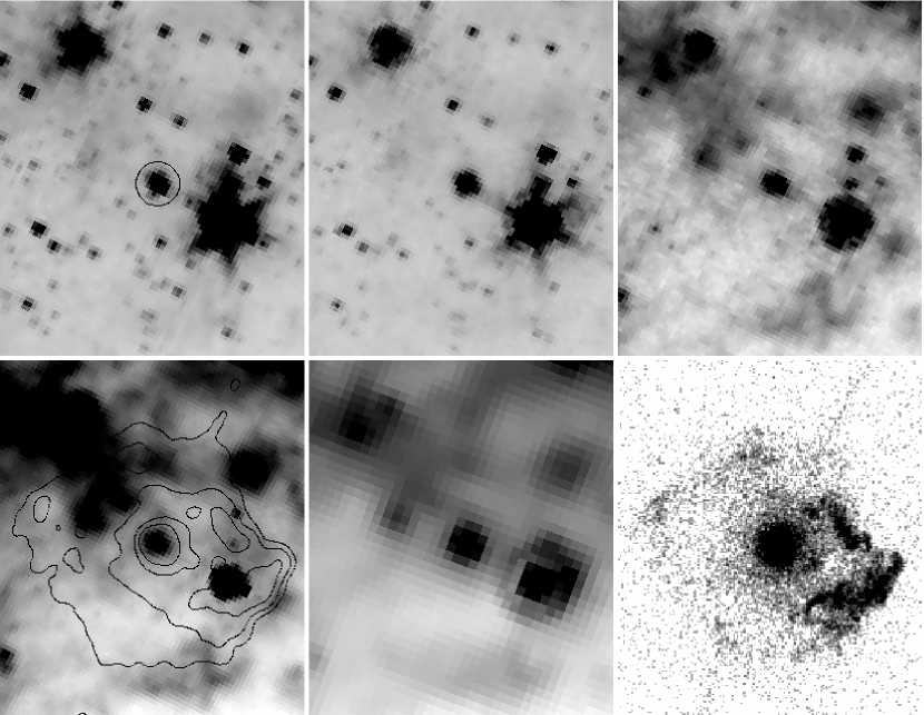
Figure 6.1: Images of PWN 0540-69.3. Each image is approximately 100 arcseconds across. Left to Right, Top to Bottom: IRAC Chs. 1-4 (3.6, 4.5, 5.6, and 8.0 $\mu$m, respectively), MIPS 24 $\mu$m, Chandra broadband X-ray image. The location of the PWN is marked with a circle in the IRAC Ch.1 image, and X-ray contours are overlaid on the IRAC Ch.4 image.

Our images of the source are shown in Figure 6.1. With a radius of $\sim 4^{\prime\prime}$, the PWN is resolved by Spitzer, and it clearly stands out from the background in IRAC and MIPS 24 $\mu$m bands. In IRAC ch. 3 & 4 (5.8 & 8.0 $\mu$m), as well as MIPS 24 $\mu$m, there is a hint of a shell around the nebula, at approximately $30^{\prime\prime}$. We considered the possibility that this shell is related to the SNR, perhaps the collisionally heated dust from the outer blast wave, as we have observed in several other SNRs. However, the morphology of the IR shell does not correspond with any features in the X-ray or radio shell. Spectroscopy of the shell shows it to be virtually identical to the surrounding background unrelated to the remnant, so we are forced to conclude that its apparent relation to the SNR is coincidental.

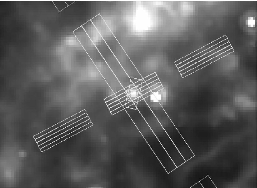
Figure 6.2: Coverage of IRS slits overlaid on MIPS 24 $\mu$m image.

In Cycle 2, we obtained spectroscopic pointings for 0540 using all four instruments of the Infrared Spectrograph (IRS). Our observations were done between 8-10 July 2005. We used the spectral mapping mode for the low-resolution modules, and staring mode for the high-resolution echelle modules. Figure  6.2 shows our coverage of the PWN with IRS overlaid on our MIPS 24 $\mu$m image. For the short-wavelength, low-resolution module (SL) we obtained 5 parallel pointings with each of the two orders, with a step direction of $3.5"$ perpendicular to the dispersion direction of the slit. A total of 480 seconds (2 cycles of 240 s) was obtained for each slit position. For the long-wavelength, low-resolution (LL) module, we obtained 3 parallel pointings for each order with a step direction of $10.5"$ perpendicular to the dispersion direction. A single cycle of 120 seconds was used for LL. Since we are primarily interested in determining the shape of the continuum from the low resolution spectra, it was important to obtain spectra of the local background as well as the source. Figure 6.1 illustrates the complex nature of the local background and the difficulty of accurate background subtraction. Because our source is only $\sim 8^{\prime\prime}$ in diameter, we were able to extract background spectra from not only the parallel slit pointings, but also from different parts of the slit containing the source. We downloaded the Post-BCD data, pipeline version S15, from the SSC. We used the Spitzer IRS Custom Extraction (SPICE) software provided by the SSC to extract our spectra. Although the PWN is slightly extended, it is close enough to a point source, especially at longer wavelengths, to use the point source extraction mode in SPICE.

In order to determine line profiles and strengths from the source itself, we also obtained pointings with both the short-wavelength, high-resolution (SH) and long-wavelength, high-resolution (LH) modules in staring mode. For these pointings, we centered the echelle spectrographs only on the source, without a dedicated background pointing. Since staring mode automatically provides 2 nod positions for each pointing, we averaged the two to obtain a single spectrum for SH and a single spectrum for LH. For SH, we used 3 ramp cycles of 480 seconds each, for a total of 1440 s. The same total integration time was obtained for LH, but was broken up into 6 cycles of 240 s each.

6.3 Results

6.3.1 Flux Extraction

0540-69.3 is located close to the 30 Doradus region of the LMC, and thus is in a region of high infrared background. For our IRAC and MIPS images, we simply used an annular background region to subtract off the background flux from the PWN. Because the nebula is only about $4^{\prime\prime}$ in radius, we used an on-source region of $\sim 6^{\prime\prime}$ radius to be sure to capture all of the flux from the object, and a background annulus between $6^{\prime\prime}$ and $10^{\prime\prime}$ radius. At 70 $\mu$m, we derive an upper limit to the flux that could be contained in the region based purely on error analysis of the pixels. Our results, with a 3$\sigma$ upper limit at 70 $\mu$m, are given in Table 6.1.

6.3.2 Spectral Extraction

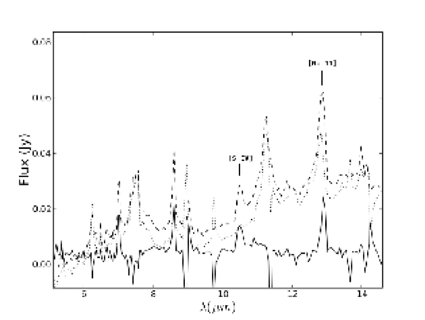
Figure 6.3: The short-wavelength, low-resolution spectrum of the PWN. Local background has been subtracted as described in the text. Dashed line is source $+$ background; dotted line is background; solid line is the spectrum of the source only.

For each of the SL orders, our procedure was as follows. First, we extracted spectra from three different, non-overlapping positions on each of the 5 slits. The positions corresponded to the middle and the ends of each slit. This gave us a total of 15 different spectra. Given the spatially varying background in the vicinity of the PWN, we elected to use only the background regions that were closest to the source. Thus, we excluded the 4 “corner” regions, leaving us with 11 total regions. We considered the middle 3 regions to be our “on-source” region (since flux from the PWN was extended into all 3) and added them together. We then used the remaining regions as background. As a check of this method, we integrated the background subtracted spectra over the appropriate wavelengths corresponding to the 5.8 and 8.0 $\mu$m IRAC channels, factoring in the spectral response curves. Within errors, we obtained the same flux here as we did using aperture photometry on the IRAC images. In Figure 6.3, we show the short-low spectrum of the PWN with the both the original source spectrum and background spectrum overlaid.

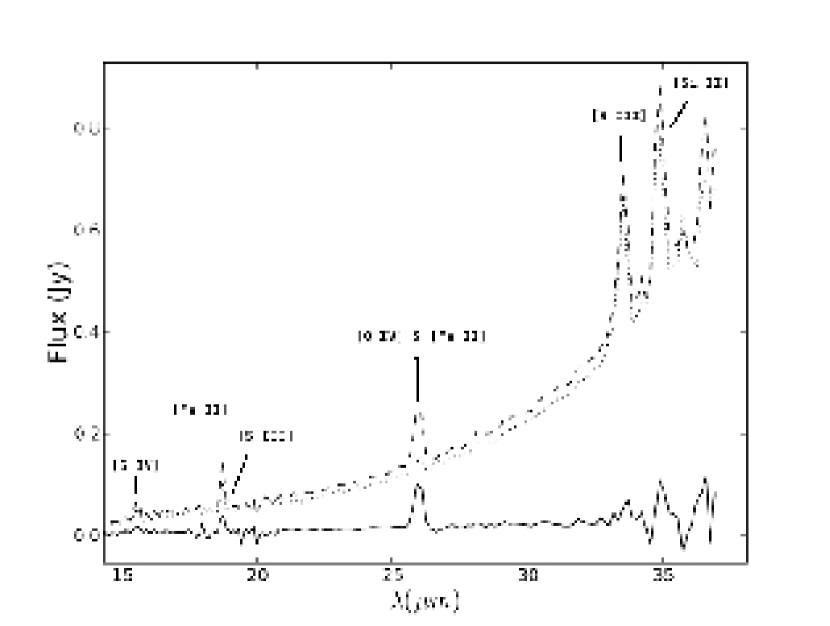
Figure 6.4: The long-wavelength, low-resolution spectrum of the PWN. Lines are the same as in Figure 6.3.

For the LL slits, we followed a similar procedure. Because we only had 3 parallel slit positions, we had 9 total spectra extracted from spatially different areas. Because the LL slit is wider than SL (about $10.5^{\prime\prime}$), we only considered the middle region of the middle slit to be the on-source region. In keeping with our policy of only using the closest background regions, we again excluded the 4 corner regions, and only used the 4 regions corresponding to the 2 middle regions of the parallel slit pointings, and the 2 extractions from the ends of the middle slit. We then averaged the 4 background spectra and subtracted the result from the on source spectrum to get a background subtracted spectrum. Again, as a check on this method, we integrated the resulting spectrum over the appropriate wavelengths, and with the appropriate spectral response curves, calculated a 24 $\mu$m flux that could be compared with that derived from aperture photometry on the MIPS image. Within errors, there was excellent agreement between these two methods. Figure 6.4 shows the long-low spectrum of the PWN.

In order to examine the shape of the synchrotron continuum from the low-resolution data, it was necessary to remove the lines from the spectra, as well as artifacts produced by obviously bad pixels. Although we detected the PWN at all wavelengths, the spatially varying background made our background subtraction procedure somewhat uncertain. Using different background subtraction regions does produce different results for the final spectrum, mainly due to the steep north-south gradient in the infrared background in the region of 0540 (see Figure 6.2). We believe our approach of defining an “annulus” region and averaging the backgrounds around the source is the best solution to this problem. However, it is not without significant uncertainties. We tried several variations of different background regions to see what the effects were. The largest differences came in comparing the two same-slit background positions with the two parallel slit background positions. We found variations in the absolute flux level between these two choices to be on the order of 40%. Because we have no reason to favor one over the other, we averaged them together with equal weights, thus creating our annulus. Because of this, we have used caution in interpreting the results of the extraction of the continuum. We also considered the possibility that a large number of weak lines could be interpreted as continuum. We reject this hypothesis for two reasons. First, there are only a handful of IR lines predicted in this wavelength range, and with the exception of [Ar III] at 8.99 $\mu$m, none of them even come close to the detection limit based on our line models. Second, we have high-resolution spectra of this region, and there is no evidence of lines that would be unresolved in the low-resolution data.

6.3.3 Line Fitting

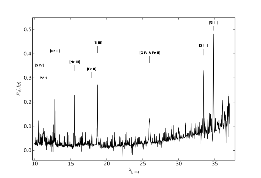
Figure 6.5: The high-resolution spectrum of the PWN, with no background subtraction. Measured lines are marked, along with a dust feature at ${\sim 11}\mu$m.

We used SPICE to extract spectra from the high-resolution data as well. In order to fit the lines, we used the open-source software Peak-O-Mat, which runs on SciPy (Scientific Python) and is available from http://lorentz.sourceforge.net/. Peak-O-Mat is an interactive program that is designed to fit curves using a least-squares algorithm to a user-specified function. Because our extraction region contains not only the entire expanding shell of the PWN, but also the foreground and background emission from the surrounding ISM, we expected to see both broad and narrow components for most of the lines detected, as has been seen in optical spectroscopy of the nebula. We assumed Gaussian profiles for both the broad and narrow components, and fit these on top of a linear background. We manually removed artifacts that were clearly caused by bad pixels, as determined by examining the 2-D dispersed image. We also clipped bad pixels from the backgrounds in the vicinity of each line, in order to make the fitting of the actual lines easier with a longer tail for the Gaussian. We did not remove or alter any of the pixels that were contained in the line itself, except in the case of the [Ne II] line at 12.8 $\mu$m. There was an obvious bad pixel that was contaminating the line structure at around 12.86 $\mu$m. In order to correct for this, we interpolated the strength of that pixel based on the strengths of neighboring wavelength pixels. Line profiles and strengths are discussed in section 6.4. The complete high-resolution spectrum of the PWN is shown in Figure 6.5.

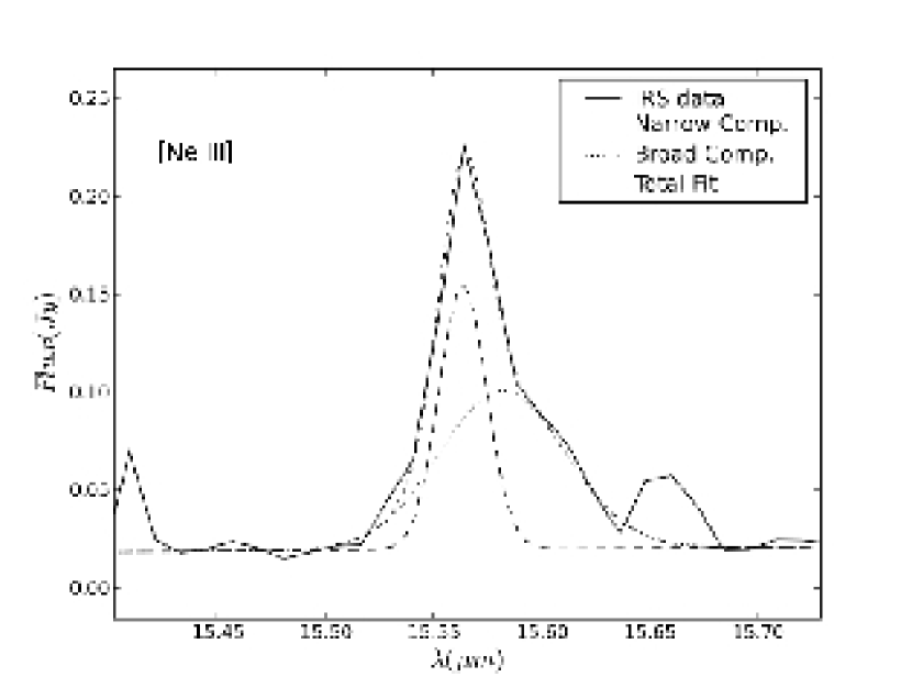
Figure 6.6: An example of our two-component fit to the lines identified in the high-resolution spectrum of the PWN. [Ne III] is clearly seen to have two components. Noisy pixels were clipped out for the fitting, but were left in this image to show their relative level of contribution.

We find that nearly all of the lines in the spectrum have a two-component nature, with a narrow component we attribute to the surrounding H II region, and a broad component coming from the PWN. Figure 6.6 shows an example of a two-component fit to a line, in this case [Ne III], at 15.5 $\mu$m. The spectral resolution of both SH and LH is $\lambda/\Delta\lambda$ $\sim 600$, which corresponds to a minimum FWHM of 500 km s^-1. Since we do not expect the narrow component widths to be wider than this, we fixed the narrow component widths to this value. Furthermore, the LMC has an overall recession velocity relative to the Sun of +270 km s^-1, so all narrow components should be redshifted by this amount. However, when we fixed the centroid of the Gaussian for the narrow component to this velocity, the fits were unacceptably poor. According to the Spitzer Observer’s Manual, the wavelength calibration in IRS is 1/5 of a resolution element, which for the high-resolution module corresponds to 0.003-0.011 $\mu$m, or 100 km s^-1. Since we found that all the narrow components seem to be off by a comparable systematic shift, we believe that the uncertainties in wavelength calibration are responsible. Thus, we measured the shift for each narrow component and averaged them to obtain a value to which we would fix each narrow component. We considered SH and LH separately, and calculated that each narrow component was redshifted on average (relative to its rest wavelength) 171 km s^-1 for SH and 230.5 km s^-1 for LH. Fixing the centroids of the narrow components to these values returned much more acceptable fits.

After we used Peak-O-Mat to determine the best values for the parameters of either one or two Gaussians, we then used our own least-squares algorithm to obtain errors. The errors listed on the parameters in Table 6.2 are 90% confidence limits, corresponding to a rise in $\chi^{2}$ of 2.706 from its minimum value. This procedure was repeated for each parameter separately. Errors on line fluxes were obtained through the standard error propagation formula.

6.4 Discussion

6.4.1 General Picture

We aim at a self-consistent, semi-quantitative picture of the PWN that accounts for the presence of lines (optical and IR), the extent of the synchrotron nebula, and the source of the [O III] emission at $8^{\prime\prime}$ radius. We find it useful to first point out some contrasts between 0540 and the most widely-known object of its class, the Crab Nebula. Although 0540 has been referred to as “The Crab’s Twin,” the two differ in some important ways. The most obvious difference is the lack of an outer shell in the Crab, while 0540’s $30^{\prime\prime}$ shell has been seen in both radio and X-ray observations. For the purposes of this paper, however, the important differences lie in the PWN. In the Crab, the size of the nebula decreases with increasing frequency, so that the radio nebula is larger than the optical, which is larger than the X-ray, etc. In 0540, the synchrotron nebula is approximately identical in extent throughout all wavelengths, around $5^{\prime\prime}$. The other fundamental difference is the presence in 0540 of emission located beyond the synchrotron nebula (the [O III] halo). There is nothing like this seen in the Crab, where the radio synchrotron emission extends to the outer boundary of anything known to be associated with the nebula.

In modeling the Crab Nebula, Sankrit & Hester (1997) considered two models, one a pure shock model and the other a pure photoionization model to explain the optical emission. They concluded that shocks from an expanding shell were more likely. In the case of 0540, however, a pure shock model cannot reproduce the [O III] extended emission. We therefore propose an extension to their models that incorporates both a global shock and photoionization. The specifics of our model will be described more fully in the sections below, but our general picture of the nebula is as follows. It is based on the dynamical picture of Chevalier (2005; C05).

Approximately a millenium ago, a star exploded via the core-collapse mechanism, leaving behind a pulsar, and sending a shock wave out into the interstellar medium. The outer boundary of this forward shock is now about 8 pc (angular distance of about $30^{\prime\prime}$) from the pulsar, and the reverse shock into the ejecta is somewhere between $10^{\prime\prime}-30^{\prime\prime}$, having not yet reached back to the inner ejecta. The pulsar has since formed a pulsar-wind nebula, which itself is driving a shock into the inner edge of the surrounding ejecta, which are in free expansion. The shock wave heats the inner ejecta and sweeps them into a thin shell. Since the shell of material is being continuously injected with energy from the pulsar, it is accelerating and overtaking less dense material as it expands. The shock speed relative to upstream material, however, reaches a maximum and then begins to drop since the free-expansion speed of the ejecta material is also higher at larger radii. There is no reason, however, to expect the ejecta to be completely homogeneous. The ⁵⁶Ni synthesized in the explosion will have heated the central ejecta by radioactive decay, causing them to expand in an “iron-nickel bubble” (Li, McCray, & Sunyaev, 1993), and compressing intermediate-mass ejecta into a denser surrounding shell.

We propose that the PWN shock has reached a radius of about 1.2 pc from the pulsar, which corresponds to a size of $\sim 5^{\prime\prime}$, the size of the nebula as determined by X-ray observations. The layer of shocked ejecta is geometrically thin, bounded on the inside by a contact discontinuity separating it from the the PWN proper, which is the shocked pulsar wind. The shock has already encountered and propagated through the low-density iron-nickel bubble and its surrounding shell. That shell is likely to be highly clumpy (Basko, 1994); shocks driven into the clumps of heavy-element ejecta will be slow. Finally, at a sub-arcsecond radius we expect the inward-facing pulsar wind shock where the relativistic pulsar wind is thermalized. Interior to the shock driven into the ejecta, emission in optical/IR is both thermal and non-thermal, with the dominant component being synchrotron continuum emission from the relativistic electrons. However, multiple emission lines are clearly detected from dense clumps and filaments of thermal gas. In addition to this, we identify a rising continuum in the mid-infrared above the synchrotron continuum that we interpret as a small amount of warm dust, collisionally heated by electrons heated by the shock. Most lines seen in optical and infrared then come from dense clumps of ejecta, where the shock wave has slowed significantly and become highly radiative.

What remains is to explain the faint [O III] emission seen at $8^{\prime\prime}$. We propose that this is material that is still in free expansion, i.e. unshocked, that has been photoionized by ultraviolet photons emitted from the shockwave. The source of photoionization is two-fold; ultraviolet photons from the synchrotron nebula and those produced in fast radiative shocks both contribute appreciable amounts of ionizing radiation. We show below that to within a factor of 2, there are enough ionizing photons produced to account for the [O III] halo at $8^{\prime\prime}$.

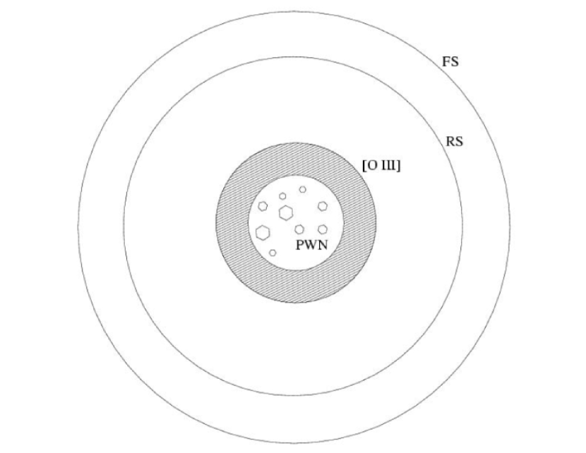
Figure 6.7: A cartoon sketch of our general picture discussed in section 4.1. Not to scale. FS refers to the forward shock from the SN blast wave, at a radius of $\sim 30^{\prime\prime}$. RS refers to the reverse shock, which has not yet been observed, and is at an unknown position between 10 and 30^′′ from the pulsar. [O III] refers to the extent of the halo of material that has been photoionized, and is seen in optical images to extend to 8^′′. PWN refers to the edge of the shock driven by the pulsar wind, and is located at a radius of 5^′′. Interior to this shock, ejecta material has fragmented into clumps. The PWN as a whole is observed to have a redshifted velocity as reported in previous optical observations, possibly resulting from a pulsar kick. This is also the region where relativistic particles from the pulsar create observed synchrotron emission; see discussion in text.

We have included, in Figure 6.7, a cartoon sketch of this picture, which will be further discussed in the following sections. A factor of a few is all we expect to be able to accomplish in modeling the nebula, due to the large uncertainties involved. These uncertainties include, but are not limited to; nature of the progenitor star (which affects the post-explosion density distribution of the ejecta), heavy element abundances in the ejecta, degree of clumping of the ejecta, etc. We have endeavored in the following sections to point out places where uncertainties arise, and where possible, to assign quantitative values to them.

6.4.1.1 PWN Model

C05 discusses a model, based on a thin-shell approximation, for a pulsar wind nebula interacting with an inner supernova ejecta density profile. We have used this model along with our observations to determine various quantities about 0540, including how much hot gas should be present. Observable quantities for the pulsar include period ($P$), period derivative ($\dot{P}$), luminosity ($\dot{E}$) and for the nebula, size ($R$) and shell velocity ($V_{sh}$). While the quantities for the pulsar are fairly well established by previous observations, those for the PWN are much more uncertain. Previous optical studies of the remnant (Mathewson et al., 1980; Kirshner et al., 1989), as well as radio observations (Dickel et al., 2002) interpreted the PWN as a bubble of radius $\sim 4^{\prime\prime}$, and the optical observations gave expansion velocities less than 1400 km s^-1. Based on Chandra observations, Petre et al. (2007) concluded the nebula was slightly larger, with a radius of $\sim 5^{\prime\prime}$. We shall adopt $5^{\prime\prime}$ (1.2 pc) as an estimate of the location of the ejecta shock.

However, Morse et al. (2006) detected faint [O III] emission in images extending out to a radius of $\sim 8^{\prime\prime}$. Based on similarities to the Crab Nebula, they interpreted this [O III] halo as being the outer edge of the shock from the pulsar wind overtaking the slower moving ejecta. Here we present an alternative interpretation of this [O III] halo emission. We propose that it is undecelerated ejecta that have been photoionized, rather than shock-ionized. The FWZI of the [O III] emission from Morse et al. was 3300 km s^-1, which, given the extent of 1.8 pc and our interpretation of this as undecelerated ejecta, provides the remnant age of 1140 years. While this is somewhat longer than the favored model of Reynolds (1985), it is at least reasonable given other age estimates made by previous studies of the object. Photoionization calculations are discussed in Appendix B.

As a first attempt to model the observations, we considered the case of a spherically symmetric shock wave driven by the energy input from the pulsar expanding into a medium with density profile described by $\rho_{SN}=At^{-3}(r/t)^{-m}$. We considered different values of the parameter $m$, as dynamical mixing between the ejecta and surrounding medium would produce a complicated density structure. The swept-up mass does not exceed $1M_{\odot}$ in this model. Although this model did a reasonably good job at producing shock speeds high enough to account for the necessary dust grain heating rate, a spherically symmetric model does not adequately reproduce line radiation observed in both optical and IR. A slow shock into dense material is required to explain these lines, and the spherical model cannot account for this, since presence of lines requires a departure from the overall homogeneous density profile. We present the spherically symmetric calculations in Appendix C. A more robust model is required to explain both the slow shocks required for lines and the faster shocks required for dust emission. We will return to this picture at the end of the following section, but we must first describe our line observations in detail.

6.4.2 Lines

Eight emission lines are detected in the Spitzer spectrum. They provide constraints on the density and temperature of the emitting gas, and perhaps more importantly on the elemental abundances. They complement the optical spectra published by Kirshner et al. (1989) (K89), Morse et al. (2006) (M06) and Serafimovich et al (2005) (S05). We first summarize the implications of the optical spectra, then consider shock wave models for the combined optical and IR emission.

Several temperature estimates are available from the optical spectra. The [O III] line ratio I(4363)/I(5007) gives temperatures of about 24,000 K according to S05 or 34,000 K (K89). According to the CHIANTI database (Landi et al., 2006), the ratio given by K89 corresponds to 50,000 K, while that given in M06 implies 24,000 K. K89 also find temperatures $>$30,000 K from the [O II] I(7325)/I(3727) ratio and $<$10,000 K from [S II] I(4072)/I(6723). The [S II] ratio of M06 implies $T$ = 14,000 K. Assuming a temperature of 10,000 K, S05 find a density of 1400 – 4300 $\rm cm^{-3}$, and at 14,000 K the range would be 1700 – 5000 $\rm cm^{-3}$. The differences among the various temperature estimates may result partly from different reddening corrections and different slit positions, but it is clear that the [O III] lines are formed in hotter gas than the [S II] lines. The Spitzer data include only one pair of lines from a single ion, [Fe II] I(17.9$\mu$)/I(26.0$\mu$), which is constrained to be larger than 1.13. Again using CHIANTI, this requires a density above about 5000 $\rm cm^{-3}$ and a temperature above 4000 K. However, the ratio depends upon the deblending of the [Fe II] and [O IV] lines at 26$\mu$m, and the uncertainty may be larger than the formal value. The density contrast between the optically emitting material and the mean post-shock density from the global model indicates that as in the Crab Nebula, optically emitting material is concentrated in dense knots and/or filaments.

The next step in interpreting the spectra and constructing models is to estimate the relative importance of photoionization and shock heating. In the Crab nebula, photoionization dominates, though shocks are important for the UV lines produced at higher temperatures and for compressing the gas to increase the optical emissivity (Sankrit & Hester, 1997). In the oxygen-rich SNRs, such as N132D and 1E0102-7219, shock heating dominates (Blair et al., 2000). 0540 shows both synchrotron emission reminiscent of the Crab and extreme heavy element enhancement. A pure photoionization model with strongly enhanced abundances and the observed density gives too low a temperature to account for the [O II], [O III] and [S II] line ratios, while shock models cool so rapidly that they produce little [O I] or [S II] unless they produce no [O III] at all. Therefore, it seems likely that a model of a shock including the PWN ionizing radiation is needed.

We have computed models with the shock model described in Blair et al. (2000) illuminated by the power law continuum described by Serafimovich et al. (2004). Briefly, the code is similar to that of Raymond (1979) and Cox & Raymond (1985), but it has been modified to describe SNR ejecta with little or no hydrogen. The most important difference is that the cooling rate is enormous, so that the electron temperature is well below the ion temperature in the hotter parts of the flow. The model is similar to those of Itoh (1981) and Sutherland & Dopita (1995). Unlike those models, we do not include the photoionization precursor of the shock, because the ionizing emission from the shock is considerably weaker than the ambient synchrotron radiation. In comparison with the spectra of Cas A, N123D and 1E0102-7219, shock models have the problems that no single shock model produces the observed range of ionization states, and that they tend to predict too much emission in the O I 7774 Å recombination line unless the cooling region is somewhat arbitrarily truncated (Itoh 1988). However, they do predict reasonable relative intensities from the UV to the near IR for O III and O II. Below, we attribute the truncation to mixing with hotter, lower density gas.

We assume a 20 $\rm km~{}s^{-1}$ shock with a pre-shock density of 30 $\rm cm^{-3}$, which produces a density of around 5000 $\rm cm^{-3}$ where the [S II] lines are formed. The elemental abundances are O: Ne: Mg: Si: S: Ar: Ca: Fe = 1: 0.2: 0.1: 0.1: 0.1: 0.1: 0.1: 0.1 by number. H, He and N are not included in the model, because it seems likely that the lines from these elements arise in some other gas, like either the quasi-stationary flocculi or the outer shell of ejecta seen as very fast knots in Cas A (Kirshner & Chevalier, 1977; Fesen, 2001). The normalization of the power law flux assumes that the shocked gas is 1 pc from the center of the PWN.

The list of caveats is long. There is undoubtedly a range of shock speeds and pre-shock densities. The shocked gas is unlikely to be a uniform mixture of the various elements, and large variations in the composition among different clumps, as observed in Cas A, are likely. There may well be a significant contribution from unshocked photoionized gas for some lines (e.g., Blair et al., 1989), as we shall argue below for the [O III] halo. The shock models are plane parallel, with the power law illumination incident from the PWN, while the X-rays are more likely to illuminate the shocked gas from behind. The models terminate somewhat arbitrarily at 250 K because of numerical limitations. This will affect the IR lines and the O I recombination line at 7774 Å. Also, as a compromise between energy resolution and energy range of the ionizing radiation, the power law only extends to 2 keV. This means that the inner shell ionization and Auger ionization of S and Fe is not included. Finally, the atomic data in the code are somewhat out of date and need to be updated. Nevertheless, the code gives a reasonable idea of the relative line intensities.

To compare this model with our observed IR spectra, we must place the Spitzer spectrum on the same scale as the optical spectra. We normalize the IR lines to [O III] 5007 = 100 by dividing the Spitzer intensities by 4 times the [O III] 5007 intensity given by M06. The factor of 4 is meant to account for the fact that the $2^{\prime\prime}$ slit used by M06 covers only about 1/4 of the remnant. This is obviously not a very accurate correction, but it is probably good to a factor of 2. Since the relative fluxes of many optical lines differ by a factor of 2 between M06 and K89, this is unfortunately the best we can do until an optical spectrum of the entire remnant becomes available.

The result is shown in Table 3. Overall, the agreement is astonishingly good for such a simple model. Several of the low ionization lines, [O I], [Ne II] and [Si II] are underpredicted, though the [Si II] line could be increased simply by increasing the silicon abundance. The ratio of the [S IV] to [S III] IR lines is too low, but inclusion of the harder part of the power law spectrum would improve that. Inclusion of the harder X-rays would also increase the intensity of the [Fe VII] line, though a lower pre-shock density or a higher shock speed would have the same effect. The oxygen column density of the model is only about $10^{14}~{}\rm cm^{-2}$, and the thickness of the emitting region is only $6\times 10^{11}$ cm. If the thickness were large enough to allow the remaining O⁺ to recombine, the predicted O I recombination line, which is comfortably lower than the weakest detected lines, would increase to about 4 times the apparent detection limit of K89. The agreement would improve if the argon abundance were cut in half, but otherwise the abundances appear to match the observations.

The shock model shown in Table 2 produces $1.1\times 10^{-14}~{}\rm erg~{}cm^{-2}~{}s^{-1}$ in the [Ne III] 15.5 micron emission line, so the flux shown in Table 1 would come from a region with surface area of $2\times 10^{38}$ cm². This area is roughly equal to the area of a sphere of $5^{\prime\prime}$ radius but the emission could come from many smaller volumes with a total filling fraction of a few percent. Heavy-element ejecta enter these slow shocks at a rate of $\sim 0.01M_{\odot}$ yr^-1.

We conclude that, as in the Crab (Sankrit & Hester, 1997), the observations can be explained by shocks that heat and compress the gas in the radiation field of the PWN. The shock heating seems needed to reach the high temperatures seen in some line ratios and to provide the high densities observed, while the photoionization heating strengthens the low and moderate ionization lines. Oxygen is about ten times as abundant as the other elements. The shock speed and pre-shock density are not very well constrained, but a shock as fast as 80 $\rm km~{}s^{-1}$ requires a low pre-shock density to match the observed density, and that in turn implies a very high pre-shock ionization state, overly strong [O IV] and overly weak [O II] emission.

In the last 100 years alone, about 1 $M_{\odot}$ of heavy-element ejecta have been shocked, more than the total mass of the swept-up ejecta in the global model described in Appendix B. This casts some doubt on the validity of the global, spherically symmetric model, where density within freely expanding ejecta was assumed to be a smooth power-law. It is possible that the innermost ejecta have been swept-up by an iron-nickel bubble, as inferred for SN 1987A by Li, McCray, & Sunyaev (1993) and modeled by Basko (1994) and Wang (2005) (see also brief discussion in C05). We explored the possibility that the global shock could be contained within the shell swept-up by the iron-nickel bubble. In this one-dimensional picture, the shock passed through the inner, low-density region in $\sim 50$ years, and has since been contained within the high-density ($n\sim 30$ cm^-3) bubble wall. We varied parameters of the model until the shock speed in the bubble was approximately 20 km s^-1, as required by line models. We find, however, that the mass flux of material entering the shock throughout the remnant’s entire lifetime has been unreasonably high for this model, approximately $0.01(t/1140$ yr$)^{-1/2}M_{\odot}$ yr^-1. In addition, a 20 km s^-1 shock, even at such density, would not adequately heat dust grains to temperatures observed. Dust heating is discussed in more detail in section 6.4.3.3.

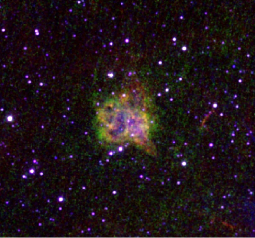
Figure 6.8: Hubble Space Telescope WFPC2 image of PWN 0540-69.3, from Morse et al. (2006). Colors are: Blue - F791W continuum; Green - F502N [O III]; Red - F673N [S II]

We are forced to consider inhomogeneous ejecta with a fast global shock to heat dust to observed temperatures, and slower shocks producing observed line emission. We propose the following picture: The shock swept through the low-density iron-nickel bubble interior early in the life of the SNR. It then encountered the dense, clumpy shell of the bubble, slowing down and further fragmenting the shell into dense clumps, which are still being overrun by slow shocks, currently 20 km s^-1. The global shock has now exited the iron-nickel bubble shell, and is propagating through the ejecta with relatively low ambient density. The speed of this shock is not well known, but 250 km s^-1 would be sufficient to heat the dust to the observed temperature of around 50 K (see below). Assuming pressure equilibrium between the dense clumps and the ambient ejecta, we derive a density contrast, given the difference in shock velocities, of $\sim 150$. Support for this model can be inferred from HST images of the nebula, as seen in Figure 6.8, which shows [O III] filaments in the interior, not just in a shell. [O III] line profiles (M06) also do not match the shape that would be expected from a spherically symmetric expanding shell, i.e. a flat top. The slow shocks driven into the dense clumps are in rough pressure equilibrium with the fast shock driven into the less dense ejecta.

6.4.2.1 Progenitor Mass

We have compared the abundances of heavy elements listed in section 6.4.2 with the predicted abundances of Woosley & Weaver (1995), who consider abundance yields from core-collapse SNe ranging in mass from 11-40 $M_{\odot}$ and metallicities between zero and solar. We consider models with both solar and 0.1 solar metallicity, as this range is most likely to reflect a massive star in the LMC. Our abundances listed are somewhat uncertain, and result from fits to optical and infrared line strengths. We considered the ratios of O to Ne, Mg, Si, and Fe. The data do not single out a particular model from Woosley & Weaver (1995), but ratios of heavy elements to oxygen do favor a low-to-medium-mass progenitor. High-mass progenitors ($\mathrel{\mathchoice{\lower 3.1pt\vbox{\halign{$\m@th\displaystyle\hfil#\hfil$\cr>\crcr\sim\crcr}}}{\lower 3.1pt\vbox{\halign{$\m@th\textstyle\hfil#\hfil$\cr>\crcr\sim\crcr}}}{\lower 3.1pt\vbox{\halign{$\m@th\scriptstyle\hfil#\hfil$\cr>\crcr\sim\crcr}}}{\lower 3.1pt\vbox{\halign{$\m@th\scriptscriptstyle\hfil#\hfil$\cr>\crcr\sim\crcr}}}}$ 30 $M_{\odot}$) are less favored, since they produce larger amounts of oxygen relative to other elements. This interpretation is consistent with that of Chevalier (2006), who favored a type IIP explosion for this object based on observations of hydrogen in the spectrum. This is also consistent with the idea that type IIP SNe should result from the explosion of a single star of 8-25 $M_{\odot}$ (Woosley et al., 2002).

It is possible to quantify these results even further. If we assume a constant heavy-element mass flux through the radiative shocks for $10^{3}$ yr of 0.01 $M_{\odot}$ yr^-1 with our abundances listed above, we get a total ejected mass in oxygen of $\sim 3.5M_{\odot}$, though this number should only be considered accurate to a factor of a few, and is likely an upper limit. When compared with predictions from models, this value favors stars in the range of 20-25 $M_{\odot}$. Maeder (1992) gives slightly different abundance yields for SNe, with lower overall oxygen abundances produced. In his model, high-mass stars ($\mathrel{\mathchoice{\lower 3.1pt\vbox{\halign{$\m@th\displaystyle\hfil#\hfil$\cr>\crcr\sim\crcr}}}{\lower 3.1pt\vbox{\halign{$\m@th\textstyle\hfil#\hfil$\cr>\crcr\sim\crcr}}}{\lower 3.1pt\vbox{\halign{$\m@th\scriptstyle\hfil#\hfil$\cr>\crcr\sim\crcr}}}{\lower 3.1pt\vbox{\halign{$\m@th\scriptscriptstyle\hfil#\hfil$\cr>\crcr\sim\crcr}}}}25M_{\odot}$) actually produce less oxygen than their lower-mass counterparts, due to mass-loss of outer layers and inability to synthesize O from He and C. However, these massive stars would be Wolf-Rayet stars, and can be ruled out based on the detection of hydrogen in optical spectra.

6.4.3 Dust

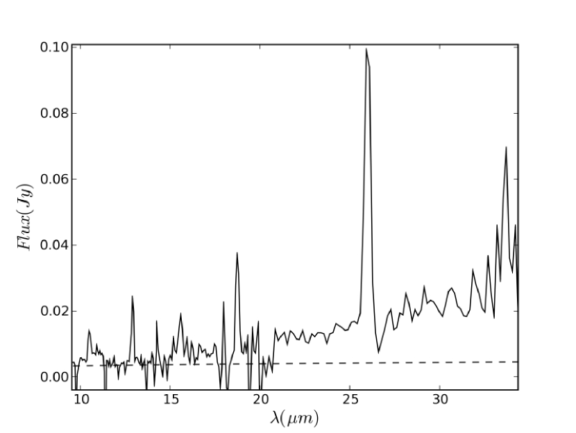
Figure 6.9: The background-subtracted low-resolution spectrum of the PWN is plotted as the solid line, with the radio synchrotron component shown as a dashed line. A clear rising excess can be seen longward of 20 $\mu$m.

One of the more obvious features of the continuum in 0540 as seen in Figure 6.9 is the excess of emission above the extrapolated radio synchrotron spectrum at longer wavelengths. A similar excess has been observed in the Crab (Temim et al., 2006), and has been attributed to warm dust. We have inferred the temperature and the amount of dust present, and have examined several possible mechanisms for grain heating.

In order to fit the long-wavelength excess above the continuum, it was necessary to remove contributions from emission lines and the underlying synchrotron continuum. The flux contributed by the lines is negligible, but their presence makes fitting of a model dust spectrum more difficult. We have thus clipped obvious emission lines and bad pixels out of the spectrum for this analysis.

6.4.3.1 Synchrotron Component

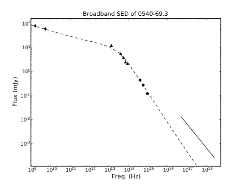
Figure 6.10: Broadband spectrum of 0540. Radio points (diamonds): Manchester et al. (1993). IR points (triangles): our MIPS and IRAC fluxes. Optical points (circles): Serafimovich et al.  (2004). X-rays (solid line): Chandra (Kaaret et al. 2001). Dashed line: model described in text.

In order to subtract the synchrotron component, it was necessary to produce a model synchrotron spectrum that includes the break in power-law indices from optical to radio. The synchrotron model used here is one of a class of simple outflow models in which various quantities are allowed to have power-law dependencies on radius: flow-tube width, flow velocity, gas density (where mass loading might allow a range of possibilities), and magnetic-field strength (Reynolds, in preparation). Such models can produce synchrotron-loss steepening in spectral index both steeper and flatter than the homogeneous-source value 0.5 (Reynolds, 2006). Here the model, used for illustrative purposes, invokes a simple outflow geometry with conical flow tubes (width $w\propto r$), mass increasing as radius (due presumably to mass loading), flow velocity decreasing as $r^{-2}$ roughly, and magnetic field as $r^{-1}$. The initial magnetic field at the injection radius is $B_{0}=2.5\times 10^{-4}$ G. This model predicts a decrease in size with frequency as $\theta\propto\nu^{-0.34}$, which might be slow enough to be consistent with observations, especially as it might take place along the line of sight. While this is not meant as a definitive model for 0540, it describes the data well as shown on Figure 6.10 and was used to estimate the synchrotron contribution.

The result of radiative losses on electrons above the break energy in a flat ($N(E)\propto E^{-s}$ with $s<2$) energy distribution is for such electrons to move to just below the break energy, where they can produce a perceptible “bump”. However, the “bump” is almost undetectable unless $s$ is very close to 0; for the 0540 value $s=1.5$, there is almost no departure from the power-law below the break frequency. The model in Figure 6.10 was calculated including the redistribution of electron energies, and it can be seen that the excess we observe below 24 $\mu$m cannot be attributed to this cause.

6.4.3.2 Fitting the Dust Component

This left us with a residual rising continuum that we then fit with a model dust spectrum. Since we presume that the dust present in 0540 would be newly formed ejecta dust, as seen in SN 1987A (Ercolano et al., 2007), we have little a priori knowledge about the grain-size distribution. However, since the wavelength of IR radiation is much larger than typical ISM grain sizes, we adopt a model with a single grain size, arbitrarily chosen to be $a=0.05$ $\mu$m in radius. In any case, in the limit of $a$ $\ll\lambda$, the results are independent of the choice of grain radius. We also do not know the grain composition, as general results from the LMC should not apply to ejecta dust. We thus consider two models; a graphite dust model and the “astronomical silicates” model of Draine & Lee (1984). We calculate the dust grain absorption cross section for both as a function of wavelength. We then fit a simple modified blackbody model (incorporating the grain absorption cross-section) to the data using a least-squares algorithm designed for this model. We obtain a dust mass of $\sim 3\times 10^{-3}$ $M_{\odot}$ at a temperature of $50\pm 8$ K for silicate dust, while the resulting fit to the temperature with graphite grains was slightly higher, $\sim 65$ K, and the required dust mass was lower, $\sim 1\times 10^{-3}$.

The errors on the dust temperature are estimates based on using different methods of removing lines and subtracting the background and the underlying synchrotron spectrum. The resultant dust spectrum is sensitive to these details. The dust mass should be considered uncertain, and is probably only accurate to within a factor of a few, as evidenced by the difference between derived masses for graphite and silicate grains. Our data do not allow us to distinguish between various dust compositions. It should also be noted that we are only sensitive to dust that has been warmed by the shock wave from the pulsar wind, and that there could be more dust that has not yet been shocked, and is still too cool to be detected. Thus, our mass estimate should be considered a lower limit.

6.4.3.3 Grain Heating Mechanisms

We now turn our attention to heating mechanisms for this dust. We first consider heating by the synchrotron radiation field from the PWN. Since the spectrum of the synchrotron radiation is known in the optical/UV portion of the spectrum and grain absorption cross-sections can be calculated as a function of wavelength, it is possible to estimate whether there is enough radiation to heat the dust to temperatures observed. We calculate the optical depth of the dust around the PWN, and integrate over all wavelengths from radio up 1 keV. Although the flux from the PWN is higher at longer wavelengths, most of the absorption occurs in the optical/UV portion of the spectrum, due to the steeply rising absorption cross-sections in this regime. We compare this number to the luminosity in dust derived from our dust model, $\sim 5\times 10^{35}$ ergs s^-1. A simple calculation showed that the radiation available falls short by several orders of magnitude of what is necessary.

However, this method tells us nothing about the total amount of dust that could be present to absorb the synchrotron radiation. Thus, to further test this hypothesis, we calculated the temperature to which dust would be heated if it were exposed to such an ultraviolet radiation field. We find that dust would only be heated to $\sim{20}$ K. If this were the source of the emission seen in IRS, it would predict a 70 $\mu$m flux that is several orders of magnitude higher than the upper limit we have placed on emission there. Given that these order of magnitude estimates are drastically inconsistent with our observations, we consider heating by photons from the PWN to be ruled out.

We then considered the somewhat more exotic possibility of the observed excess arising from a protoplanetary disk around the pulsar, unassociated with the nebula. It has long been known that planets can form around pulsars (Wolszczan & Frail, 1992), and the supposition has been that these planets arise from a protoplanetary disk around the pulsar, the source of which has been attributed to several mechnisms (Bryden et al., 2006). Various surveys of known pulsars have been made in infrared and submillimeter wavelengths, but for the most part these surveys have only produced upper limits on the dust emission present.

However, Wang et al. (2006) conducted a survey of neutron stars with IRAC and found a debris disk around the young isolated neutron star 4U 0142+61. The authors suggest that the age of the debris disk compared to the spin-down age of the pulsar favors a supernova fallback origin. The IRAC observations combined with K-band Keck-I observations suggest a multi-temperature thermal model with temperatures ranging from 700-1200 K, where the disk has inner and outer radii of 2.9 and 9.7 $R_{\odot}$, respectively. Using the same model the authors use (Vrtilek et al., 1990), we calculate the necessary radius to reproduce observed fluxes for 0540 for a disk with temperature $\sim{50}$ K to be on the order of $10^{4}$ $R_{\odot}$. A survey of disks around Anomalous X-ray Pulsars (AXPs) (Durant & van Kerkwijk, 2005) found several candidates for fallback disks which consistently had IR(K-band)/X-ray flux ratios of order $10^{-4}$. Although we were not able to find any archival near-infrared observations of the PWN, we can make an estimate of this ratio by looking at the overall spectrum of the IRAC and optical points. An estimate of $5\times 10^{-2}$ is reasonable for this ratio in 0540, significantly different than that found in the AXPs. Additionally, Wang et al. (2007) observed 3 known AXPs with Spitzer, and found no mid-IR counterpart to any of them. Given these discrepancies between these cases and that of 0540, we do not believe that a protoplanetary disk around the pulsar is the origin of the far-IR excess.

What then is the cause? Collisional heating by hot gas heated by shocks driven into the ejecta can provide both a qualitative and quantitative explanation for the dust present. Grain heating rate, $\cal{H}$, goes as

$$\mathcal{H}\propto n_{e}v_{e}T_{e}\propto PT_{e}^{1/2},$$ (21)

where $n_{e}$, $v_{e}$, and $T_{e}$ are electron density, velocity, and temperature, and $P$ is the pressure, $nT$. In the PWN, P is constant throughout the bubble, so that grain heating is more efficient in hotter gas. We find that the slow, radiative shocks are incapable of heating dust grains to temperatures much above $\sim 25$ K. Faster shocks, and thus higher temperatures, are required to heat grains to observed temperatures.

To determine whether this is plausible, given the conditions in the object, it is necessary to make an estimate of the amount of gas that is still hot, i.e. capable of heating dust grains through collisions with electrons. The shock cooling time (McKee, 1987) is

$$t_{cool}=2.5\times 10^{10}v^{3}_{s7}/\alpha\rho_{0},$$ (22)

where $v_{s7}$ is the shock speed in units of $10^{7}$ cm s^-1, $\rho_{0}$ is the pre-shock density in amu cm^-3, and $\alpha\geq 1$ is a parameter for the enhancement of cooling due to higher metal content. We find that a shock with velocity $\sim 250$ km s^-1 would effectively heat dust to 50 K, with a pre-shock density of $\sim 8$ amu cm^-3, assuming the same pressure as in slow shocks. If the dust component is composed of graphite grains at $\sim 65$ K, a slightly faster shock of 325 km s^-1 is required. Using the above equation, we find that the amount of hot gas is on the order of a few tenths of a solar mass. This yields dust-to-gas ratios of a few percent. Given the unknown dust content within the inner ejecta of a supernova, we believe this is a reasonable explanation.

As a check on the constraints of such a fast shock, we calculated the expected X-ray emission from such a shock, and found it to be below the upper limits of thermal X-ray emission observed from the PWN, except for very metal-rich ejecta.

6.4.4 Origin of O-rich Clumps

Matzner & McKee (1999) considered a spherically-symmetric explosion of a 15 $M_{\odot}$ RSG, and found that its He core and heavy element ejecta formed an approximately constant density, freely expanding ejecta core. C05 rescaled their results to other values of ejecta mass $M_{ej}$ and kinetic energy $E_{51}$, arriving at the core density of

$$\rho_{c}t^{3}=2.4\times 10^{9}(M_{ej}/15M_{\odot})^{5/2}E_{51}^{-3/2}{\rm g\ cm^{-3}\ s^{3}}.$$ (23)

An additional compression is expected from the iron-nickel bubble effect. For the centrally-located Ni with mass $M_{Ni}$, the adjacent ejecta are expected to be swept up into a shell with velocity

$$V_{1}=975(M_{Ni}/0.1M_{\odot})^{1/5}(\rho_{c}t^{3}/10^{9}{\rm g\ cm}^{-3}\ {\rm s}^{3})^{-1/5}{\rm km\ s^{-1}}.$$ (24)

The compression within the Fe-Ni bubble shell is at least by a factor of 7, expected in strong, radiation dominated shocks with $\gamma=4/3$. The shell density increases inward from a shock front to a contact discontinuity separating the shocked ejecta from the Fe-Ni bubble. In one dimensional hydrodynamical simulations, Wang (2005) finds an average shell compression by a factor of 20. The average shell density is then

$$\rho_{1}t^{3}=4.8\times 10^{10}(M_{ej}/15M_{\odot})^{5/2}E_{51}^{-3/2}{\rm g\ cm^{-3}\ s^{3}}.$$ (25)

(Diffusion of radiation might reduce this compression by a modest factor of $\leq 2$ – Wang 2005.) At the current remnant’s age of 1140 yr, the shell density is

$$\rho_{1}=1.0\times 10^{-21}(M_{ej}/15M_{\odot})^{5/2}E_{51}^{-3/2}{\rm g\ cm^{-3}}.$$ (26)

Because the dense iron-nickel bubble shell has been accelerated by low-density gas within the bubble, the shell is subjected to the Rayleigh-Taylor instability, and we expect it to fragment into clumps. Within a factor of 2, their expected density is equal to the preshock density for the O-rich clumps in 0540. We conclude that these clumps are remnants of the iron-nickel bubble shell.

Matzner & McKee (1999) found a sharp density drop by a factor of 10 at the interface between the He core and the H envelope, with an approximately constant density through much of the H envelope. The envelope density $\rho_{env}$ is then

$$\rho_{env}t^{3}=2.4\times 10^{8}(M_{ej}/15M_{\odot})^{5/2}E_{51}^{-3/2}{\rm g\ cm^{-3}\ s^{3}},$$ (27)

200 times less dense than the iron-nickel bubble shell. This density contrast is similar to the density contrast inferred between the O-rich clumps and the more tenuous inter-clump gas. It is likely that the PWN nebula expands now into the H envelope. Because the dense He core has been decelerated by the less dense H envelope during the SN explosion, the ensuing Rayleigh-Taylor instability led to a large-scale macroscopic mixing between them. As a result, we expect a two-phase medium ahead of the PWN shell, consisting of more tenuous H-rich gas and denser He-rich gas. It is possible that shocks driven into the He-rich gas became radiative; that could explain the presence of H and He recombination lines in optical spectra of 0540.

The dense iron-nickel bubble shell should contain not only O-rich ejecta, substantial amounts of He-rich gas are also expected. Slow (20 km s^-1) shocks driven into the dense He-rich gas may also become radiative; if so, they could produce strong lines of low ionization species. This could explain excess emission seen in optical and IR spectra for low ionization species (see discussion in § 4.2). More detailed shock models are necessary to determine whether or not our picture is consistent with observations.

The identification of dense O-rich clumps in 0540 with a compressed and fragmented shell swept up by the iron-nickel bubble has important implications for ejecta detection in SNRs. Dense O-rich clumps are expected to produce strong optical or X-ray emission, once shocked and heated by the reverse shock. The optical emission should be most prominent for remnants with a particularly dense ambient medium, either of circumstellar (e.g., Cas A) or interstellar (N132D) origin. The entire class of optically emitting O-rich remnants may owe its existence to the iron-nickel bubble effect. For ejecta expanding into less dense ambient medium, X-ray emission is expected instead since clumps will be reverse-shocked much later when their densities dropped significantly because of free expansion. The O-rich clumps such as seen in 0540, even when shocked to X-ray emitting temperatures 10,000 yr after the explosion, will have substantial ($\sim 1$ cm^-3) electron densities and emission measures. Even old remnants should show O-rich ejecta in their interiors, in agreement with the accumulating evidence gathered by modern X-ray satellites. A good example is a 14,000 yr old SNR 0049 $-$73.6 in the SMC, where Chandra imaging and spectroscopy revealed the presence of a clumpy O-rich ring in its interior (Hendrick, Reynolds, & Borkowski, 2005). Hendrick et al. interpreted this ring as the shell swept up by the iron-nickel bubble, based on mostly theoretical arguments. Observational evidence for the iron-nickel bubble effect in 0540 strengthens this interpretation for 0049$-$73.6, and possibly for many more mature SNRs with detected ejecta emission in their interiors.

Dust formation is most likely to occur where ejecta density is the highest. The dense O-rich clumps likely contain dust; this dust may survive the passage through the radiative shock. If it were mixed into the much hotter ambient medium, this surviving dust may be the source of the observed infrared emission.

6.5 Summary

We have observed the supernova remnant B0540-69.3 with all three instruments aboard the Spitzer Space Telescope. We detected the PWN in all 4 IRAC bands, as well as the 24 $\mu$m MIPS band. We did not detect any emission from the PWN at 70 $\mu$m, though the upper limit is rather unconstraining. We found no hint of detection at any wavelength of the $\sim 30^{\prime\prime}$ shell surrounding the PWN, as seen in X-rays and radio. Both the IRAC and the MIPS 24 $\mu$m photometric fluxes are consistent with the emission being primarily dominated by synchrotron emission, as synchrotron models extended both down from the radio and up from optical wavelengths roughly reproduce the flux seen in infrared. There is a change in slope of the overall synchrotron spectrum taking place in mid-infrared wavelengths, as is required to match the radio synchrotron power-law with the optical power-law.

The IRS spectra in the 10-37 $\mu$m region show a clear excess of infrared emission that cannot reasonably be attributed to any synchrotron radiation. We conclude that this excess emission is coming from a small amount ($\sim 1-3\times 10^{-3}M_{\odot}$) of warm dust that has been formed in the expanding ejecta from the SN. We consider multiple heating mechanisms for this dust, ruling out both a fallback disk around the neutron star and heating by the synchrotron radiation from the PWN itself. We conclude that the dust is being heated by shocks being driven into the ejecta by the energy input from the pulsar. We derive a dust-to-gas mass ratio of the order of a few percent, which is reasonable given how little is known about dust content in the inner ejecta of SNe.

We consider the extended ($8^{\prime\prime}$ in radius) [O III] emission discovered by Morse et al. in HST images of the nebula, and attribute this to undecelerated ejecta that have been photoionized by photons from both the radiative pulsar wind shocks and the synchrotron radiation from the nebula. While there are not enough ionizing photons to do this assuming solar abundances, we show that realistic assumptions about the heavy element abundances in the ejecta, which are almost certainly not solar, provide a plausible explanation of the [O III] halo.

We also detect a number of lines coming from both the ejecta in the PWN and the background/foreground H II region. Most of the line structures contained both a broad and a narrow component, blended together due to the modest spectral resolution of the instrument. We performed multi-gaussian fits to the line structures to identify both of these components separately. The widths of the lines, as well as their redshift from their rest wavelength, are broadly consistent with previous line studies done in optical wavelengths. We find line widths of order 1000-1300 km s^-1, and shifts between broad and narrow components of lines of order 300-400 km s^-1. We model these lines, as well as those found in optical wavelengths, and conclude that slow ($\sim 20$ km s^-1) shocks driven into dense ($\sim 30$ cm^-3), O-rich clumps of material provide the most satisfactory agreement with measured intensities. We find a preshock density contrast of $\sim 100$ between the dense, optically-emitting clumps and the rarefied gas behind the global shock, assuming rough pressure balance between the two phases.

Our global picture of the pulsar-wind nebula consists of several elements. An expanding, accelerating shell of material is driven into the inner ejecta from the supernova, passing through the iron-nickel bubble and the dense, clumpy shell, into which shocks are being driven at 20 km s^-1. The fast, global shock has exited the bubble walls, and has now reached a radius of about 1.2 pc. Beyond this shock, out to a radius of 1.9 pc, material has been photoionized by UV photons from both the shock and the synchrotron nebula, and this photoionized material is observed in the form of an [O III] halo. This picture is able to account for observations in the broad wavelength range from radio to X-rays.

Future, high-resolution observations of this object in infrared wavelengths, such as those which will be possible with the James Webb Space Telescope, will serve to further its understanding. Just a few of the possibilities that could be studied with such observations are: spatial identification of the location of infrared lines, further search for an infrared shell at $30^{\prime\prime}$ corresponding morphologically with the X-ray shell, and identification of the spatial location of the dust in the PWN. Further spectroscopy on the warm dust component could potentially constrain the composition of dust formed out of ejecta. The global shock is just one possible location for the hot gas capable of heating dust grains, it is also possible that the shocked and dusty heavy-element ejecta have been reheated in the turbulent and hot PWN interior. The order of magnitude increase in the spatial resolution of JWST can shed light on our hypothesis of the global picture of the PWN. In addition, deep ground-based spectra of the [O III] halo can confirm or refute the photoionization origin we have suggested here.

Table 6.1: Measured Fluxes

Channel	Flux
IRAC Ch.1 (3.6 $\mu$m)	1.77 $\pm$0.23
IRAC Ch.2 (4.5 $\mu$m)	2.19 $\pm$0.27
IRAC Ch.3 (5.8 $\mu$m)	3.61 $\pm$0.46
IRAC Ch.4 (8.0 $\mu$m)	5.10 $\pm$0.74
MIPS Ch.1 (24 $\mu$m)	13.19 $\pm$3.95
MIPS Ch.2 (70 $\mu$m)	$<366$

Table 6.2: Line Fits

	Narrow Component			Broad Component
Line	$\lambda$ ($\mu$m)	Flux	FWHM ($\mu$m)	$\lambda$	Flux	FWHM	FWHM	Shift
[S IV] (10.5105)	10.5165	$2.12^{+0.53}_{-0.53}$	1.75	$10.5261^{+0.0017}_{-0.0015}$	$7.32^{+1.0}_{-1.0}$	$3.89^{+0.32}_{-0.21}$	$1110^{+91}_{-60}$	$+274^{+49}_{-43}$
[Ne II] (12.8135)	12.8208	$5.86^{+0.50}_{-0.50}$	2.14	$12.8436^{+0.0036}_{-0.0034}$	$4.98^{+0.85}_{-0.85}$	$4.28^{+0.61}_{-0.66}$	$1000^{+72}_{-154}$	$+534^{+84}_{-80}$
[Ne III] (15.5551)	15.5639	$4.59^{+0.29}_{-0.29}$	2.59	$15.5823^{+0.0018}_{-0.0019}$	$7.29^{+0.56}_{-0.56}$	$6.86^{+0.31}_{-0.32}$	$1320^{+62}_{-62}$	$+354^{+35}_{-37}$
[Fe II] (17.9359)	-	-	-	$17.9663^{+0.0025}_{-0.0025}$	$3.01^{+0.38}_{-0.38}$	$6.84^{+0.54}_{-0.65}$	$1140^{+90}_{-109}$	-
[S III] (18.7130)	18.7236	$2.22^{+0.40}_{-0.40}$	3.12	$18.7407^{+0.0012}_{-0.0011}$	$10.18^{+0.59}_{-0.59}$	$6.07^{+0.18}_{-0.16}$	$972^{+28}_{-26}$	$+274^{+19}_{-19}$
[O IV] (25.8903)	-	-	-	$25.9454^{+0.025}_{-0.0062}$	$5.32^{+1.7}_{-1.7}$	$13.39^{+3.8}_{-1.4}$	$1650^{+300}_{-180}$	-
[Fe II] (25.9883)	-	-	-	26.0375	$1.71^{+0.61}_{-1.7}$	10.03	1140	-
[Si II] (34.8152)	34.8419	$5.13^{+0.27}_{-0.27}$	5.81	$34.8875^{+0.0018}_{-0.0061}$	$2.75^{+0.31}_{-0.31}$	$8.42^{+0.25}_{-0.79}$	$724^{+22}_{-68}$	$+393^{+16}_{-53}$

Note. — Centroid position and FWHM of narrow components fixed to values specified in the text. [Fe II] at 26 $\mu$m fixed to redshift and FWHM of [Fe II] 17.9 $\mu$m. Col. (8): FWHM of broad line in km s^-1. Col. (9): Shift of broad line relative to narrow line, in km s^-1.

Table 3

Normalized Emission Line Fluxes

Line	M06	K89	Spitzer	Model
O II 3727	46.	39.	-	52.8
Ne III 3869	7.2	$<$1.5	-	9.3
S II 4072	3.6	3.	-	4.9
O III 4363	3.3	7.	-	4.2
O III 5007	100.	100.	-	100.
Fe VII 6085	-	2.:	-	0.02
O I 6303	3.3	5.	-	0.9
S II 6722	33.8	67.	-	36.1
Ar III 7136	-	8.	-	19.2
Ca II 7291	-	$<$2.	-	0.6
O II 7325	-	6.	-	3.6
Fe II 8617	-	2.	-	5.7
S III 9532	-	34.	-	30.0
O I 7774	-	-	-	0.01
S IV 10$\mu$m	-	-	26.	7.4
Ne II 12$\mu$m	-	-	31.	3.2
Ne III 15$\mu$m	-	-	33.	29.0
Fe II 17$\mu$m	-	-	8.4	7.6
S III 18$\mu$m	-	-	35.	20.5
O IV 26$\mu$m	-	-	15.	11.6
Fe II 26$\mu$m	-	-	4.8	12.8
Si II 35$\mu$m	-	-	22.	7.9

7 Further Advances in Grain Modeling

Portions of this chapter regarding work on the Cygnus Loop are from Sankrit, R., Williams, B.J., Borkowski, K.J., Gaetz, T.J., Raymond, J.C., Blair, W.P., Ghavamian, P., Long, K.S., & Reynolds, S.P. 2010, ApJ, 712, 1092.

7.1 Introduction

In this chapter, I discuss work I have done in advancing the theoretical models of collisionally heated grain emission. In order to account for dust observed in SNRs, models must include the proper physics for heating, cooling, and sputtering of grains. The following is a list of what I consider to be the primary issues in modeling grains:

- Grain porosity/compositeness
- Energy deposition rates for ions/electrons
- Ion heating of grains in fast shocks ($>$ 2000 km s^-1)
- Non-thermal sputtering of grains due to relative gas-grain motions
- Sputtering rates for small grains
- Liberation of elements into gaseous phase

Certainly, most of these have been addressed in some form or another by various authors, but what the field still lacks, and what my work here will address, is a self-consistent model that takes all of these issues into account.

7.2 Porous Grains

Typical models of ISM grains assume solid particles composed of a uniform material. This is probably unrealistic, as real grains almost certainly show some degree of porosity (i.e. part of their volume is taken up by vacuum) (Okamoto, Mukai & Kozasa, 1994). Porosity, $\cal P,$ is defined as the fraction of the volume of the grain that is occupied by vacuum. It is also likely that grain formation mechanisms allow for composite grains, i.e. grains made up of multiple types of materials (Shen, Draine, & Johnson, 2008). Grains that are porous, composite, or both have properties that are different from their non-porous, or “compact” counterparts. Their optical constants are different, and must be approximated with either an effective medium theory (EMT), where different optical constants are added together by various means (see Bohren & Huffman, 1983, for a review of various EMTs), or something like the multilayer sphere (MLS) approach developed by Voshchinnikov & Mathis (1999), or the discrete dipole approximation developed by Draine & Flatau (1994). I have found an EMT to be the most straightforward way to approximate the dielectric constants for arbitrary materials. In particular, I follow the approach laid out by Bruggeman (1935), where the average dielectric function is given by solving the following equation for $\epsilon_{av}$:

$$\sum_{i=1}^{n}f_{i}\frac{\epsilon_{i}-\epsilon_{av}}{\epsilon_{i}+2\epsilon_{av}}=0,$$ (28)

where $n$ is the number of constituent materials (where vacuum is considered a material), $f$ is the relative filling fraction of each material (by volume), and $\epsilon$ is the complex dielectric function of each material.

I have developed code that is capable of calculating the optical constants and absorption coefficients for grains of any arbitrary combination of astronomical silicates (Draine & Lee, 1984), graphite, amorphous carbon, and vacuum. Because the graphite crystalline structure is composed of layered sheets of graphene, the components of the dielectric constant for the electric field parallel, $\epsilon_{\parallel}$, and perpendicular, $\epsilon_{\perp}$ to the graphene axis will be different. To account for this, I adopt the “$\frac{1}{3}-\frac{2}{3}$” approximation of Draine & Malhotra (1993), where the effective optical constant for graphite comes $\frac{2}{3}$ from the perpendicular component and $\frac{1}{3}$ from the parallel.

Heating of grains depends on the enthalpies of the particles that compose the grain. For composite grains, we approximate the total enthalpy of the grain to be a weighted average based on the number of particles of a given material relative to the total number of particles in the grain. The enthalpy per atom is a function of temperature, and I use the same enthalpy for both forms of carbon (graphite and amorphous).

Perhaps the most significant effect of introducing porosity to grains is that the grain volume per unit mass increases, since the overall density of the grain is lowered; see Section 7.2.2.

7.2.1 Size Distribution of Porous Grains

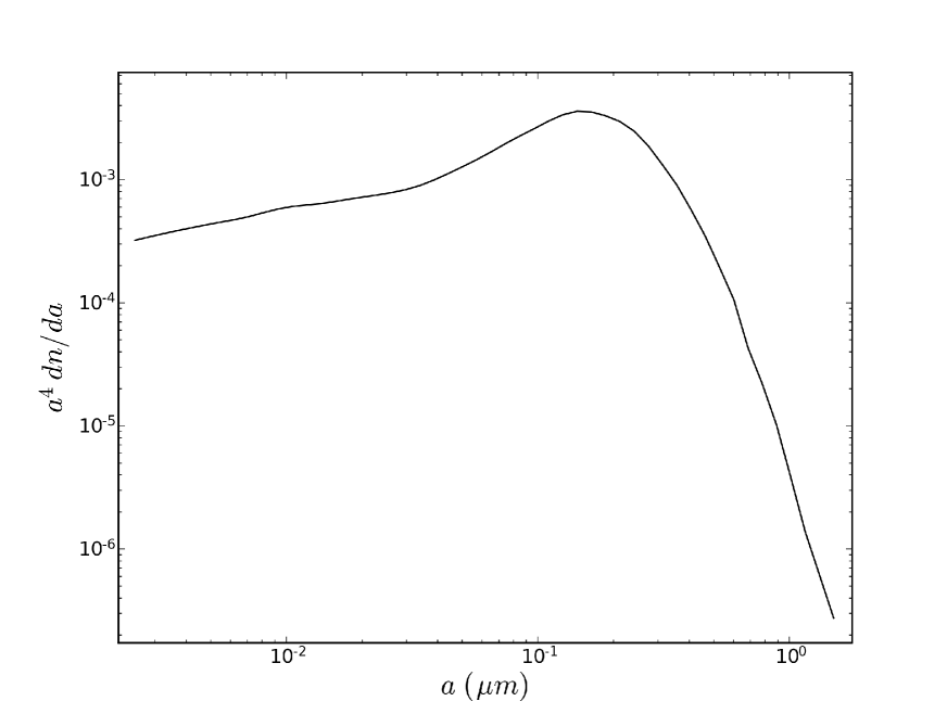
Figure 7.1: Size distribution of porous grains in the ISM, from Clayton et al. (2003). Compact grain distributions of Weingartner & Draine (2001) are shown in Figure 2.3.

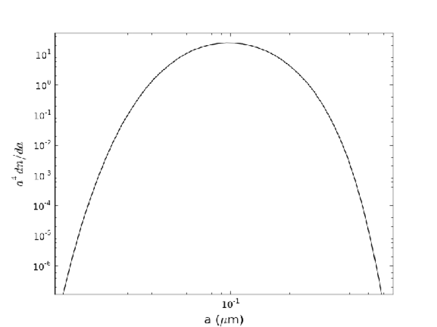
Figure 7.2: Size distribution of porous grains in the ISM, from Mathis (1996). Eq. (3) of his paper gives the functional form of the distribution as $dn/da\propto a^{-\alpha_{0}}exp[-(\alpha_{1}a+\alpha_{2}/a+\alpha_{3}a^{2})]$, where $\alpha_{0}$ = 3.5, $\alpha_{1}$ = 0.00333 $\mu$m^-1, $\alpha_{2}$ = 0.437 $\mu$m, and $\alpha_{3}$ = 50 $\mu$m^-2.

The size distribution of porous grains is unknown, because most interstellar extinction studies have been interpreted with compact grain models (Weingartner & Draine, 2001). There are only a few porous grain models available in the literature, and there are often significant discrepancies between them. For this work, I show results for two models. The primary model is a slightly modified version of that from Clayton et al. (2003), shown in Figure 7.1. This model consists of grains in a distribution from 0.0025 to 1.5 $\mu$m consisting of 50% vacuum, 33.5% astronomical silicate (MgFeSiO₄, whereas the original Clayton et al. (2003) model uses 28.5% pyroxene ([Fe_0.6Mg_0.4]SiO₃]) and 5% oxide ([Fe_0.4Mg_0.6]O)), and 16.5% amorphous carbon. I also show results in Chapter 8 from a second model, taken from Mathis (1996), which contains 15% of the mass in grains contained in a small population ($<$ 0.01 $\mu$m) of compact silicate grains. For the other 85%, I use a composite grain consisting of 50% vacuum and 50% solid material, where the solid material is made up of silicate and graphite in the approximate fractions in which they are found in the ISM of the Milky Way or LMC, as appropriate. The size distribution of porous grains in this model is shown in Figure 7.2. 50% vacuum is chosen for two reasons: 1) for ease of comparison to the Clayton model above; and 2) it likely represents the extreme (Heng & Draine, 2009) of interstellar grain porosities (although Voshchinnikov et al. (2006) reports that grains may be as high as 90% porous, using an MLS approach). The parameter space one can explore here is vast, and composite grains need not even be limited to the astronomical silicates and carbonaceous grains I have listed above. Whatever the distribution, compositeness, and porosity of interstellar grains is, I have written the code in such a way that any changes can be easily incorporated.

7.2.2 Collisional Heating and Sputtering of Porous Grains

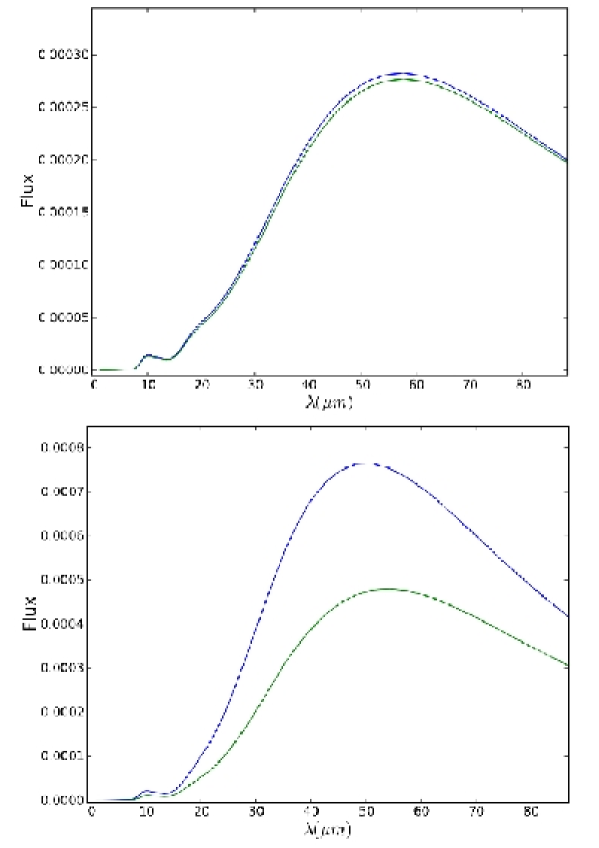
Figure 7.3: The impact of proton heating of grains for slow ($\sim 1000$) and fast ($\sim 3000$ km s^-1) shocks. For slow shocks, the difference between proton heating and no proton heating is hardly noticeable, but for fast shocks it becomes quite significant. Top: Thermal spectrum of warm grains heated behind slow non-radiative shock. Blue curve shows spectrum with $T_{p}$ = 1 keV, $T_{e}$ = 0.5 keV, Green curve shows $T_{p}$ = 0 keV, $T_{e}$ = 0.5 keV. Bottom: Same as top, but for fast non-radiative shock. Blue curve shows spectrum with $T_{p}$ = 20 keV, $T_{e}$ = 1 keV, Green curve shows $T_{p}$ = 0 keV, $T_{e}$ = 1 keV.

In addition to having different optical properties, porous grains are heated and sputtered differently than their solid counterparts. As a simple example, consider a given mass $M$ of dust grains in two populations: one population of solid (compact) silicate grains, all of radius $a=0.05\ \mu$m, and another of 50% porous silicate grains (with the other 50% vacuum), also all of radius $a=0.05\ \mu$m. Because half of the volume of porous grains is occupied by vacuum, the mass per grain is half that of the compact grains. In order to contain the same amount of total mass, $M$, there must be in total twice as many porous grains as compact. Now consider how these grains would be heated by a plasma. For this example, I choose a plasma of number density $n_{H}$ = 2.0, $T_{e}$ = 1 keV, and a total dust mass of $10^{-3}\ M_{\odot}$. I ignore heating by protons and consider only heating of grains by electrons (for all but the youngest SNRs, this is a reasonable approximation, see Figure 7.3). Sputtering is neglected.

Solid grains are heated to a higher temperature when subjected to the same plasma conditions. In a numerical model of the above example, 0.05 $\mu$m solid grains are heated to a temperature, $T_{dust}$, of $\sim 62.3$ K and have a total IR luminosity of $8.85\times 10^{35}\ L_{\odot}$, while porous grains are heated to $\sim 57.3$ K and have a total IR luminosity of $1.15\times 10^{36}\ L_{\odot}$, for a model luminosity ratio $L_{porous}/L_{compact}=1.3$.

As an alternative example, I modify the porous grain population above to now contain the same mass per grain as the solid grains. For a porosity of 50%, this means that their radius must be larger by a factor of $(1-{\cal P})^{-1/3}=1.26,$ so the porous grains now have radius $a=0.63\ \mu$m. In this example, the number, $N_{gr}$, of radiating grains is identical. Under the same plasma conditions from above, this porous grain population is heated to $T_{dust}=56.5$ K, and has a total luminosity of $1.09\times 10^{36}\ L_{\odot}$ in the model, for a luminosity ratio $L_{porous}/L_{compact}=1.23$.

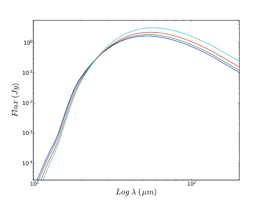
Figure 7.4: Comparison of model spectra from 10-200 $\mu$m for silicate grain size distributions of varying porosity. Blue: Compact silicate grains; Green: 10% porous silicate grains; Red: 25% porous; Cyan: 50% porous. Size distribution of Clayton et al. (2003) assumed, heating model (identical plasma conditions for all grain populations) described in text. Sputtering is neglected to highlight differences by heating only.

As a result of the equilibrium temperature being lower for porous grains, more heating is necessary to fit the same spectrum with a porous grain model than a solid grain model. For a fixed plasma temperature, this can only be achieved by increasing the post-shock density. When using dust as a density diagnostic, this has significant effects on inferences for the pre-shock density and compression ratio of the shock. Raising the post-shock density for a given X-ray emission measure must lower the pre-shock density (and thus, the gas mass swept-up by the forward shock). A porous grain model fit to the same spectrum will require a lower dust mass and gas mass. This is explored further with respect to model spectral data from SNRs in Chapter 8. In Figure 7.4, I show model spectra for compact, 10%, 25%, and 50% porous silicate grains heated under the conditions assumed above. These spectra are calculated over the entire grain size distribution of Clayton et al. (2003).

To include the effects of sputtering for porous grains, we assume that the sputtered yield from a porous grain is equal to that of a compact grain. For composite grains, a weighted harmonic mean of the sputtering rate for each grain component is used.

7.3 Energy Deposition Rates for Ions

If electrons and ions are at the same temperature, grains will be heated predominantly by electrons, since their velocities are much higher. In fact, in many SNRs heating by protons can be virtually neglected as a heating source for grains. However, it is often not the case in SNRs that there is a temperature equilibration between these particle species. In the simplest model of a collisionless shock, there is a significant temperature difference between protons and electrons, due to the fact that protons have a much higher mass. In reality, the situation is much more complicated than that, with contributions from collisionless heating at the shock and heating in the precursor. Nonetheless, observations show that, for fast shocks, protons are hotter than electrons. Recent evidence has shown that the post-shock ion/electron temperature ratio increases as $v_{s}^{2}$ (Ghavamian et al., 2007). In the case of fast shocks (i.e. shocks of a few thousand km s^-1 or more), heating by protons can have a significant effect, as shown in Figure 7.3.

If heating by protons is to be considered, then energy deposition rates must be properly accounted for in a heating model. Generally speaking, when dealing with gas at high temperatures, both protons and electrons deposit only a fraction of their energy into a grain, a fraction which depends on both the grain radius and the temperature of the impinging particle. This deposition function is represented by $h(a,T)$ in eq. 17. Aside from its dependence on $a$, the grain radius, and $T$, the temperature (or energy) of the particle, the amount of energy deposited by an impinging particle depends on the stopping power of the grain material. From the stopping power, one can calculate the projected range of an impinging particle into the grain. If this projected range is larger than the path traveled through the grain material, then the particle will exit the other side of the grain, having only deposited some of its energy. If the projected range is shorter than the path traveled, the particle will be stopped, and will deposit all of its energy into the grain. (Actually, for electrons, the total energy deposited only reaches about 0.875 of the initial energy, due to reflection from the surface of the grain (Dwek, 1987).) As an approximation to the total length traversed through the grain, I follow the standard in the field of approximating the average distance through a grain as being $R=\frac{4}{3}a$, which is the average path length through a sphere.

The stopping power (energy loss per unit path length) and projected range (average length traveled by a particle into a material) for both electrons and protons into a given grain are generally given by analytic expressions approximating experimental data. For electrons, these expressions fit the experimental data to within 15% for the energy range of 20 eV to 1 MeV (Dwek, 1987). For protons and alpha particles, the approximate projected range, based on experimental data from Andersen & Ziegler (1977) and Ziegler (1977), is given by Draine & Salpeter (1979) as

$$R_{H}=3\times 10^{-6}(E/keV)\ {\rm g\ cm}^{-2},R_{He}=0.6R_{H},$$ (29)

where $\rho$ is the mass density of the grain. The authors caution that this expression is valid only for $E<100$ keV. I raise here two questions: 1) Are these approximations appropriate for energies at or exceeding the 100 keV threshold (as may well be the case in very young SNRs with shock speeds exceeding 6000 km s^-1)? 2) These approximations are based on data over 30 years old; are they still valid?

7.4 Ion Heating of Grains in Fast Shocks

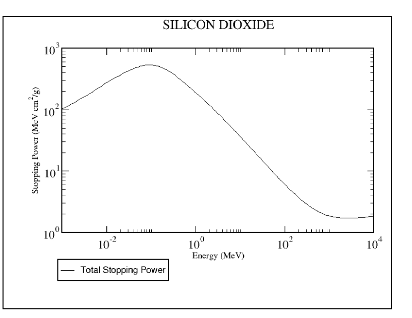
Figure 7.5: Stopping power divided by mass density, $\rho$, of a proton in silicon dioxide (SiO₂) as a function of proton energy. Taken from the NIST PSTAR database (see text).

To answer both of these questions, I turn to more recent laboratory data on the stopping power of protons and alpha particles in various materials, obtained from the online PSTAR and ASTAR databases published and maintained by the National Institute of Standards and Technology. These databases are freely available online. In Figure 7.5, I show the stopping power of a proton in silicon dioxide as a function of energy. The stopping power turns over at $\sim 100$ keV. Since, for an extremely fast shock, there will be a significant population of protons with energies in this range, this turnover should be properly accounted for in calculating the projected range of the particle.

Interstellar grains are more complicated than silicon dioxide (although it is possible that SiO₂ is a minor component of ISM dust). Since the NIST databases only have information available for actual materials that can be measured in the lab, materials like “astronomical silicate (MgFeSiO₄)” are not available. The individual stopping powers for the constituent elements are available, however, and can be combined to approximate the stopping power for a grain of arbitrary composition. To do this, I use “Bragg’s Rule” (Bragg, 1905), given by

$$S(A_{m}B_{n})=m\cdot S(A)+n\cdot S(B),$$ (30)

where $S(A_{m}B_{n})$ is the total stopping power of a molecule $A_{m}B_{n}$, and $S(A)$ and $S(B)$ are the stopping powers of the individual constituents. Since Mg is not included in the NIST database, I use the results of Fischer et al. (1996). Thus, for MgFeSiO₄, one has

$$S(MgFeSiO_{4})=S(Mg)+S(Fe)+S(Si)+4\cdot S(O).$$ (31)

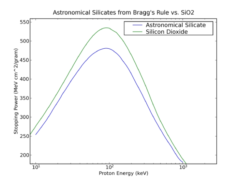
Figure 7.6: Stopping power of astronomical silicate, as calculated from Bragg’s Rule (see text). For comparison, the stopping power of SiO₂ obtained from the NIST PSTAR database is also shown.

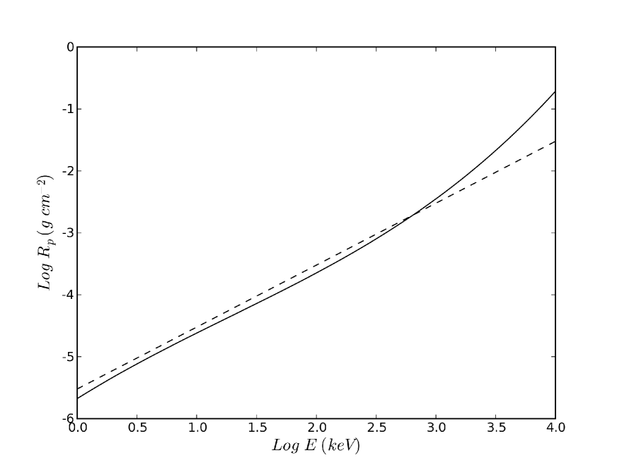
Figure 7.7: Projected range of a proton for MgFeSiO₄ as a function of energy. Solid curve is calculation described in text using Bragg’s rule; dashed curve is approximation of Draine & Salpeter (1979) that is valid at E $<$ 100 keV. The slight discrepancy at low energy is result of approximations in Bragg’s rule and in Draine & Salpeter (1979).

In Figure 7.6, I show the stopping power of MgFeSiO₄, derived via Bragg’s rule. The calculated projected range for protons based on this stopping power is shown in Figure 7.7, along with the approximation from eq. 27 above. The projected range curves I show are given by the following polynomial expressions in logarithmic space, where $E$ is the energy of the impinging particle in keV:

Protons

$$\log\ (R_{H,silicate})=0.053\ \log^{3}\ (E)-0.202\ \log^{2}\ (E)+1.21\ \log\ (E)-5.68$$ (32)

$$\log\ (R_{H,graphite})=0.053\ \log^{3}\ (E)-0.158\ \log^{2}\ (E)+0.961\ \log\ (E)-5.46$$ (33)

Alpha Particles

$$\log\ (R_{He,silicate}) = 3.78\times 10^{-3}\ \log^{5}\ (E)-8.79\times 10^{-3}\ \log^{4}\ (E)-4.25\times 10^{-2}\$$

$$\log^{3}\ (E)+6.25\times 10^{-2}\ \log^{2}\ (E)+1.04\ \log\ (E)-5.79$$

$$\log\ (R_{He,graphite}) = 3.33\times 10^{-3}\ \log^{5}\ (E)-6.13\times 10^{-3}\ \log^{4}\ (E)-3.46\times 10^{-2}\$$

$$\log^{3}\ (E)+3.03\times 10^{-2}\ \log^{2}\ (E)+0.966\ \log\ (E)-5.76.$$

Ultimately, the purpose of calculating the projected range of a particle into a grain is to determine how much energy is deposited into the grain by an impinging particle. If a particle exits the grain with energy $E^{\prime}$, then we can define $\Delta E$ = $E-E^{\prime}$, and the fractional energy deposited as $\Delta E/E$. This function is generally referred to as $\zeta(a,E)$, and the grain heating efficiency function, $h(a,T)$, is given by Dwek & Werner (1981) as

$$h(a,T)=\frac{1}{2}\int_{0}^{\infty}x^{2}\zeta(a,E)e^{-x}dx,$$ (34)

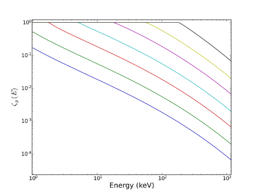
Figure 7.8: $\zeta_{p}(a,E)$, the fractional energy deposited by a proton into a silicate grain as a function of particle energy. From bottom-left (blue) to top-right (black), curves represent grains of radius 0.001, 0.003, 0.01, 0.03, 0.1, 0.3, and 1.0 $\mu$m.

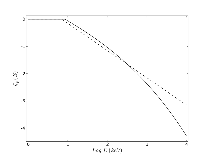
Figure 7.9: Zeta function for a single grain of 0.05 $\mu$m radius. Solid curve is calcuation described in text, dashed curve is approximation of Dwek & Werner (1981) (see text).

where $x=E/kT$. In Figure 7.8, I show calculations of $\zeta_{p}(a,E)$ for several grain sizes, and in Figure 7.9, I show $\zeta(E)$ for a single grain of radius 0.05 $\mu$m compared with the analytic approximation from Dwek & Werner (1981), given by

$$\zeta(a,E)=E^{*}/E\mbox{ for}\ E>E^{*},$$ (35)

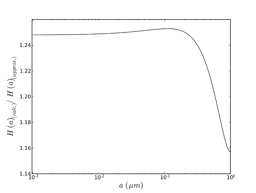
Figure 7.10: Ratio of proton heating rate of a silicate grain from calculations in this work to approximations from Draine & Salpeter (1979) & Dwek & Werner (1981) for an impinging particle energy of 100 keV, as a function of grain radius.

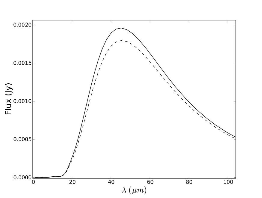
Figure 7.11: Comparison of spectra produced in dust heating model for protons of 100 keV. Solid line: spectrum assuming proton projected ranges calculated in Section 7.5. Dashed line: spectrum assuming analytical approximation to proton projected range from Draine & Salpeter (1979). Electron heating ($T_{e}$ = 2 keV) is included in this model.

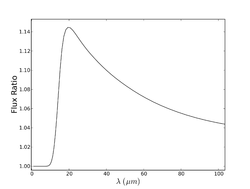
Figure 7.12: Ratio of spectra from Figure 7.11.

where $E^{*}$ is given by Draine & Salpeter (1979) as $E^{*}$(keV) = 133$a$ and 222$a$ ($a$ in $\mu$m) for protons and alpha particles, respectively. Of course, the ultimate question is how much these improved energy deposition rates matter. In Figure 7.10, I show the ratio of the heating rate, $H(a,T)$, calculated from the NIST energy deposition rates and that calculated from the analytical approximations of Draine & Salpeter (1979) and Dwek & Werner (1981), for a proton temperature of 100 keV, which is relevant for fast shocks such as those seen in SNR 0509-67.5 (see Chapter 8). Figure 7.11 shows a comparison of the spectra of grains heated behind such a shock, for both the modified energy deposition rates described above and the analytical approximations. Figure 7.12 shows the ratio of the spectra. The main difference is in the 18-40 $\mu$m range, but the maximum difference is only $\sim 15$%, which is roughly comparable to the errors in fitting models to data (see Section 2.9.1). The use of analytical approximations to proton heating rates should be valid for most cases. Nonetheless, I use the modified rates in reporting results in Chapter 8.

7.5 Non-thermal Sputtering of Grains Due To Gas-Grain Motions

On the other end of the SNR age spectrum are old remnants whose shock speeds are much lower, and the above issues with proton heating are irrelevant. In fast shocks, sputtering is mostly due to the thermal motions of the particles in the gas bombarding the grain. For slow shocks, however, an additional sputtering component is present that arises from the relative gas-grain motions in the post-shock region. Dust grains in the ISM typically have a low charge-to-mass ratio when compared with ions. This means that they are largely unaffected by the passage of the shock front over them. In their frame of reference, though, they are suddenly thrust into a plasma with a bulk-velocity of $\frac{3}{4}v_{s}$, where $v_{s}$ is the shock speed. They are eventually brought to a rest in the frame of the gas due to the drag force from collisions with ions, but this takes a non-negligible amount of time, during which their sputtering rate is increased. This sputtering is referred to as “non-thermal” sputtering, to contrast it with the case in which the sputtering is purely “thermal.” (This should not be confused with other uses of the phrase “non-thermal” in this thesis, which typically refer to the emission produced by a relativistic population of electrons.)

A particular case where this is relevant is in the Cygnus Loop, a 10,000-20,000 year old supernova remnant at a distance of $\sim 500-600$ pc. Shock speeds in the Cygnus Loop are 300-500 km s^-1, and the remnant as a whole is roughly 3 degrees in diameter. The entire shell was detected in soft X-ray bands by the ROSAT All-Sky Survey. Spitzer observations of a non-radiative shock on the northeast limb of the Cygnus Loop were obtained in 2005 December as part of Cycle 2 Guest Observer program 20743 (R. Sankrit, P.I.). ^† The target field was centered on $\alpha_{\rm{J2000}}$ = 20$\fh$ 54$\fm$ 35$\fs$, $\delta_{\rm{J2000}}$ = +32° 17′ 30″. The $24\,\mu$m observations included 12 frames and totalled 375 s. The field-of-view of the shocked region is about 5.7′ $\times$ 5.7′. The $70\,\mu$m images consisted of a $3\times 3$ raster obtained in the narrow field-of-view mode. For each position, 40 frames were obtained with a total exposure time of about 340 s. The overall field-of-view of the $70\,\mu$m image is about 8′ $\times$ 13′, and completely overlaps the $24\,\mu$m image field-of-view.

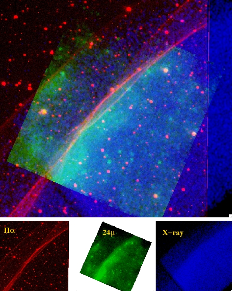
Figure 7.13: 3-color image of the P7 region of the Cygnus Loop. Red: H$\alpha$; Green: Spitzer 24 $\mu$m; Blue: Chandra X-ray.

A three-color image of the non-radiative shock is shown in Figure 7.13. Red is an H$\alpha$ image obtained at the Mt. Hopkins Whipple Observatory 1.2m telescope, green is the $\>{\it Spitzer}$ $24\,\mu$m image, and blue is an exposure-corrected 0.35–2.0 keV Chandra image made from the ACIS-S3 data (ObsID 2821) using CIAO 3.4. The H$\alpha$ emission traces a narrow zone ($\sim 10^{14}$ cm thickness) just behind the shock front. The infrared emission arises in a more extended zone behind the shock front. The X-ray emission comes from the entire post-shock region where the gas initially is heated to a temperature of a few times $10^{6}$ K. As the gas ionizes, the X-ray emission is dominated by different species: Si and Fe make the major contribution just behind the shock, and O and Ne further downstream. A fainter shock is clearly seen ahead of the main shock, near the left edge of the $24\,\mu$m image field of view. The three images are shown separately along the bottom of the figure.

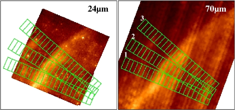
Figure 7.14: Spitzer 24 and 70 $\mu$m images of the Cygnus Loop, with analysis regions overlaid.

The $\>{\it Spitzer}$ $24\,\mu$m and $70\,\mu$m images are shown in Figure 7.14. Fluxes were measured along each of the three strips shown on these images. The strips were chosen to be perpendicular to the shock front as seen in the $24\,\mu$m image. Each strip is about 60″ across and each box is 20.33″ wide. This corresponds to 22 pixels and 8 pixels, respectively in the $24\,\mu$m image and about 14 pixels and 5 pixels in the $70\,\mu$m image.

The total fluxes within each box were calculated for the MIPS images by summing the data values (in MJy/sr) for pixels contained in the box multiplied by the solid angle subtended. These were used to construct flux profiles along each strip. The background in the $24\,\mu$m image is about 3 mJy/pixel, and fairly uniform over most of the detector. We subtract this value off each pixel to obtain background subtracted profiles. The uncertainty in the background value is $\sim 0.003$ mJy/pixel, or $\sim 0.53$ mJy in each box. This uncertainty translates to about 5% error in the flux measurement near the peak of the $24\,\mu$m emission. The exception to the near-uniform background is in the region around the Northern corner of the FOV, where the background is lower and more variable. There is no such difference associated with that part of the sky in the $70\,\mu$m image. This suggests that the anomaly is due to the $24\,\mu$m detector and does not have any astrophysical significance. Therefore, we avoid the region in our analysis.

The background in the $70\,\mu$m image varies across the field of view. For each profile, we fit a low-order polynomial to the boxes near the ends and used that for the background. We varied the background fit in several reasonable ways - using different numbers of points, different order polynomials (including constant value backgrounds) - to see how these changes affected the measured fluxes. We find that uncertainties in the background contribute an error of about 5% to the flux measurements near the peaks of the profiles.

To model non-thermal sputtering, we use formulae for the gas drag force found in Draine & Salpeter (1979), where we neglect the Coulomb drag, as this should be negligible in a hot, X-ray emitting plasma. As a grain slows down, sputtering causes its mass and radius to decrease. The sputtering rate is given by Nozawa et al. (2006). The coupled equations for the grain radius and velocity are solved with standard numerical ordinary differential equation solvers. Since grain gyroradii are much smaller than the spatial scales of interest, we assume that dust and gas motions are tightly coupled, i.e. grains gyrate with small (and negligible) gyroradii around magnetic fields frozen into and moving with the shocked gas. As in previous work on Galactic and LMC remnants, we use a plane-parallel approximation for the shock structure. The most important shock parameters are the pre-shock density and the shock speed, $v_{s}$, which determine the post-shock temperature and density through the standard strong-shock jump conditions. The electron and ion temperatures in the post-shock region are expected to be equal for the relatively slow shock being studied (Ghavamian et al., 2001). In contrast with previous work, the shock structure here is resolved, and each of the spatial bins can be conveniently described by $\tau_{l}$ and $\tau_{u}$ ($\tau\equiv\int_{0}^{\tau}n_{p}dt$), the lower and upper “sputtering” ages bracketing its position.

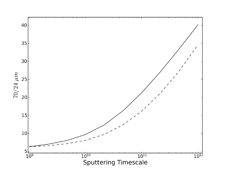
Figure 7.15: 70/24 $\mu$m flux ratio as a function of sputtering timescale for a temperature of $T_{p}$ = $T_{e}$ = 0.3 keV, appropriate for the Cygnus Loop. Solid black curve includes effects from both thermal and non-thermal sputtering, dashed black line includes only thermal sputtering.

At the relatively low plasma temperatures that we obtain in the Cygnus Loop shocks, non-thermal sputtering is expected to contribute significantly to the dust destruction (e.g. Dwek, Foster, & Vancura, 1996). In order to check this, we ran a grid of models that included only thermal sputtering. The $70\mu$m to $24\mu$m flux ratios predicted in these models were about 40% lower than in the original set, and failed to reproduce the observed ratios. Our data clearly show that non-thermal sputtering is an important process for dust destruction in shocks with speeds $\lesssim$500 km s^-1.^‡ In Figure 7.15, I show a plot of the 70/24 $\mu$m ratio behind the shock for identical conditions, with non-thermal sputtering turned on and off.

7.6 Sputtering Rates for Small Grains

The sputtering rate for small grains is much more uncertain that that for large grains. For large grains, the “semi-infinite solid” approximation can be used, which is what most laboratory experiments can measure. This approximation (which is typically fine for industrial applications) assumes that all sputtering comes from the surface of the grain where the impact takes place. With dust, however, this is not always a valid approximation. If the grain is small enough, sputtering can occur from not only the front side of the grain, but the back and sides as well. To account for this, we use the “enhanced” sputtering rates of Jurac et al. (1998). Even this enhancement may not paint the full picture though, as for really small grains (where a grain is considered “small” if $R_{p}>\frac{4}{3}a\rho$), the sputtering yield may again be decreased due to the incomplete deposition of energy from protons into the grain (Serra Dìaz-Cano & Jones, 2008). To account for this, we make the assumption that, to first order, the sputtering rate is directly proportional to the energy deposited into the grain, which drops with decreasing grain size. An example of the sputtering rate as a function of grain size, taking all three of these effects into account, is shown in Figure 7.16.

7.7 Liberation of Elements into Gaseous Phase

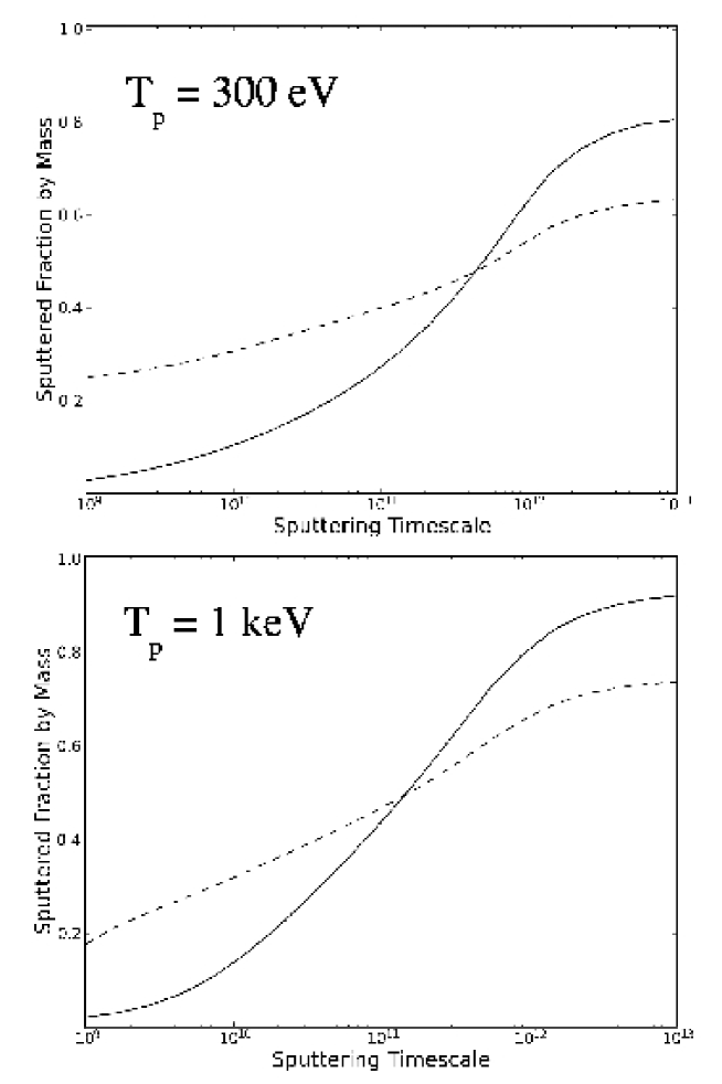
Figure 7.17: Sputtered fraction, by mass, for grains as a function of sputtering timescale, $\tau_{p}=\int_{0}^{t}n_{p}dt$. Solid black line: Silicate grains; Dashed line: Graphite grains. Plots are for dust in the ISM of the Milky Way.

As dust is eroded via sputtering, the atoms ejected from the grain do not simply disappear. They are “liberated” back into the gaseous phase and are equilibrated with their surroundings in the hot post-shock region. The refractory elements that make up dust grains (C, O, Mg, Si, Fe, etc.) are the same elements whose lines are commonly seen in X-ray spectra of SNRs. If sufficient amounts of these atoms are injected into the post-shock gas from grain sputtering, it is possible to see the effect on X-ray spectra as a function of distance behind the shock. In Figures 7.17 and 7.18, I show the amount of material sputtered for silicate and graphite grains as a function of the sputtering timescale (which, in a plane-shock model, is proportional to the distance behind the shock or the time since shocked) for a range of post-shock proton temperatures. The sputtered fraction listed in the figures is dependent on the grain size distribution assumed. It is given by mass, and can thus be converted to absolute masses of various elements, if the total dust mass needed to fit the observed fluxes or spectra can be determined.

7.8 Summary

Since SNRs were first detected in the mid-IR with IRAS more than 25 years ago, numerous authors have worked to model the emission seen with models of collisionally heated dust. Despite this work, there is still much that is unknown about interstellar dust, and a lot of physics that is known that is still not properly incorporated into such models. I have built on previous work in this field by extending models (Borkowski et al., 1994) to include the effects listed above.

Specifically, I have developed a code to approximate the optical constants for a grain composed of arbitrary amounts of astronomical silicate, graphite, amorphous carbon, and vacuum. This code could be extended in the future, if necessary, to incorporate other grain materials. The code also calculates modified heating and sputtering rates for these composite/porous grains. I have also incorporated more up-to-date energy deposition rates for ions, particularly important in the case of very fast shocks, such as those seen in Cas A or SNR 0509-67.5. For slow shocks, such as those in the Cygnus Loop, I have extended the code to include effects of non-thermal sputtering caused by relative motions between gas and dust grains. The sputtering rate for small grains has been updated to reflect the amount of energy deposited into a grain. Liberation of elements from grains can be followed in the code as a function of sputtering timescale. If some parameters of the SNR are known, such as the distance to the object, this sputtering could be followed in terms of a post-shock distance and/or absolute mass scale. This injection of elements into the gaseous phase could be compared directly with X-ray fits for post-shock regions in sufficiently well-resolved SNRs.

Current and future generations of IR telescopes, such as the Stratospheric Observatory for Infrared Astronomy (SOFIA), the Wide-field Infrared Survey Explorer (WISE), the Herschel Space Observatory, and the James Webb Space Telescope, as well as X-ray telescopes like the International X-ray Observatory, will allow testing of these models, as will archival study of Spitzer, Chandra, and XMM-Newton data.

Figure 7.16: Sputtering rate as a function of grain radius, where sputtering is done by protons with energy 10 keV. Rates used in code shown in blue, bulk sputtering approximation shown in green. Increase in rate from $10^{-2}-10^{-1}$ $\mu$m due to enhancement of sputtering for small grains, dropoff short of $\sim 10^{-2}$ due to decreased energy deposition rate for energetic particles. Same as Figure 2.8.

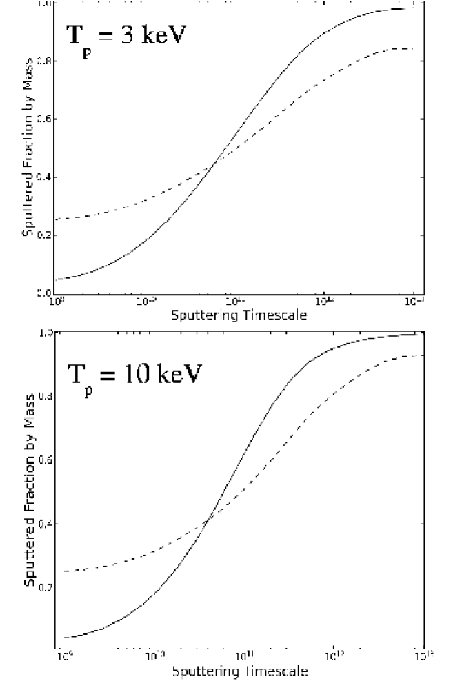
Figure 7.18: Same as Figure 7.17, but for post-shock proton temperatures of 3 and 10 keV.

8 Spitzer IRS Observations of Two Young Type Ia Supernova Remnants in the LMC

This chapter is part of a manuscript in preparation for submission to the Astrophysical Journal.

8.1 Introduction

Supernova remnants (SNRs) provide a laboratory to study various aspects of interstellar medium (ISM) evolution across the whole electromagnetic spectrum. With the advent of high spatial resolution telescopes in both the X-ray and infrared (IR) regimes, it is possible to probe the interaction of the rapidly moving shock wave with the dust and gas of the surrounding ambient medium, in addition to studying the ejecta products of the SN itself. The expanding shockwave sweeps up and heats gas to $10^{6}-10^{7}$ K, causing it to shine brightly in X-rays. Dust grains embedded in the hot, shocked plasma are collisionally heated, causing them to radiate at IR wavelengths. The same collisions with hot ions slowly destroy grains in the process via sputtering. Because the physical processes behind X-ray and IR emission are related, a combined approach to studying SNRs using both energy ranges can reveal more information than either could on its own.

To better characterize IR emission from SNRs, we conducted an imaging survey with the Spitzer Space Telescope of $\sim 40$ known SNRs in the Large and Small Magellanic Clouds. The Clouds were chosen because of their known distance and relatively low Galactic IR background. We conducted spectroscopic follow-up with the Infrared Spectrograph (IRS) on Spitzer on several remnants during cycle 4 of observations. We report here on IRS observations of two of these objects, SNRs B0509-67.5 (0509) and B0519-69.0 (0519). Both are remnants of thermonuclear SNe (Smith et al., 1991) that have fast, non-radiative shocks (several thousand km s^-1) (Tuohy et al., 1982; Ghavamian et al., 2007). There is no evidence in either for slower, radiative shocks. They are both located in the LMC, at the known distance of $\sim 50$ kpc. In addition, both have ages determined from light echoes (Rest et al., 2005) to within 33%, 0509 being 400 $\pm 120$ and 0519 being 600 $\pm 200$ years old. They are nearly identical in size, having an angular diameter of $\sim 30$”, which corresponds to a physical diameter of $\sim 7.3$ pc.

In Borkowski, et al. (2006) hereafter Paper I, we used photometric detections of both SNRs to put limits on the post-shock density and the amount of dust destruction that has taken place behind the shock front, as well as put a limit on the dust-to-gas mass ratio in the ambient medium, which we found to be a factor of several times lower than the standard value for the LMC of $\sim 0.25$% (Weingartner & Draine 2001, hereinafter WD01). These limits, however, were based on only one IR data point, the 24 $\mu$m detection. With full spectroscopic data, we can place much more stringent constraints on the dust destruction and dust-to-gas mass ratio in the ISM. We also explore alternative dust models, such as porous and composite grains. Additionally, we examine archival data from the Reflection Grating Spectrometer (RGS) onboard the XMM-Newton X-ray observatory. The high spectral resolution of RGS allows us to separate lines from the ambient medium from those arising from reverse-shocked ejecta, giving us an emission measure (EM), or an upper limit, of the shocked ISM. The EM allows us to infer a pre-shock density, given information derived from IR fits.

8.2 Observations and Data Reduction

Both objects were fully mapped by the long wavelength (14-38 $\mu$m), low-resolution ($\Delta\lambda/\lambda$ $\sim 100$) (LL) spectrometer on Spitzer’s IRS. For 0509, we stepped across the remnant in seven LL slit pointings, stepping perpendicularly 5.1^′′ each time (5.1^′′ is half the slit width). We then shifted the slit positions by 56^′′ in the parallel direction and stepped across the remnant again, ensuring redundancy for the entire object. This process was repeated for each of the two orders of the spectrograph. Each pointing consisted of two 120-second cycles, for a total observing time of 6720 s.

For 0519, the process was identical in terms of number of positions and step sizes in between mappings, but each pointing consisted of four 30-second cycles, for a total observing time of 3360 s. The difference was due to the fact that 0519 is several times brighter in the wavelength range of interest, and we did not want to saturate the detectors.

The spectra were processed at the Spitzer Science Center using version 17.1 of the IRS pipeline. We ran a clipping algorithm on the data which removes both hot and cold pixels that are more than 3$\sigma$ away from the average of the surrounding pixels. To extract the spectra, we used SPICE, the Spitzer Custom Extraction tool. Once all datasets were extracted, we stacked spectra from the same spatial location, improving the signal-to-noise ratio of the sources. For background subtraction, we use the off-source slit positions that come when one of the two slit orders in on the source. In the end, we have seven (overlapping) background-subtracted spectra for each remnant. As we show in Section 8.3, this allows us to do spatially resolved spectroscopy, despite the fact that the remnants are only $\sim 30^{\prime\prime}$ in diameter.

We processed archival XMM-Newton RGS data from the XMM Science Archive with version 8.0 of the Science Analysis System (SAS) software for XMM. 0509 was observed on 4 July 2000 (Obs. ID 0111130201, PI M. Watson) for 36 ksec. 0519 was observed on 17 September 2001 (Obs. ID 0113000501, PI A. Brinkman) for 25 ksec. Since RGS is a slitless spectrometer, spatial information is degraded for extended sources, and the spectrum is smeared by the image of the source. In order to model RGS spectra, the response files generated by SAS must be convolved with a high-resolution X-ray image. For our purposes, we used archival broadband Chandra images, along with the FTOOL rgsrmfsmooth, to produce new response matrices.

8.3 Results

8.3.1 0509

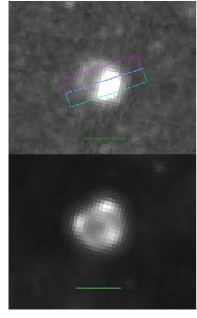
Figure 8.1: Top: MIPS 24 $\mu$m image of SNR 0509-67.5, overlaid with regions of spectral extraction as described in text, where magenta region is “faint” region and cyan marks “bright” region. Bottom: MIPS 24 $\mu$m image of SNR 0519-69.0. Green bar on both images corresponds to 30^′′. FWHM of MIPS 24 $\mu$m PSF is approximately 7^′′.

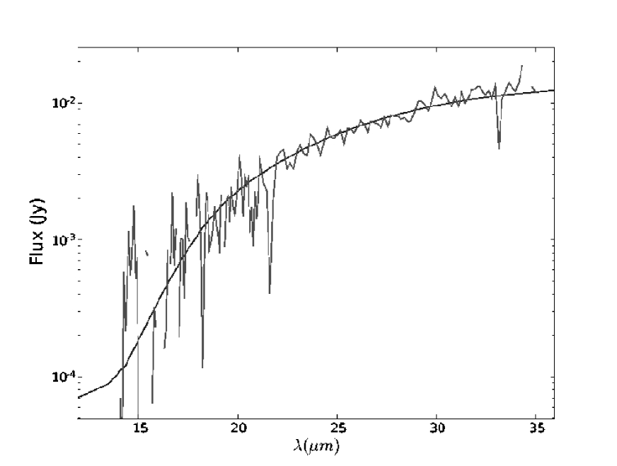
Figure 8.2: 14-35 $\mu$m IRS spectrum of the “faint” region of 0509, overlaid with model fit.

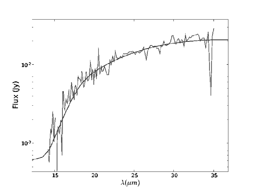
Figure 8.3: 14-35 $\mu$m IRS spectrum of the “bright” region of 0509, overlaid with model fit.

In Figure 8.1, we show the MIPS 24 $\mu$m images of 0509 and 0519, with overlays as described in the caption. Immediately obvious is the large asymmetry in 0509, where the remnant brightens by a factor of 5 between the faint NE hemisphere and the brighter SW. This is a much higher flux contrast than seen in Chandra broadband images, which show a modest factor of 1.5 between the two hemispheres. Using IRS, we are able to separate the remnant into 7 overlapping regions from which spectra were extracted. For our analysis, we chose two regions (shown on Figure 8.1) that do not overlap spatially and provide adequate signal to noise spectra. These regions roughly correspond to the bright and faint halves of the remnant, and the spectra are shown in Figure 8.2 and Figure 8.3. The ratio of integrated fluxes from 14-35 $\mu$m for the two regions is $\sim 2.5$. This differs from the factor of 5 measured from the photometric images because the slits are not exactly aligned with the bright and faint halves of the remnant, and because of the differences in the MIPS and IRS bandpasses.

A few obvious features immediately stand out about both spectra. First, there is no line emission at all seen in either spectrum. This is not unexpected, since the shocks in 0509 are some of the fastest SNR shocks known, at $\sim 6000$ km s^-1 (Ghavamian et al., 2007), and one does not expect any radiative cooling in the gas at such shock velocities. Second, though both spectra show continuum from warm dust, there are obvious differences in the spectra. An inflection around 18 $\mu$m can be seen in the spectrum from the bright half, while this feature is not as clear in the faint spectrum. We attribute this feature to the Si-O-Si bending mode in amorphous silicate dust. In Section 8.6, we will explore reasons for the different spectral shapes and the differences in brightness between the two halves of the remnant.

8.3.2 0519

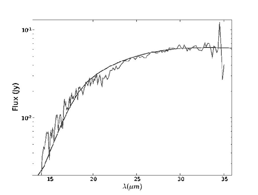
Figure 8.4: 14-35 $\mu$m IRS spectrum of SNR 0519-69.0, extracted from a slit placed across the middle of the remnant, free of emission from the bright knots seen in the 24 $\mu$m image; with model overlaid.

0519 does not show the large scale asymmetries that 0509 does, although three bright knots can be seen in the 24 $\mu$m image. These same three knots can be identified in both H$\alpha$ and X-ray images, where Chandra broadband data show that the three knots are prominent in the 0.3-0.7 keV band. From the MIPS 24 $\mu$m image, we measured the total flux from the three knots added together and found that collectively they represent only about 20% of the flux. Nevertheless, spectra extracted from slits that contain a bright knot do show differences in continuum slope from those extracted where no knots are present. We discuss our interpretation of these knots in Section 8.6. As with 0509, there are no lines seen in the IRS data (see Figure 8.4), as shock speeds are also quite high in this object.

8.4 IRS Fits

We now turn our attention to modeling the emission seen in IRS with numerical models of collisionally heated dust grains. We follow a procedure identical to that followed in our previous work on these objects; see previous chapters. A more complete description of models can be found there; see also Williams et al. (2006); Blair et al. (2007). Briefly, we model warm dust heated by collisions with electrons and ions, taking into account sputtering by ions, which destroys small grains and sputters material off large grains. We use a plane-shock model which superimposes regions of increasing shock age (or sputtering timescale) $\tau_{p}=\int_{0}^{t}n_{p}dt$, where $n_{p}$ is post-shock proton density, while keeping temperature behind the shock constant. Inputs to the model are an assumed pre-shock grain-size distribution, grain type and abundance, proton and electron density, ion and electron temperature. The code calculates the heating and sputtering for grains from 1 nm to 1 $\mu$m, producing a unique grain temperature and spectrum for each grain size. The spectra are then added in proper proportions according to the post-sputtering size distribution to produce a model spectrum that can be compared with observations. We use sputtering rates from Nozawa et al. (2006) with enhancements for small grains from Jurac et al. (1998). We assume that sputtering yields are proportional to the amount of energy deposited by incoming particles, accounting for partial transparency of grains to protons and alpha particles at high energies (Serra Dìaz-Cano & Jones, 2008), particularly relevant for 0509 and 0519. We assume that grains are compact spheres, but we also report results and implications if grains are porous (i.e. contain a filling fraction of vacuum $>$ 0).

In general, our method is to fix as many of the input parameters as possible, based on what is known from other observations. For instance, Rest et al. (2005) used optical light echoes to constrain the ages of both remnants, yielding ages of $\sim 400$ yrs. for 0509 and $\sim 600$ yrs. for 0519. Shock velocities are known approximately for both objects ($\sim 6000-7000$ km s^-1 for 0509 and $\sim 3800$ km s^-1 for 0519) (Tuohy et al., 1982; Ghavamian et al., 2007) from measurements of proton temperatures. The main “fitted” parameter that remains is the post-shock density of the gas, $n_{H}$, which can then be tuned to reproduce the shape of the observed IR spectra. The overall normalization of the model to the data (combined with the known distance to the LMC) provides the mass in dust. Since our models calculate the amount of sputtering that takes place in the shock, we can then determine the amount of dust present in the pre-shock undisturbed ISM. While we are sensitive only to “warm” dust, and could in principle be underestimating the mass in dust if a large percentage of it is too cold to radiate at IRS wavelengths, it is difficult to imagine a scenario where any significant amount of dust goes unheated by such hot gas behind the high-velocity shocks present in both remnants, particularly given the upper limits at 70 $\mu$m reported in Borkowski, et al. (2006) (and the fact that there are no radiative shocks observed anywhere in these remnants).

Although we have full spectral mapping of both objects, the width of the IRS slit at 10.5^′′ severely limits the amount of spatially resolved spectroscopy we can do on a remnant that is only 30^′′ in diameter, as both 0509 and 0519 are. Nevertheless, we do have several unique slit positions, and can use these to obtain spectra from various regions to explain the various asymmetries observed in both remnants. Because dust radiates as a modified blackbody spectrum, emission from a small amount of warmer dust can overwhelm that from a larger amount of colder dust, particularly at the wavelengths of interest here. We show in Figure 8.2 and Figure 8.3 extracted spectra from two regions of 0509, which we label the “bright” and “faint” portions of the remnant. If each of these two regions represents half of the object, this requires a density contrast of $\sim 4$ in the post-shock gas, with the higher density required in the “bright” region (higher densities means hotter dust, hence more short wavelength emission). Although it may be possible that a density gradient from the NE to the SW of this order does actually exist in the ambient medium surrounding 0509 (the angular size of 30^′′ in the LMC corresponds to a linear diameter of about 7 pc), the implications from this model lead to several scenarios which are unlikely and require an appeal to special circumstances.

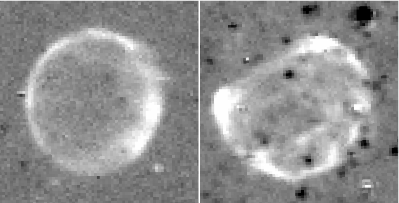
Figure 8.6: Star-subtracted H$\alpha$ images of 0509 (left) and 0519 (right). Note brightness enhancement in SW for 0509, and location of bright knots in 0519.

In comparing the MIPS image with images of the remnant at other wavelengths, one can clearly see an enhancement in the Chandra broadband image (Warren & Hughes, 2004) on the west side of the remnant. This enhancement is mostly present in the energy range containing Fe L-shell emission lines. The H$\alpha$ image, shown in Figure 8.6, shows a uniform periphery around the remnant, with the exception of a brightness enhancement in the SW, relatively well constrained to a small region a few arcseconds in size. If the H$\alpha$ image is smoothed to the resolution of the MIPS 24 $\mu$m image ($\sim 7^{\prime\prime}$), the result is morphologically similar to the 24 $\mu$m image. From these comparisons, we conclude that there is not an overall NE-SW density gradient in the ISM, rather, the ISM is mostly uniform except for the SW, where the remnant is running into a localized region of higher density. To obtain the conditions for the whole of the remnant, we fit a model to the “faint” region, freezing all parameters to those reported in Table 8.1 and allowing post-shock density to vary (which also causes the sputtering timescale to vary). If we assume a standard LMC dust model, we get a post-shock density of $n_{H}$ = 0.88 cm^-3.

Our assumption that the bright region of 0509 is the result of a more localized enhancement in density implies that the spectrum extracted from that region is then a composite of emission from the uniform parts of the remnant and from the small, denser region. Spitzer does not have the resolution required to isolate this dense region, but we can make a crude isolation by assuming that the two slit positions cover an equal surface area on the remnant, and subtracting the faint spectrum from the bright. The residual spectrum is of less than ideal signal-to-noise. Nevertheless, a fit to this spectrum implies a gas density of $\sim 7$ cm^-3, or about an order of magnitude higher than the rest of the remnant. A small region of hot dust outshines a more massive region of cooler dust at 24 $\mu$m, which explains the factor of 5 ratio in the flux between the two sides. X-rays from this object are dominated by ejecta, not swept-up ISM, and there are several factors to consider beyond density when considering the flux of H$\alpha$ coming from a region. Higher resolution observations at all wavelengths will shine more light on this issue.

For 0519 we have a similar scenario, except that instead of one bright region, we have three bright knots. As noted previously, these knots correspond spatially with knots seen in both X-rays and H$\alpha$ (see Figure 8.6). We adopt an identical strategy here, isolating spectra from slit positions that do not overlap with one of the bright knots. As it turns out, there is only one slit position in this object that is nearly completely free of emission from a knot, a slit position that goes directly across the middle of the remnant. The spectrum from this region is shown in Figure 8.4. We assume that the conditions within this slit position are indicative of the remnant as a whole. Using parameters found in Table 8.1, we obtain a post-shock density of $n_{H}$ = 8 cm^-3. We do not have adequate signal-to-noise to isolate one of the bright knots alone. However, we approximate the density required by noting that a fit to the entire slit position that contains the brightest of the three knots (the northernmost knot) requires a density that is higher by a factor of $\sim 2$. Given that this spectrum contains emission from both the uniform parts of the remnant and the bright knots, it is likely that the density in the knots themselves are perhaps a factor of $\sim 3$ higher that the more uniform parts of the remnant.

8.5 X-ray Modeling of RGS Data

Although dust models in the IR are a powerful diagnostic of the post-shock gas, they are insensitive to pre-shock gas conditions, while the total swept mass depends on this. X-ray modeling of SNR spectra, on the other hand, can provide a handle on the pre-shock gas through the emission measure (EM) of the gas, defined as EM = $\int_{0}^{V}fn_{e}n_{H}dV$, where $n_{e}$ and $n_{H}$ are the post-shock electron and hydrogen densities, respectively, $V$ is the emitting volume of hot gas, and $f$ is the filling fraction of the material. If the densities do not vary greatly over the emitting volume, the EM can be rewritten as EM = $n_{e}n_{H}V$. Determining the density directly from the EM can be done, but with the caveat that any clumping of the gas will bias the result, owing to the factor of $n^{2}$ in the definition.

If $n_{e}$ can be independently determined (such as through IR observations of warm dust), then it can be divided out of the emission measure, leaving only the product of n_H and $V$, which, regardless of any clumping effects, is simply the mass in gas swept up by the forward shock. The volume of these remnants is well-known, thanks to their resolved angular size and location in the LMC ($D$ = 50 kpc). Thus, it is a straightforward calculation to determine the average pre-shock density that the forward shock has encountered over its lifetime. A caveat to this approach is that the swept-up gas must still be hot enough to emit X-rays, but for remnants at a relatively early stage of evolution, as is the case for both 0509 and 0519, this is not a concern.

The difficulty in this approach lies in disentangling X-ray emission from the shocked ambient medium from that arising from reverse-shocked ejecta. For large remnants, this could be done spatially using CCD spectra, but both 0509 and 0519 are $\sim 30^{\prime\prime}$ in diameter with the ejecta not well separated from the shocked ISM, rendering such an approach impossible. For 0509, previous studies (Warren & Hughes, 2004; Badenes et al., 2008) have used Chandra CCD spectra to model emission from the remnant, but these studies are subject to the inherent difficulty in using CCD spectra to disentangle ISM and ejecta emission. An alternative approach is to take high-resolution spectra from grating spectrometers, such as RGS on XMM-Newton. If lines can be identified as arising only from shocked ambient medium, then model fits to these lines would provide an EM for the ISM. This can be most easily done with N lines, as virtually no N is produced in type Ia explosions. Kosenko et al. (2008) used this approach to fit the 24.8 Å N Ly-$\alpha$ line in the spectrum of 0509, but we find that this line is very weak and unconstraining to the fitting procedure used here. Here we fit O and Ne lines seen in RGS spectra and attribute them to the shocked ambient medium, since neither element appears to be produced in great abundance in type Ia SNe (Marion et al., 2009).

8.5.1 0509

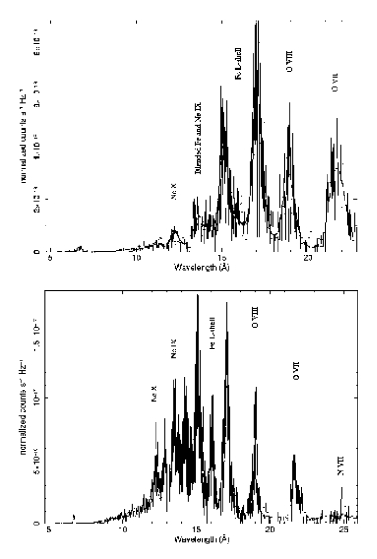
Figure 8.5: Top: XMM-Newton RGS spectrum of 0509-67.5, from 5-23 Å. Bottom: RGS spectrum of 0519-69.0, from 5-27 Å; models overlaid in both as described in text.

The preferred explosion model for 0509, DDTa (Badenes et al., 2008), synthesizes 0.04 $M_{\odot}$ of O, the least of any of the explosion models considered for that remnant. In Figure 8.5, we show RGS spectra from both remnants. Fe L-shell lines dominate the spectra, but strong lines from both H- and He-like O are clearly visible in both cases at 18.97 and 21.7 Å. Ne lines blend together with Fe lines between 12 and 14 Å; we attempt to disentangle them as described below. Our procedure for modeling lines is similar to that in Blair et al. (2007) for Kepler’s SNR; see Appendix A for a more detailed description. An additional step we took here was to first fit a model to only the data between 14-18 Å, which are dominated by iron lines. We then added a component (vpshock model with fixed normal LMC abundances with ionization timescale and normalization free) to fit the data around Ne and O lines, fitting the data from 9-23 Å with the two models. These two models can be thought of as the “ejecta” model and the “ISM” model. We use two absorption components, one resulting from galactic absorption column density, $N_{H}$, equal to 5 $\times$ 10²⁰ cm^-2, and one from the LMC (at fixed LMC abundances), equal to 2 $\times$ 10²⁰ cm^-2 (Warren & Hughes, 2004). The “ejecta” model is important only for disentangling Ne and Fe emission, it has no significant effect on fitting O lines. In the “ISM” model, we freeze the electron temperature to 2 keV, roughly the number one gets from Coulomb heating models behind the shock (the dependence of the emission measure of the gas on the electron temperature is small). We introduce an additional line smoothing parameter to both models to allow for the fact that lines are broadened by Doppler motions. For 0509, we find that relative fluxes in O VII, O VIII, Ne IX, and Ne X are well fit (reduced $\chi^{2}$ = 1.2 for 235 d.o.f.) by a model with $\tau_{i}=\int_{0}^{t}n_{e}dt$ = 3.5 (3.1, 4.0) $\times$ 10¹⁰ cm^-3 s and EM = 2.0 (1.9, 2.2) $\times$ 10⁵⁸ cm^-3, where all errors are 90% confidence limits. The oxygen line width obtained from fitting is $v_{\sigma}$ = 5250 (4775, 5800) km s^-1.

Given our independent measurement of electron density from IR fits, we are now able to divide it out of the EM, leaving only the swept-up mass in gas. RGS data do not provide the spatial information required to separate the two halves of the remnant, so RGS derived EMs are spatially integrated. Using $n_{e}$ of 0.9 cm^-3 yields a swept-up gas mass of 17 $M_{\odot}$. When combined with the physical size of the remnant (3.6 pc in radius at a distance of 50 kpc), the compact grain model yields a volume averaged pre-shock density of $\rho_{0}$ $\leq$ 5.6 $\times$ 10^-24 g cm^-3 ($n_{0}$ $\leq$ 2.4 cm^-3). It is important to note that the pre-shock densities and swept-up gas masses determined in this fashion should be considered upper limits, as any ejecta contribution to the O and Ne lines would reduce the emission measure of the ISM model. The type Ia explosion models of Badenes et al. (2003) contain some unburned O and C as ejecta products. However, recent near-IR observations of type Ia SNe (Marion et al., 2009) suggest that the entire progenitor is burned in the explosion and that O and Ne are byproducts of carbon burning.

If we divide the post-shock $n_{H}$ from IR fits by the pre-shock $n_{0}$ from X-ray fits, we can get a lower limit on the compression ratio for the two models. Under standard “strong-shock” jump conditions, the compression ratio for gas swept-up by the shock wave is 4, but cosmic-ray modification of the shock front will raise this ratio (Jones & Ellison, 1991; Berezhko & Ellison, 1999). For the numbers presented above, $n_{H}/n_{0}$ $\geq$ 0.35. Obviously this result is unphysical (although it is only a lower limit) as one does not expect a “rarefaction” wave; we present in Section 8.6 an alternative scenario that can resolve this issue.

8.5.2 0519

Our technique for fitting RGS data from 0519 was identical, except that we extended the fitting range out to 27 Å to account for the fact that we had better signal-to-noise at long wavelengths in this case. The fit to the data can be seen in Figure 8.5. We used two absorption components; one for the galaxy with $N_{H}$ = 6 $\times$ 10²⁰ cm^-2 and one for the LMC with $N_{H}$ = 1.5 $\times$ 10²¹ cm^-2. We find an ionization timescale of 2.26 (2.17, 2.46) $\times$ 10¹¹ cm^-3 s, and an EM of 1.60 (1.47, 1.62) $\times$ 10⁵⁹ cm^-3. We obtain a line width for oxygen lines of $v_{\sigma}$ = 1475 (1350, 1700) km s^-1. Using our IR-derived value of $n_{e}$ = 9.6 cm^-3, we obtain a swept-up gas mass of 13.9 $M_{\odot}$. The remnant has a nearly identical radius to that of 0509 (3.6 pc) at 50 kpc, which yields a pre-shock density of $\rho_{0}$ $\leq$ 4.67 $\times$ 10^-24 g cm^-3 ($n_{H_{0}}$ $\leq$ 2.0 cm^-3). As with 0509, these estimates for pre-shock density are upper limits, as any ejecta contribution to O lines would lower the EM. The lower limit on the compression ratio at the shock is then $n_{H}/n_{H_{0}}$ $\geq$ 4.

8.6 Discussion

While the values of density for 0519 seem reasonable, there is a clear issue in the case of 0509, where the inferred pre-shock density is higher than the post-shock density. Of course, the pre-shock density is only a lower limit, and will increase if there is a contribution from the ejecta to oxygen and neon lines. While this is possible and cannot be excluded, bringing the pre-shock density down to a reasonable value by this method would require a large amount of oxygen expelled in the explosion, and this scenario might be at odds with both explosion models and recent observations of type Ia SNe, as discussed above. Even if this were the case, the pre-shock density would have to be lowered to a value of n₀ = 0.21, which is a factor of 2 lower than reported from hydrodynamic simulations by Badenes et al. (2008).

We present here an alternative possibility that is based on relaxing the assumption that dust grains are compact spheres with a filling fraction of unity. We have updated our dust codes to include the porosity of dust grains (where porosity, $\cal P$, is the volume fraction of the grain that is filled with vacuum, instead of grain material), as well as allowing for grains to be composite in nature, i.e. a grain made up of silicates, graphite, amorphous carbon, and vacuum. The details of this model are discussed in Chapter 7. What remains here is to choose a grain “recipe” to use to fit the data. Since there are few constraints from the ISM at this time, we have adopted here a value of $\cal P$ = 50%.

Our “compact” model, which we used to derive results given above, assumes separate populations of non-porous silicate and graphite grains with appropriate size distributions for the LMC (WD01). For our “porous” grain model, we use a slightly modified version of the model of Clayton et al. (2003), where grains are composed of 50% vacuum, 33.5% silicate, and 16.5% amorphous carbon, distributed from 0.0025 to 1.5 $\mu$m. We also report results in Table 8.2 from an older porous grain model, that of Mathis (1996), where we assume a grain composed of 50% vacuum, 42% silicate, and 8% graphite. The proportion of silicate to graphite in this model is roughly what one expects for the overall grain populations in the LMC. The Mathis model contains a distribution of porous grains from 0.01-1.0 $\mu$m, which constitute 85% of the population by mass, and a small population of compact silicate grains below 0.01 $\mu$m containing the remaining 15% of the mass (Mathis, 1996). Heng & Draine (2009) calculated X-ray scattering properties of various composite porous grains and found that grains with $\cal P$ $\geq$ 0.55 are ruled out. Thus, in considering models that are both fully compact and 50% porous, we should be bracketing the range of values seen in the ISM. The narrow bandwidth of the IRS data does not allow us to determine which model fits the data better, as we obtained equally good fits from all models (albeit with a different value of density), and report results from all. A caveat to using these porous grain distributions is that both of them were optimized for the galaxy, and not the LMC. To the best of our knowledge, however, a size distribution appropriate for porous grains in the LMC has not yet been developed.

The results are as follows. For 0509, the “porous” model of Clayton et al. (2003) yielded a best fit to the data with a post-shock density of $n_{H}$ = 3.0 cm^-3. When combined with the EM from RGS, the inferred shocked gas mass is $\leq$ 4.65 $M_{\odot}$, which gives a pre-shock density of $\rho_{0}$ $\leq$ 1.54 $\times$ 10^-24 g cm^-3 ($n_{H_{0}}$ $\leq$ 0.66 cm^-3). This gives $n_{H}/n_{H_{0}}$ $\geq$ 4.5, where the lower limit again assumes no contribution to O and Ne lines from ejecta. This result is roughly consistent with a standard strong shock wave, though it does not rule out a cosmic-ray modified shock. This value of density is also quite close to the favored value of Badenes et al. (2008) of $n_{0}$ = 0.43 cm^-3.

For 0519, the porous model gives a post-shock density of $n_{H}$ = 22 cm^-3. This yields a shocked-gas mass of $\leq$ 5.0 $M_{\odot}$ and a pre-shock density of $\rho_{0}$ $\leq$ 1.7 $\times$ 10^-24 g cm^-3 ($n_{H_{0}}$ $\leq$ 0.72 cm^-3). The value of $n_{H}/n_{H_{0}}$ $\geq$ 30 is quite high, partially a result of using a porosity of 50%, which is at the upper end of the preferred values of grain porosity in the ISM. It is possible that the compression ratio in the shock is actually higher than 4 due to cosmic-ray modification, but the current data are insufficient to determine this conclusively.

So which of the dust models listed above is the “correct” one? We seem to be in a situation where the spectrum and dynamics of 0509 are better fit with a porous grain model with highly porous (P $\sim 50$%) grains, while those of 0519 are better fit with a compact grain model assuming solid grains. The current data do not allow us to definitively resolve this issue, and it is conceivable that either model could be correct for either case, since neither is ruled out by physics.

8.6.1 Dust-to-Gas Mass Ratio

Of particular note in all results presented in Table 8.2 is that the inferred dust-to-gas mass ratios are always lower than what is expected in the LMC ($\sim 0.25$%, WD01), even after accounting for grain destruction. This is consistent with our previous studies of both LMC and galactic SNRs (Borkowski, et al., 2006; Williams et al., 2006; Blair et al., 2007). We would, however, like to point out that while our derived dust masses are model dependent, the dependency is small, and one would obtain a similar result regardless of the model used. As a check of this, we made fits to the data using a greatly simplified model, that of a single grain at a single temperature, ignoring heating, sputtering, and grain-size distribution. Dwek (1987) provides approximate analytic expressions for the mass of dust, dependent only on the temperature of the grain and the observed IR luminosity. To within a factor of 2, these results agree with results presented here, and still fall well short of the expected dust-to-gas mass ratio expected for the LMC. A similar result was found for SN 1987A (Bouchet et al., 2006), although the shocks there probe circumstellar material, and have not yet reached the ambient ISM (but see Dwek et al., 2008).

Porous dust grains require a higher density relative to compact grains to reproduce the same spectrum, but they are also more efficient radiators of energy than compact grains. For this reason, the inferred dust mass from the porous grain models, seen in Table 8.2, is lower by a factor of $\sim 5-10$. However, for a fixed X-ray EM, the shocked gas mass that these higher densities imply is also lower by a factor of $\sim 3$, so the dust-to-gas mass ratio in the ambient medium would be lower by a factor of $\sim 2$ in the porous model as compared to the compact model.

One possibility that has been suggested for SNRs of both type Ia and CC origin (Gomez et al., 2009; Dunne et al., 2003) is that large amounts of dust are indeed present, but are too cold (T_d $\sim 16$ K) to be detectable at Spitzer wavelengths and are only visible in the sub-millimeter regime. If this is true, then the total dust-to-gas mass ratio for the ISM could be quite different from what we report here, which is based only on “warm” dust. This claim has been disputed for Kepler’s SNR (Blair et al., 2007) based on a detection at 70 $\mu$m and an upper limit at 160 $\mu$m, but we lack detection at either wavelength here, and upper limits are unconstraining. Herschel observations would provide the key wavelength coverage between the mid-IR and sub-mm necessary to settle this issue.

8.7 Conclusions

We present new mid-IR spectral observations of two young SNRs in the LMC, 0509-67.5 and 0519-69.0, as well as analysis of archival high-resolution X-ray spectra. By fitting dust heating and sputtering models to IR spectra, we can determine the post-shock gas density. If the emission from the shocked ISM can be disentangled from that from ejecta in X-ray spectra, this post-shock density can be divided out of the emission measure to determine the amount of shocked gas, which is a direct measurement of the pre-shock density of the ISM. Of course, this method requires that the size of the remnant be known, but this is the advantage of using SNRs in the Magellanic Clouds, which have a well-known distance. In principle, this method could be a powerful tool in measuring the compression ratio at the shock front.

There are several sources of uncertainty in modeling emission from warm dust grains, however. First and foremost, we are limited by both the spatial resolution of Spitzer for such small SNRs and the low signal-to-noise ratio of the spectra. We use a plane-shock model with constant plasma temperature to model dust emission, which is not ideal for a spherical blast wave. Estimates of swept gas mass assume constant ambient density ahead of the shock. Sputtering rates for such high temperature protons and alpha particles are probably only accurate to within a factor of 2 (but see Chapter 7), and we use the simple approximation that the sputtering rate varies according to the amount of energy deposited into a grain of given size and composition. Lastly, but possibly most importantly, we do not know the composition of interstellar dust grains, in terms of the degree of porosity and mixing of various grain types.

High-resolution XMM-Newton RGS spectra allow us to disentangle ejecta emission from shocked ambient medium emission. We consider all O and Ne lines seen in RGS to come from shocked ISM, and we derive an emission measure for this component, which, combined with our post-shock electron density from IR fits, allows us to make a direct measurement of the pre-shock density. This approach is subject to the uncertainty that it is not clear whether any part of the O lines come from ejecta, but any ejecta contribution would only serve to lower the EM of the ISM component, making our values for pre-shock density determined here upper limits.

The dust-to-gas mass ratios reported here are lower by about an order of magnitude from what is generally expected in the ISM. Since the general properties of dust in the ISM come from optical/UV absorption line studies averaged over long lines of sight, it is possible that there exist large local variations on parsec scales. The ratios presented here probe these small spatial scales. Another potential explanation is that the sputtering rate for dust grains is significantly understated in the literature. However, since the deficit of dust is about an order of magnitude, sputtering rates would also have to be increased by this amount to account for the discrepancy. Also, since sputtering rates typically assume a compact grain, further work in this field will be needed to determine if these rates are appropriate for porous grains.

Studies such as this will benefit greatly from the increases in both resolution and sensitivity of future generations of telescopes, such as the James Webb Space Telescope. Being able to spatially separate the dust spectra right behind the shock from that further inside the shell will be crucial to reducing some of the uncertainties listed above. From an X-ray point of view, studies such as this will be greatly improved with the high spectral resolution of the International X-ray Observatory, which will further aid in disentangling line emission from Fe L-shell lines with those of other elements.

Table 8.1: Model Input Parameters

Object	$V_{s}$ (km s-1)	$T_{e}$ (keV)	$T_{p}$ (keV)	Age (yrs.)	Ref.
0509-67.5	6000	2.0	90	400	1, 2
0519-69.0	3800	1.5	36	600	1, 2

Note. — References: (1) Ghavamian et al 2007, (2) Rest et al. 2005

Table 8.2: Model Results

Object	$n_{H}$ (cm-3)	MG ($M_{\odot}$)	$n_{0}$ (cm-3)	MD	MD/MG	$n_{H}/n_{0}$
0509-67.5 (com.)	0.88	$\leq 16.7$	$\leq 2.4$	1.4 $\times$ 10-3	$\geq 8.7\times$ 10-5	$\geq 0.35$
0509-67.5 (Clay.)	3.0	$\leq 4.65$	$\leq 0.66$	3.0 $\times$ 10-4	$\geq 6.5\times$ 10-5	$\geq 4.5$
0509-67.5 (Math.)	2.3	$\leq 6.1$	$\leq 0.86$	4.1 $\times$ 10-4	$\geq 6.7\times$ 10-5	$\geq 2.67$
0519-69.0 (com.)	8.0	$\leq 13.9$	$\leq 2.0$	1.4 $\times$ 10-3	$\geq 1.0\times$ 10-4	$\geq 4.0$
0519-69.0 (Clay.)	22.0	$\leq 5.0$	$\leq 0.72$	3.4 $\times$ 10-4	$\geq 6.8\times$ 10-5	$\geq 30.5$
0519-69.0 (Math.)	14.0	$\leq 7.9$	$\leq 1.13$	5.7 $\times$ 10-4	$\geq 7.2\times$ 10-5	$\geq 12.4$

Note. — Column 2, post-shock density as determined by model fit to IR data; column 3, mass in gas swept up by forward shock, as determined from model fits to X-ray data; column 4, pre-shock density from M_G/(4$\pi$R³/3), where R is radius of forward shock; column 5, mass in dust swept by forward shock, after effects from sputtering are considered; column 6, inferred dust-to-gas mass ratio in the ambient ISM.; column 7, inferred compression ratio of shock. All limits are based on assumption that O lines are produced entirely by the shocked ISM.

9 Summary

Shock waves generated by supernova explosions play a crucial role in the evolution of the ISM. By heating gas and dust, spreading new elements throughout the cosmos, and reshaping the dust and gas-phase abundances, SNRs are one of the dominant feedback mechanisms for galaxies, and can mark not only the endpoint, but also the beginning of stellar evolution. By studying SNRs, we can learn about both the conditions and dynamics of the remnants themselves and their impact on their surrounding medium. This work has focused on the need for a multi-wavelength approach to studying SNRs, with emphasis on the IR portion of the spectrum, where we see emission from warm dust grains heated via collisions with hot protons and electrons in the post-shock gas. IR studies of SNRs can shed light on one of the primary mysteries of ISM physics: How much dust is present in the ISM, and where was it formed?

9.1 Dust-to-Gas Mass Ratio

SNRs studied in this document are in both the Milky Way galaxy and the LMC, of both core-collapse and type Ia origin, and span a range in ages from young (e.g. 0509-67.5, Kepler) to middle aged (e.g. DEM L71, N132D) to old (e.g. N49B, Cygnus Loop). The shock ages, pre-shock densities, post-shock densities, and amount of material swept vary over orders of magnitude for various objects. However, every remnant studied shares one curious property: the dust-to-gas mass ratio inferred for the ambient ISM is lower than what is inferred from general absorption studies along lines of sight to bright UV sources in the galaxy and Magellanic Clouds.

Dust masses are determined from photometric and/or spectroscopic observations of IR emission from SNRs. When a model spectrum is fit to data, the overall normalization of the model is provided by only two parameters: the radiating dust mass and the distance to the object. For LMC remnants, the distance is well known to be $\sim 50$ kpc. For galactic remnants there is a bit more uncertainty in the distance, but for Kepler and the Cygnus Loop these uncertainties are likely less than 25%. Since SNR shock waves destroy dust in addition to lighting it up, I calculate the amount of sputtering that has taken place for a given set of shock parameters and use this to infer the initial mass in dust warmed by the forward shock. The dust mass arrived at via this method is the amount of dust present in the ambient ISM.

Gas masses swept up by the forward shock can be determined in several ways. The X-ray emissivity of a hot plasma is proportional to the product of electron density and the total mass in gas present. If the density can be determined, then the swept gas mass can be calculated. Alternatively, if one has a measure of the pre-shock density in the ambient ISM from optical/UV observations, one can multiply by the volume to get the total gas mass overtaken by the blast wave, either for the entire remnant or for a small portion of the shock.

Dust-to-gas ratios derived in this work are between a factor of 3 and 20 lower than what is expected for the ISM of both the Milky Way and LMC. Obviously, the dust masses derived from model fits are model dependent, but unless major new physics is involved, varying parameters in current models cannot produce enough variation in results to accommodate conventional dust-to-gas ratios. Even simple analytic expressions that relate the observed IR luminosity to the total amount of radiating dust reproduce dust masses within 50% of those derived using the more sophisticated modeling techniques described here. In recent work on the Cygnus Loop (Sankrit et al., 2010), we took an alternative approach, determining the path length through the emitting region for a small section in the NE corner of the Loop. By comparing model fluxes with observed values, we found that a low dust-to-gas ratio is required to derive a path length consistent with FUSE and ROSAT data. The ratio determined in this fashion was 0.38%, a factor of 2-3 lower than the standard galactic value.

It is possible that some dust remains cold even behind the shock, and would escape detection in the short-wavelength MIPS and IRS bandpasses on Spitzer. I will discuss this possibility more below as it relates to the total amount of dust produced in SNe. Regarding the dust-to-gas mass ratio issue, most of the derived values reported in this work include a detection from the forward shock in the 70 $\mu$m Spitzer band. For a significant amount of dust to be present, it would have to be quite cold to escape detection at 70 $\mu$m. For dust in the post-shock environment to be cold, it must be contained in dense clumps. Such densities would imply radiative shocks, which are easily detectable via optical emission. It is difficult to imagine a scenario where dust could exist at such cold temperatures while immersed in the hot plasma of a non-radiative shock.

9.2 Ejecta Dust in SNRs

IR and sub-millimeter observations of high redshift galaxies imply large amounts of dust present in the early universe (Nozawa et al., 2003). The source of this dust remains a mystery, and it is believed that SNe must play a major role in synthesizing dust grains. Nozawa et al. (2003) considered Population III SNe and concluded that CC SNe in the early universe would need to convert 2-5% of the mass of the progenitor into dust grains to account for observations. In their models, a 20 $M_{\odot}$ progenitor would produce $\sim 0.6$ $M_{\odot}$ of dust, while a 30 $M_{\odot}$ progenitor would yield $\sim 1.3$ $M_{\odot}$. For pair-instability SNe with progenitor masses $>140M_{\odot}$, 20-80 $M_{\odot}$ of dust may be produced. In more recent work, Cherchneff & Dwek (2010) find that their models of dust formation in ejecta produce about a factor of 5 less dust than in Nozawa et al., with a 20 $M_{\odot}$ progenitor star only producing $\sim 0.1-0.15$ $M_{\odot}$ of new dust. Since we cannot make direct observations of SNe at that distance, we are left to examine more local SNe to determine the amount of dust formed in the ejecta.

I find no evidence for a large amount of ejecta dust in any SNR studied thus far. Although in some cases the possibility of a large quantity of cold dust cannot be eliminated, we can conclusively rule out a significant amount of warm dust in the ejecta in every object. In Kepler’s SNR, the 400-year old remnant of a type Ia explosion, we find an upper limit of 0.1 $M_{\odot}$ based on both 70 and 160 $\mu$m Spitzer data. Further observations at longer IR wavelengths will be needed to confirm this result. In 0540-69.3, the young remnant of a core-collapse SN, we find only $\sim 10^{-3}M_{\odot}$ of dust in the inner ejecta, although it is possible that more could be unshocked.

While it is certainly possible that cold dust could exist in the ejecta and remain undetected by Spitzer’s instruments if it were unshocked, it is difficult to conceive of a scenario where dust passes through the reverse shock and remains cold. This again would require a radiative shock, which would be easily detectable. Examination of Figure 4.1 shows no visual evidence of dust morphologically associated with X-ray emitting ejecta for remnants of CC SNe. To measure this quantitatively, I use upper limits at 70 $\mu$m for several of the middle-aged remnants of CC SNe reported in Chapter 4. To get an upper limit on the amount of ejecta dust, it is necessary to choose a temperature for the dust. Rho et al. (2008) report observations of 0.02-0.05 $M_{\odot}$ of freshly-formed ejecta dust in Cas A. The temperatures of the various “cold” dust components observed range from 40-150 K. I adopt a temperature of 50 K for dust in the ejecta that has been through the reverse shock, and report upper limits to the dust mass that could be present. I consider the entire volume of the remnant interior to the inner edge of the forward shock.

For N132D, which is by far the brightest SNR in the IR in the sample considered, the upper limit on dust at 50 K is $\sim 0.15M_{\odot}$. This is comparable to the amount predicted from CCSNe by Cherchneff & Dwek (2010). France et al. (2009) used UV data from N132D to derive a progenitor mass of 50 $M_{\odot}$. Nozawa et al. (2003) predict a dust formation mass of 2-5% of the progenitor mass from CC SNe, leading to a mass of 1-2.5 $M_{\odot}$ from a progenitor of 50 $M_{\odot}$. In order for this mass of dust to be present in N132D, and be below upper limits at 70 and 160 $\mu$m from Spitzer, it would have to be below $\sim 35$ K. For N49B and 0453-68.5, both of which are fainter by nearly an order of magnitude, the upper limit on dust masses are $\sim 0.03$ and $\sim 0.015M_{\odot}$, respectively. These are only intended to be rough estimates, as the composition and temperature of ejecta dust is unknown. Nonetheless, it appears unlikely that current SNe are the prodigious dust producers that Pop. III SNe may have once been. It is possible that large amounts of dust are initially formed in the ejecta from supernovae, but do not survive passage through the reverse shock, but dust created and destroyed in this fashion would not increase the overall dust abundance in a galaxy. The data from Spitzer do now allow us to determine this, and observations with the longer wavelength detectors of Herschel, with its better resolution and sensitivity than Spitzer at wavelengths beyond 100 $\mu$m, are necessary to confirm these results, as well as examine the possibility of large amounts of cold dust previously undetected.

9.3 Future Work

Typical models for ISM grains assume spherical particles with solid material filling fractions of unity all made of one material. This is probably unrealistic, as real grains almost certainly contain some degree of porosity (i.e. part of their volume is taken up by vacuum) (Okamoto et al. 1994). It is also likely that grain formation mechanisms allow for composite grains, i.e. grains made up of multiple types of materials (Shen et al. 2009). Grains that are porous, composite, or both have properties that are different from their “compact” counterparts. Their optical constants are different, and must be approximated with either an effective medium theory (EMT), where different optical constants are added together by various means (see Bohren and Huffman, 1983 for a review of various EMTs), or something like the multilayer sphere approach developed by Voshchinnikov & Mathis (1999), or the discrete dipole approximation developed by Draine and Flatau (1994). In work done on this front thus far, I have found an EMT to be the most straightforward way to approximate the dielectric constants for arbitrary materials. I have already developed code that is capable of calculating the optical constants and absorption coeffecients for grains of any arbitrary combination of astronomical silicates (Draine & Lee 1984), graphite, amorphous carbon, and vacuum. This code can be extended, if necessary, to include other grain ingredients.

One also needs to modify rates of energy deposition and sputtering for porous and composite grains to properly calculate emission from these grains. The field of porous and composite grains is a relatively new and wide open field of astrophysics, and opportunities to test models have in the past been few and far between. SNR properties inferred from a porous grain model can be significantly different than those from a compact model, as shown in Chapter 8. The potential to learn about the nature of dust in the ISM and the nature of SNRs is great. The case of the young SNR 0509-67.5 (0509) is one example where porous grains may show a better fit to data than do compact grains.

For supernovae and young SNRs, dust emission is often seen at short wavelengths, such as in IRAC energy bands. All attempts to obtain a self-consistent model to explain this emission in relation to that in the mid-IR have been unsuccessful (Blair et al. 2007). The problem is related to modeling the stochastic nature of small grains, which are primarily responsible for short wavelength emission. For sufficiently small grains with small heat capacities, grain temperatures fluctuate between subsequent collisions, and grains emit most of their energy at the highest temperatures. These small grains are particularly sensitive to the energy deposition rates of impinging particles, which regulate both the heating and destruction of grains. These rates are typically assumed to be simple functions of the properties of the grain and the incoming particle (Dwek & Werner 1981), but laboratory data have shown that such an approach is not valid under extreme conditions, such as those seen in young SNRs. Since small grains are also by far the most numerous grains in the ISM, any model of dust must have more realistic models for the physics involved. For young SNRs, like 0509, ion temperatures are sufficiently high compared to electrons (Warren & Hughes 2004, Ghavamian et al. 2007) that heating of grains by ions is non-negligible. I have already begun exploring this, but as with the porous grain calculations, I believe I have only scratched the surface on this front. It will be absolutely crucial to understand short-wavelength IR emission before JWST is launched, as it will only observe from $\sim 1-20$ $\mu$m, and thus will only be sensitive to emission from small grains. I will develop and implement more physically realistic approaches to energy deposition rates, particularly for small grains.

As grains are sputtered, their constituent elements are liberated back into the gaseous phase. Although dust, by mass, makes up a tiny fraction of the ISM, the depletion of heavy elements onto dust grains can be significant. Any attempt to model X-ray spectra as a function of post-shock ionization timescale should take these increasing abundances for elements like Fe, Mg, and Si into account (Vancura et al. 1994). Our code does allow us to follow this liberation, and I would implement this effect in X-ray spectral modeling of SNRs, while exploring ways to make such information available to the community as a whole.

Work remains to be done on both the theoretical and observational side to better understand SNRs in both the IR and X-ray bands. Models need to be further tested against archival data and results from laboratory astrophysics, particularly in regard to heating and sputtering of porous grains. With the cold phase of Spitzer now over, its usefulness in this particular field is minimal, but huge datasets of observations of the galactic plane and Small and Large Magellanic Clouds were completed and archived before the cryogen was exhausted. New observatories are already operating or will be in the next few years. The diffraction-limited optics of Herschel (a factor of 4 better than Spitzer), combined with its increased sensitivity at long wavelengths, make it an ideal candidate to differentiate between various grain models and find any cold dust that is present in SNRs. At shorter wavelengths, SOFIA, while not as sensitive as Spitzer, will provide much clearer views of bright galactic objects, allowing tighter constraints on dust destruction behind the shock. The launch of JWST in the middle of this decade will truly usher in a new era of IR astronomy, with a resolution nearly an order of magnitude better than Spitzer. Since JWST will focus on the 1-25 $\mu$m range of the spectrum, much work needs to be done in the modeling of emission from small grains, including those which thermally fluctuate between collisions. And although we are still more than a decade away from IXO, both Chandra and XMM-Newton are still operating, and the amount of archival data from both of these observatories is vast. The last 6 years of Spitzer observations have revolutionized our understanding of the IR window on the universe, and we have only scratched the surface of what the next 10 years will bring.

Appendices

Appendix A X-ray Emission Measure of the Shocked CSM in Kepler’s SNR

We have used archival XMM-Newton data to estimate the emission measure of the shocked CSM around Kepler’s SNR. While Kepler’s X-ray spectrum is dominated by ejecta emitting strongly in lines of heavy elements such as Fe, Si, and S, Ballet (2002) noted a good match between an RGS1 image around the O Ly$\alpha$ line and the optical H$\alpha$ images. This suggests that the low-energy X-ray emission dominated by N and O originates in the shocked CSM. The Ly$\alpha$ lines of N and O, and the He$\alpha$ line complex of O, are well separated from strong Fe L-shell lines in the RGS spectra (see Figs. 1 and 2 in Ballet 2002). We used these spectra to arrive at the following N and O line fluxes: $2.5\times 10^{-13}$ ergs cm^-2 s^-1 for N VII $\lambda$24.779, $7.5\times 10^{-13}$ ergs cm^-2 s^-1 for the O VII He$\alpha$ complex at $\sim 21.7$ Å, and $2.8\times 10^{-12}$ ergs cm^-2 s^-1 for O VIII $\lambda$18.967. The measured O VIII $\lambda$18.967 flux may include a non-negligible contribution from O VII He$\beta$ $\lambda$18.627, as these two lines blend together in the RGS spectra.

We have used a nonequilibrium-ionization (NEI) thermal plane-parallel shock without any collisionless heating at the shock front to model N and O line fluxes. This plane shock model is available in XSPEC as vnpshock model (Arnaud 1996; Borkowski et al. 2001). We assumed that N and O lines are produced in fast (2000-2500 km s^-1; Sollerman et al. 2003) nonradiative, Balmer-dominated shocks with a mean post-shock temperature of $\sim 5$ keV. The ISM extinction $E(B-V)$ toward Kepler is equal to 0.90 (Blair et al. 1991), and with $R_{V}=A_{V}/E(B-V)=3.1$ and $N_{H}=1.79\times 10^{21}A_{V}$ cm^-2 (Predehl & Schmitt 1995), $N_{H}$ is equal to $5.0\times 10^{21}$ cm^-2. We assumed solar abundances for O (from Wilms et al. 2000). We can reproduce O VII He$\alpha$ and O VIII $\lambda$18.967 (+ O VII He$\beta$ $\lambda$18.627) fluxes with an emission measure $EM=n_{e}M_{g}$ equal to $10M_{\odot}$ cm^-3 (at the assumed 4 kpc distance) and a shock ionization age of $10^{11}$ cm^-3 s. By matching the measured N VII $\lambda$24.779 flux, we arrive at an oversolar (1.6) N abundance, confirming again the nitrogen overabundance in the CSM around Kepler.

The shock ionization age cannot be estimated reliably based on the measured N and O line fluxes alone. These lines are produced close to the shock front, and their strengths depend only weakly on the shock age. Shocks with different ages can satisfactorily reproduce the observed O and N line fluxes, with the emission measure $EM$ inversely proportional to the shock age in the relevant shock age range from $5\times 10^{10}$ cm^-3 s to $4\times 10^{11}$ cm^-3 s. Additional information is necessary to constrain the shock ionization age, such as fluxes of Ne and Mg lines or the strength of the continuum at high energies. Because the X-ray spectrum of Kepler is dominated by ejecta at higher energies, it is very difficult to separate CSM emission from the ejecta emission in the spatially-integrated XMM-Newton spectra. We note, however, that shocks with ages of $2\times 10^{11}$ cm^-3 s and longer produce more emission than seen in Kepler. In particular, the Mg lines and the high energy continuum are too strong. For ionization ages as short as $5\times 10^{10}$ cm^-3 s, the O He$\alpha$/O Ly$\alpha$ line ratio becomes excessive (0.36) in the model versus observations (0.28). Such short ionization ages may still be plausible if shock ages are as short as $\sim 80$ yr and postshock electron densities are $\sim 20$ cm^-3 as implied by infrared data.

We conclude that a reasonable estimate of the CSM emission measure, equal to $10M_{\odot}$ cm^-3, is provided by a plane shock with an age of $10^{11}$ cm^-3 s. However, the $EM$ is known only within a factor of 2 because of the poorly known shock ionization age and uncertain (perhaps spatially varying) absorption. (A 10% range in absorption listed by Blair et al. (1991) results in 35–40% error in the derived EM.) It is also possible, even likely, that X-ray emission is produced in a variety of shocks with different speeds driven into gas with different densities. In this case, low energy X-ray emission would be predominantly produced in slow shocks, while high energy emission would originate in fast shocks. A single shock approximation used here might then underestimate the true CSM emission measure. A future X-ray study based on available high spatial-resolution Chandra data will help in resolving such issues, and will result in better estimates of the CSM emission measure.

Appendix B Photoionization Calculation for 0540-69.3

There are two sources of ionizing photons that can pre-ionize the material ahead of the shock; ionizing photons produced behind radiative shocks, and those produced by relativistic electrons in the form of synchrotron radiation. We examine each of these in turn. Detailed photoionization calculations would require modeling that is beyond the scope of this paper, and we present calculations that are only intended to be rough estimates. Since we do not have a detailed, multi-dimensional model that provides the shock dynamics after it encounters the iron-nickel bubble, we here detail the calculations done in the absence of the bubble, assuming the models of C05 describe the global shock encountering the inner ejecta. We intend only for this rough calculation to show that photoionization is a plausible mechanism for ionizing material out to $8^{\prime\prime}$.

First, it is necessary to determine the amount of ionizing radiation emergent from behind the shock. Shull & McKee (1979) give emergent photon number fluxes per incoming hydrogen atom as a function of shock speed. Since we know both the density and the shock speed in 0540 as a function of time for a given density profile, we are able to calculate the number of ionizing photons emerging from the shock over the lifetime of the remnant. Here we consider the $m=1.06$ case. We count all photons with energies above 13.6 eV as ionizing. However, Shull & McKee only considered shocks up to 130 km s^-1. By calculating the cooling time from equation (2), we see that shocks in 0540 are radiative up to speeds of over 150 km s^-1. In order to extrapolate the numbers given in Shull & McKee, we use figure 13 of Pun et al. (2002), and assume a single constant factor as the relationship between the total number of H$\alpha$ photons and the total number of ionizing photons. We then simply integrate the total number of ionizing photons throughout the lifetime of the nebula. We exclude early times when densities were high enough that recombination times were shorter than the age of the remnant (about the first 450 years). Using the same conditions as were used above for modeling the nebula, we find that photoionization from radiative shocks can ionize 0.53 $M_{\odot}$.

Next, we calculated the ionizing flux from the synchrotron nebula itself. We used the optically determined synchrotron power-law of $\alpha=-1.1$, and considered photons from the Lyman alpha limit up to 1 keV, though the choice of the upper limit has little effect due to the steep drop of the synchrotron spectrum. In order to integrate the luminosity of the nebula over time, it was necessary to use the time evolution power-law index of $l=0.325$ (Reynolds & Chevalier, 1984). We considered the emission from the nebula from after the time that recombinations were important up through the presumed age of the remnant (450-1140 yrs.) We find enough ionizing photons to ionize 0.21 $M_{\odot}$.

We then calculated how far out the ionization front would extend, to see if this could account for the [O III] emission at $8^{\prime\prime}$ observed by Morse et al. Using $m=1.06$ as the power-law index for the ejecta density profile, the relation between the mass and radius of the ionization front to that of the shock front can be written as

$$({M_{if}\over M_{sh}})^{0.515}={R_{if}\over R_{sh}},$$ (B1)

where $M_{if}$ is the mass ionized by both mechanisms, plus the mass swept up during the early stages of the remnant when recombinations were occuring, and $M_{sh}$ is the mass swept by the shock, given above as 0.75 $M_{\odot}$. With $M_{if}=1.25M_{\odot}$ and $M_{sh}=0.75M_{\odot}$, we find a ratio of $R_{if}$ to $R_{sh}$ of 1.3. While this is not quite enough to account for the observed [O III] emission at 1.8 pc, this is almost certainly an underestimate of the amount of photoionized material.

The same calculations for the case of a flat density profile yield the following values. UV photons from the radiative shocks can photoionize 0.83 $M_{\odot}$, while the synchrotron photons from the nebula can ionize 0.18 $M_{\odot}$ (the difference in this number is due to the fact that the recombination timescale is slightly longer for the higher densities involved in this case, thus fewer photons are included in the final photon count). The shock itself sweeps up 0.95 $M_{\odot}$, and the relation between the mass interior to the ionization front and the mass interior to the shock front is given by

$$({M_{if}\over M_{sh}})^{1/3}={R_{if}\over R_{sh}}.$$ (B2)

We find that the ionization front is 1.2 times farther out than the shock front. Again, while this is not enough to account for what is observed, it can be considered a lower limit.

As a possible resolution to this, we return to the issue of heavy element abundances. The calculations above assume standard solar abundances, but, one would clearly expect the shock encountering the ejecta to be overtaking material that is higher in metallicity than solar. If the ejecta that the shock is running into is enriched in helium and other heavier elements, more mass can be ionized per ionizing photon (differences in ionization potential notwithstanding). Since, for the case of $m=1.06$, a modest factor of ${\sim 2}$ in the amount of shock ionized mass would account for the emission seen at $8^{\prime\prime}$, this is an entirely plausible explanation.

Appendix C Spherical Model of 0540-69.3

We include here the results from our spherically symmetric model. Although these results indicate that such a model is not able to account for line emission, it was nonetheless an important starting point for our more complete models.

In order to model the PWN, it is necessary to determine the inner ejecta density profile. Matzner & McKee (1999) examined the relationship between the progenitor of a core-collapse supernova and the resulting density distribution of the ejecta. They find that core-collapse SNe lead to density profiles that are best fit by two components, an inner component that is relatively flat, and an outer component that is extremely steeply dropping. In the case of a red supergiant (RSG), the flat inner ejecta correspond to the mass contained in the helium core of the progenitor star, a few solar masses of material. In approximating these results for the cases of type Ib/c and type IIP supernovae, C05 uses the expression $\rho_{SN}=At^{-3}(r/t)^{-m}$, where $m=0.0$ and $1.06$ for the inner ejecta of type IIP and type Ib/c SNe, respectively. He concludes that 0540 is the result of an explosion of a Wolf-Rayet star, and thus should have little or no H in the inner ejecta. However, in light of recent optical observations that have detected H lines in the inner ejecta (Serafimovich et al., 2004; Morse et al., 2006), it is now believed (Chevalier, 2006) that 0540 is a type IIP, the result of a red supergiant.

However, the power-law approximations of C05 do not take into account any mixing of ejecta. Even if the progenitor star did explode as a type IIP, any mixing of ejecta would steepen the power-law index from a flat distribution to one that declines as a function of radius. We therefore consider values of $m$ of both 0 and 1.06 here.

We assume the standard picture of a pulsar emitting magnetic-dipole radiation at the spin frequency, slowing down with a constant braking index, $n$, defined by ${\dot{\Omega}}\propto-\Omega^{n}$. Then the total pulsar energy loss ${\dot{E}}(t)$ is given by

$${\dot{E}(t)}={{\dot{E}}_{0}\over(1+{t\over\tau})^{(n+1)/(n-1)}}$$ (C1)

where $\tau$ is a slowdown timescale related to the characteristic time $t_{\rm ch}\equiv P/2{\dot{P}}$ by

$$\tau={2t_{\rm ch}\over n-1}-t.$$ (C2)

Several different values for the braking index have been reported in recent years; we adopt the most recent measurement of $n=2.14$ (Livingstone et al., 2005). Assuming an age of $t=1140$ yr, $P=50$ ms, ${\dot{P}}=4.8\times 10^{-13}$ s s^-1, and characteristic time $t_{\rm ch}=1655$ yr, we find $\tau=1770$ yr. We assume a current pulsar spindown energy input of ${\dot{E}}=1.5\times 10^{38}$ ergs s^-1. From this we can calculate ${\dot{E}_{0}}$ according to Equation C1.

Using the X-ray determined radius of $5^{\prime\prime}$, or approximately 1.2 pc, we apply the model of C05 for the accelerating PWN bubble driven into the cold ejecta. We first consider a model with a perfectly flat inner ejecta density profile, i.e. $m=0$. The model yields a shell velocity $V_{\rm shell}$ that is currently 1170 km s^-1, with a shock velocity $V_{\rm shock}$ (that is, the difference in the shell velocity and the free-expansion velocity of the ejecta) of 150 km s^-1. The current pre-shock density of the ejecta, $\rho_{0}$, is $9.2\times 10^{-24}$ g cm^-3, and the shock has swept up a total mass in gas, $M_{\rm swept},$ of 0.95 $M_{\odot}$. For the $m=1.06$ case, we find a somewhat higher shell and shock velocity, as would be expected since the shell is encountering less dense material as it expands, relative to $m=0$. We find $V_{\rm shell}=1200$ km s^-1 and $V_{\rm shock}=190$ km s^-1, with $\rho_{0}=4.7\times 10^{-24}$ g cm^-3 and $M_{swept}=0.75$ $M_{\odot}$.

As we will show, the data favor the case of $m=1.06$, and in fact argue for an even steeper density profile. A flat distribution would overpredict certain optical lines, as discussed below. In addition, we show in Appendix B a rough estimate of the amount of ionizing radiation available (both thermal and synchrotron) to produce the [O III] halo seen out to $8^{\prime\prime}$. For the case of $m=0$, we need nearly 5 times more ionizing photons to account for the material seen at $8^{\prime\prime}$. For $m=1.06$, we only need a factor of $\sim 2$. While our estimates are probably only good to a factor of 2, the models clearly prefer steeper density profiles.

Line strengths can also help distinguish between ejecta density profiles. Chevalier & Fransson (1992) investigated the cooling time of the post-shock gas in an SNR. For the case of $m=0.0$, the density ahead of the shock is high enough that the cooling times for the remnant are short compared with the age of the remnant. Enhancements in heavy element abundances shorten the cooling times further. Because of this, the shock quickly becomes radiative, and a fast ($\sim 150$ km s^-1), radiative shock will significantly overpredict several lines, including [O III] and [Fe VII]. It is possible that Fe is over abundant, but then the observed [Fe II] IR line would have to come from somewhere else.

As a resolution to this problem, we explore the effect of different density profiles on the power radiated in lines behind the shock from shocked gas in the process of cooling. Assuming (as in McKee, 1987) that the cooling curves of Raymond, Cox, & Smith (1976) can be approximated as $\Lambda\propto T^{-1/2}$, we use the following expression for the radiated power from the cooling layer behind the shock:

$$P\propto\int_{shell}\rho_{e}\rho_{H}\Lambda(T)dV.$$ (C3)

Since the models of C05 give the density of material entering the shock, we were able to numerically integrate the radiated power over the thickness of the cooling layer, where we define the limits of integration of the cooling layer as the thickness of the layer in which the gas cools from its immediate post-shock temperature down to 10⁴ K. In terms of relative power, the $m=1.06$ model radiated about 45% less power. We also ran a model with $m=2.0$, and found a factor of about 3.5 less energy radiated. We do not use this model to favor a particular value of $m$, only to demonstrate that any mixing of the inner ejecta, which would likely lead to a value of $m$ for the average density greater than 0, would reduce the amount of emission radiated in lines.

The spherically symmetric model is thus insufficient to describe the data in two ways. Densities are not high enough to account for observed optical and IR lines, and fast radiative shocks would overpredict lines that are not seen, such as [O III] and [Fe VII]. Our model discussed in the main text provides a potential solution to both problems in the form of an iron-nickel bubble in the inner ejecta. Because the fast shock initially propagated through the low-density medium of the bubble, [O III] and [Fe VII] lines should not be strong, and the passage of the shock through the high-density bubble wall would provide the dense environment necessary for lines that are observed.

References

- Allen et al. (1999) Allen, G., Gotthelf, E., & Petre, R. 1999, in Proc. 26th Int. Cosmic-Ray Conf. (Salt Lake City), 3, 480
- Andersen & Ziegler (1977) Andersen, H.H., & Ziegler, J.F. 1977, Hydrogen: Stopping Powers and Ranges in All Elements (New York: Pergamon)
- Arendt (1989) Arendt, R. G. 1989, ApJS, 70, 181
- Arendt et al. (1999) Arendt, R. G., Dwek, E., & Moseley, S. H. 1999, ApJ, 521, 234
- Arnaud (1996) Arnaud, K. A. 1996, in Astronomical Data Analysis and Systems V, eds. G.Jacoby & J.Barnes, ASP Conf. Series, v.101, 17
- Baade (1943) Baade, W. 1943, ApJ, 97, 119
- Badenes et al. (2003) Badenes, C., Bravo, E., Borkowski, K.J., Dominguez, I. 2003, ApJ, 593, 358
- Badenes et al. (2008) Badenes, C., Hughes, J.P., Cassam-Chenaï, G., & Bravo, E. 2008, ApJ, 680, 1149
- Ballet (2002) Ballet, J. 2002, in High Resolution X-ray Spectroscopy with XMM-Newton and Chandra, ed. G. Branduardi-Raymont (CD-ROM; London: University College)
- Bamba et al. (2005) Bamba, A., Yamazaki, R., Yoshida, T., Terasawa, T., & Koyama, K. 2005, ApJ, 621, 793
- Bandiera (1987) Bandiera, R. 1987, ApJ, 319, 885
- Basko (1994) Basko, M. 1994, ApJ, 425, 264
- Berezhko & Ellison (1999) Berezhko, E., & Ellison, D.C. 1999, ApJ, 526, 385
- Bianchi (2005) Bianchi, L. 2005, ApJ, 619, 71
- Bianchi & Ferrara (2005) Bianchi, S., & Ferrara, A. 2005, MNRAS, 358, 379
- Blair (2005) Blair, W.P. 2005, in “1604-2004: Supernovae as Cosmological Lighthouses,” ASP Conf. Ser. 342, ed. by M. Turatto, S. Benetti, L. Zampieri, & W. Shea (San Francisco: ASP) 416
- Blair et al. (1989) Blair, W.P., Raymond, J.C., Danziger, J. & Mateucci, F. 1989, ApJ, 338, 812
- Blair et al. (1991) Blair, W.P., Long, K.S., & Vancura, O. 1991, ApJ, 366, 484
- Blair et al. (2000) Blair, W.P., et al. 2000, ApJ, 537, 667
- Blair et al. (2007) Blair, W.P., Ghavamian, P., Long, K.S., Williams, B.J., Borkowski, K.J., Reynolds, S.P., & Sankrit, R. 2007, ApJ, 662, 998
- Bohren & Huffman (1983) Bohren, C.F. & Huffman, D.R. 1983, Absorption and Scattering of Light by Small Particles, (New York: Wiley)
- Borkowski et al. (1992) Borkowski, K.J., Blondin, J.M., & Sarazin, C.L. 1992, ApJ, 400, 222
- Borkowski & Dwek (1995) Borkowski, K. J., & Dwek, E. 1995, ApJ, 454, 254
- Borkowski et al. (1994) Borkowski, K. J., Harrington, J. P., Blair, W. P., & Bregman, J. D. 1994, ApJ, 435, 722
- Borkowski, et al. (2006) Borkowski, K.J., et al 2006, ApJ, 642, L141 (Paper I)
- Borkowski, et al. (2001) Borkowski, K. J., Lyerly, W. J., & Reynolds, S. P. 2001, ApJ, 548, 820
- Borkowski et al. (1994) Borkowski, K.J., Sarazin, C.L., & Blondin, J.M. 1994, ApJ, 429, 710
- Bouchet et al. (2004) Bouchet, P., De Buizer, J. M., Suntzeff, N. B., Danziger, I. J., Hayward, T. L., Telesco, C. M., & Packham, C. 2004, ApJ, 611, 394
- Bouchet et al. (2006) Bouchet, P., Dwek, E., Danziger, J., Arendt, R.G., De Buizer, I.J.M., Park, S., Suntzeff, N.B., Kirshner, R.P., & Challis, P. 2006, ApJ, 650, 212
- Bragg (1905) Bragg, W.H., & Kleeman, L. 1905, Phil. Mag. 10, 318
- Bruggeman (1935) Bruggeman, D.A.G. 1935, Ann. Phys. (Leipzig), 24, 636
- Bryden et al. (2006) Bryden, G., et al. 2006, ApJ, 646, 1038
- Cartledge et al. (2006) Cartledge, S. I. B., Lauroesch, J. T., Meyer, D. M., & Sofia, U. J. 2006, ApJ, 641, 327
- Cassam-Chenaï et al. (2004) Cassam-Chenaï, G., et al. 2004, A&A, 414, 545
- Chanan & Helfand (1990) Chanan, G.A., & Helfand, D.J. 1990, ApJ, 352, 167
- Chanan, Helfand, & Reynolds (1990) Chanan, G.A., Helfand, D.J., & Reynolds, S.P. 1984, ApJ, 287, L23
- Cherchneff & Dwek (2010) Cherchneff, I., & Dwek, E. 2010, ApJ, in press
- Chevalier & Fransson (1992) Chevalier, R.A., & Fransson, C. 1992, ApJ, 395, 540
- Chevalier (2005) Chevalier, R.A. 2005, ApJ, 619, 839
- Chevalier (2006) Chevalier, R.A. 2006, Proceedings of 2006 STScI May Symposium on Massive Stars, astro-ph/0607422
- Clark et al. (1982) Clark, D.H., Tuohy, I.R., Long, K.S., Szymkowiak, A.E., Dopita, M.A., Mathewson, D.S., & Culhane, J.L. 1982, ApJ, 255, 440
- Clayton et al. (2003) Clayton, G.C., Wolff, M.J., Sofia, U.J., Gordon, K.D., & Misselt, K.A.2003, ApJ, 588, 871
- Clayton & Nittler (2004) Clayton, D.D., & Nittler, L.R. 2004, ARAA, 42, 39
- Cox & Raymond (1985) Cox, D.P. & Raymond, J.C. 1985, ApJ, 298, 651
- Decourchelle et al. (1994) Decourchelle, A., & Ballet, J. 1994, A&A, 287, 206
- Decourchelle et al. (2001) Decourchelle, A., et al. 2001, A&A, 365, L218
- Delaney et al. (2002) DeLaney, T., et al. 2002, ApJ, 580, 914
- Deng et al. (2004) Deng, J., Kawabata, K. S., Ohyama, Y., Nomoto, K., Mazall, P. A., Wang, L., Jeffery, D. J., Iye, M., Tomita, H., & Yoshii, Y. 2004, ApJ, 605, L37
- Dickel et al. (2002) Dickel, J.R., et al. 2002, ASPC, 271, 195
- Doggett et al. (1985) Doggett, J.B., & Branch, D. 1985, AJ, 90, 2303
- Douvion et al. (2001) Douvion, T., LeGage, P.O., Cesarsky, C.J., & Dwek, E. 2001, A&A, 373, 281
- Draine (2003) Draine, B. T. 2003, ARAA, 41, 241
- Draine (2004) Draine, B. T. 2004, in Origin and Evolution of the Elements, Eds. A. McWilliam & M. Rauch (Cambridge: Cambridge Univ. Press), 317
- Draine & Salpeter (1979) Draine, B. T., & Salpeter, E. E. 1979, ApJ, 231, 77
- Draine & Lee (1984) Draine, B. T., & Lee, H. M. 1984, ApJ, 285, 89
- Draine & Malhotra (1993) Draine, B.T., & Malhotra, S. 1993, ApJ, 414, 632
- Draine & Flatau (1994) Draine, B.T., & Flatau, P. 1994, J. Opt. Soc. Am. 11, 1491
- Dunne et al. (2003) Dunne, L. et al. 2003, Nature, 424, 285
- Durant & van Kerkwijk (2005) Durant, M. & van Kerkwijk, M.H. 2005, ApJ, 627, 376
- Dwarkadas & Chevalier (1998) Dwarkadas, V. V., & Chevalier, R. A. 1998, ApJ, 497, 807
- Dwek (1987) Dwek, E. 1987, ApJ, 322, 812
- Dwek (2004) Dwek, E. 2004a, ApJ, 607, 848
- Dwek (2004) Dwek, E. 2004b, ApJ, 611, 109
- Dwek & Werner (1981) Dwek, E., & Werner, M.W. 1981, ApJ, 248, 138
- Dwek & Arendt (1992) Dwek, E., & Arendt, R. G. 1992, ARAA, 30, 11
- Dwek, Foster, & Vancura (1996) Dwek, E., Foster, S. M., & Vancura O. 1996, ApJ, 457, 244
- Dwek & Smith (1996) Dwek, E., & Smith, R. K. 1996, ApJ, 459, 686
- Dwek et al. (2008) Dwek, E. at al. 2008, ApJ, 676, 1029
- Ellison & Cassam-Chenaï (2005) Ellison, D.C., & Cassam-Chenaï, G. 2005, ApJ, 632, 920
- Ellison & Reynolds (1991) Ellison, D.C., & Reynolds, S.P. 1991, ApJ, 382, 242
- Elmhandi et al. (2003) Elmhamdi, A., et al. 2003, MNRAS, 338, 939
- Ercolano et al. (2007) Ercolano, B., Barlow,M.J., & Sugerman, B.E.K. 2007, MNRAS, 375, 753
- Fazio et al. (2004) Fazio, G. G., et al. 2004, ApJS, 154, 10
- Fesen (2001) Fesen, R.A. 2001, ApJS, 133, 161
- Fischer et al. (1996) Fischer, P., Eppacher, C., Hofler, G., & Semrad, D. 1996, Nucl. Instrum. Methods Phys. Res., 218, 817
- France et al. (2009) France, K., Beasley, M., Keeney, B.A., Danforth, C.W., Froning, C.S., Green, J.C., & Shull, J.M. 2009, ApJ, 707, 27
- Gaensler et al. (2003) Gaensler, B.M., Hendrick, S.P., Reynolds, S.P., & Borkowski, K.J. 2003, ApJ, 594, L111
- Gaensler & Slane (2006) Gaensler, B.M., & Slane, P.O. 2006, ARA&A, 44, 17
- Gallant & Tuffs (1999) Gallant, Y.A., & Tuffs, R.J. 1999, ESASP, 427, 313
- Garnavich et al. (2001) Garnavich, P., et al. 1999, BAAS, 33, 1370
- Gerardy & Fesen (2001) Gerardy, C.L., & Fesen, R.A. 2001, AJ, 121, 2781
- Ghavamian et al. (2007) Ghavamian, P., Blair, W. P., Sankrit, R., Raymond, J. C., & Hughes, J. P. 2007, ApJ, 664, 304
- Ghavamian et al. (2001) Ghavamian, P., Raymond, J.C., Smith, R.C., & Hartigan, P. 2001, ApJ, 547, 995
- Ghavamian et al. (2003) Ghavamian, P., Rakowski, C.E., Hughes, J.P., & Williams, T.B. 2003, ApJ, 590, 833
- Ghavamian et al. (2007) Ghavamian, P., Laming, J.M., & Rakowski, C.E. 2007, ApJ, 654, 69
- Gomez et al. (2005) Gomez, H. L., Dunne, L., Eales, S. A., Gomez, E. L., & Edmunds, M. G 2005, MNRAS, 361, 1021
- Gomez et al. (2009) Gomez, H.L., Dunne, L., Ivison, R.J., Reynoso, E.M., Thompson, M.A., Sibthorpe, B., Eales, S.A., DeLaney, T.M., Maddox, S., Isaak, K. 2009, MNRAS, 397, 1621
- Guhathakurta & Draine (1989) Guhathakurta, P., & Draine, B. T. 1989, ApJ, 345, 230
- Hamilton et al. (1983) Hamilton, A.J.S., Chevalier, R. A., & Sarazin, C. L. 1983, ApJS, 51, 115
- Hartigan et al. (1987) Hartigan, P., Raymond, J., & Hartmann, L. 1987, ApJ, 316, 323
- Hendrick et al. (2003) Hendrick, S.P., Borkowski, K.J., & Reynolds, S.P. 2003, ApJ, 593, 370
- Hendrick, Reynolds, & Borkowski (2005) Hendrick, S.P., Reynolds, S.P., & Borkowski, K.J. 2005, ApJ, 622, 117
- Heng & Draine (2009) Heng, K. & Draine, B.T. 2009, arXiv:0906.0773
- Henize (1956) Henize, K. G. 1956, ApJS, 2, 315
- Hughes (1999) Hughes, J.P. 1999, ApJ, 527, 298
- Hughes et al. (1995) Hughes, J.P., Hayashi, I., Helfand, D., Hwang, U., Itoh, M., Kirshner, R.P., Koyama, K., Markert, T., Tsunemi, H., & Woo, J. 1995, ApJ, 444, 81
- Hughes et al. (1998) Hughes, J.P., Hayashi, I., & Koyama, K. 1998, ApJ, 505, 732
- Hughes et al. (2000) Hughes, J. P., Rakowski, C. E., Burrows, D. N., & Slane. P. O. 2000, ApJ, 528, L109
- Hughes et al. (2006) Hughes, J.P., et al. 2006, ApJ, 645, L117
- Hwang & Gotthelf (1997) Hwang, U., & Gotthelf, E. V. 1997, ApJ, 475, 665
- Hwang et al. (2001) Hwang, U., Petre, R., Holt, S.S., & Szymkowiak, A.E. 2001, ApJ, 560, 742
- Hwang & Laming (2003) Hwang, U. & Laming, J. M. 2003, ApJ, 597, 362
- Itoh (1981) Itoh, H. 1981, PASJ, 33, 5211
- Itoh (1988) Itoh, H. 1988, PASJ, 40, 673
- Jenkins et al. (1984) Jenkins, E. B., Wallerstein, G. W., & Silk, J. 1984, ApJ, 278, 649
- Jenkins (2004) Jenkins, E. B. 2004, in Origin and Evolution of the Elements, Eds. A. McWilliam & M. Rauch (Cambridge: Cambridge Univ. Press), 336
- Jones (2004) Jones, A. P. 2004, in Astrophysics of Dust, Eds. A.N.Witt, C.C.Clayton and B.T.Draine (ASP Conf. Ser. 309), 347
- Jones et al. (1994) Jones, A. P., Tielens, A. G. G. M., Hollenbach, D. J., & McKee, C. F. 1994, ApJ, 433, 797
- Jones & Ellison (1991) Jones, F.C., & Ellison, D.C. 1991, Space Sci. Rev. 58, 259
- Jurac et al. (1998) Jurac, S., Johnson, R. E., & Donn, B. 1998, ApJ, 503, 247
- Kaaret et al. (2001) Kaaret, P., et al. 2001, ApJ, 546, 1159
- Kennel & Coroniti (1984) Kennel, C.F., & Coroniti, F.V. 1984, ApJ, 283, 710
- Kepler (1606) Kepler, J. 1606, De Stella Nova
- Kinugasa & Tsunemi (1999) Kinugasa, K., & Tsunemi, H. 1999, PASJ, 51, 239
- Kinugasa & Tsunemi (2000) Kinugasa, K., & Tsunemi, H. 2000, Adv. Sp. Res., 25, 559
- Kirshner & Chevalier (1977) Kirshner, R.P. & Chevalier, R.A. 1977, ApJ, 218, 142
- Kirshner et al. (1989) Kirshner, R.P., Morse, J.A., Winkler, P.F., & Blair, W.P. 1989, ApJ, 342, 260
- Kosenko et al. (2008) Kosenko, D., Vink, J., Blinnikov, S., & Rasmussen, A. 2008, A&A 490, 223
- Kosenko et al. (2010) Kosenko, D., Helder, E., Vink, J. 2010, arXiv:1001.0983
- Kotak et al. (2004) Kotak, R., Meikle, W. P. S., Adamson, A., & Leggett, S. K. 2004, MNRAS, 354, L13
- de Kool, Li, & McCray (1998) de Kool, M., Li, H., & McCray, R. 1998, ApJ, 503, 857
- Krause et al. (2004) Krause, O., Birkman, S. M., Rieke, G. H., Lemke, D., Klass, U., Hines, D. C., & Gordon, K. D. 2004, Nature, 432, 596
- Landi et al. (2006) Landi, E., Del Zanna, G., Young, P.R., Dere, K.P., Mason, H.E. & Landini, M. 2006, ApJS, 162, 261
- Lasker (1978) Lasker, B.M. 1978, ApJ, 223, 109
- Le Marne (1968) Le Marne, A.E. 1968, MNRAS, 139, 461
- Li, McCray, & Sunyaev (1993) Li, H., McCray, R., & Sunyaev, R.A. 1993, ApJ 419, 824
- Livingstone et al. (2005) Livingstone, M.A., Kaspi, V.M., & Gabriil, F.P. 2005, ApJ, 633, 1095
- Livio & Riess (2003) Livio, M., & Riess, A. G. 2003, ApJ, 594, L93
- Long & Helfand (1979) Long, K.S., & Helfand, D.J. 1979, ApJ, 234, L77
- Maeder (1992) Maeder, A. 1992, A & A, 264, 105
- Makeev & Barabási (2004) Makeev, M. A., & Barabási, A.-L. 2004, Nucl. Instr. and Methods in Phys. Research B, 222, 316
- Manchester, Staveley-Smith, & Kesteven (1993) Manchester, R.N., Staveley-Smith, L., & Kesteven, M.J. 1993, ApJ, 411, 756
- Mannucci (2005) Mannucci, F. 2005, in “1604-2004: Supernovae as Cosmological Lighthouses,” ASP Conf. Ser. 342, ed. by M. Turatto, S. Benetti, L. Zampieri, & W. Shea (San Francisco, ASP), 140
- Marion et al. (2009) Marion, G.H., Hflich, P., Gerardy, C.L., Vacca, W.D., Wheeler, J.C., & Robinson, E.L. 2009, AJ, 138, 727
- Mathewson & Clarke (1973) Mathewson, D.S., & Clarke, J.N. 1973, ApJ, 180, 725
- Mathewson et al. (1980) Mathewson, D.S., Dopita, M.A., Tuohy, I.R., Ford, V.L., 1980, ApJ, 242, L73
- Mathis (1996) Mathis, J. S. 1996, ApJ, 472, 643
- Matzner & McKee (1999) Matzner, C.D., & McKee, C.F., 1999, ApJ, 510, 379
- McCray (1993) McCray, R. 1993, ARAA, 31, 175
- McKee (1987) McKee, C.F., 1987, in Spectroscopy of Astrophysical Plasmas, edited by A. Dalgarno and D. Layzer (Cambridge University Press, Cambridge), p. 226
- Micelotta et al. (2010) Micelotta, E.R., Jones, A.P., & Tielens, A.G.G.M. 2010, A&A, 510, 36
- Mills, Turtle, & Watkinson (1978) Mills, B.Y., Turtle, A.J., & Watkinson, A. 1978, MNRAS, 185, 263
- Milne, Caswell, & Haynes (1980) Milne, J.K., Caswell, J.L., & Haynes, R.F. 1980, MNRAS, 191, 469
- Morgan et al. (2003) Morgan, H. L., Dunne, L., Eales, S. A., Ivison, R. J., & Edmunds, M. G. 2003, ApJ, 597, L33
- Morse et al. (1996) Morse, J.A., Blair, W.P., Dopita, M.A., Hughes, J.P., Kirshner, R.P., Long, K.S., Raymond, J.C., Sutherland, R.S., Winkler, P.F. 1996, AJ, 112, 509
- Morse et al. (2006) Morse, J.A., Smith, N., Blair, W.P., Kirshner, R.P., Winkler, P.F. & Hughes, J.P., 2006, ApJ, 644,188
- Nozawa et al. (2003) Nozawa, T., Kozasa, T., Umeda, H., Maeda, K., & Nomoto, K. 2003, ApJ, 598, 785
- Nozawa et al. (2006) Nozawa, T., Kozasa, T., & Habe, A. 2006, ApJ, 648, 435
- Okamoto, Mukai & Kozasa (1994) Okamoto, H., Mukai, T., & Kozasa, T., 1994, Planet. Space Sci., Vol. 42, No. 8, 643
- Pacini & Salvati (1973) Pacini, F., & Salvati, M. 1983, ApJ, 186, 249
- Panagia (2006) Panagia, N., Van Dyk, S. D., Weiler, K. W., Sramek, R. A., Stockdale, C. J., & Murata, K. P. 2006, ApJ, 646, 369
- Park et al. (2003) Park, S., et al. 2003, ApJ, 592, L41
- Patat (2005) Patat, F. 2005, in “1604-2004: Supernovae as Cosmological Lighthouses,” ASP Conf. Ser. 342, ed. by M. Turatto, S. Benetti, L. Zampieri, & W. Shea (San Francisco, ASP), 229
- Petre et al. (2007) Petre, R., Hwang, U., Holt, S.S., Safi-Harb, S., Williams, R., 2007, ApJ, 662, 988
- Predehl & Schmitt (1995) Predehl, P., & Schmitt, J. H. M. M. 1995, A&A, 293, 889
- Pun et al. (2002) Pun, C.S.J. et al. 2002, ApJ, 572, 906
- Rakowski et al. (2003) Rakowski, C.E., Ghavamian, P., & Hughes, J.P. 2003, ApJ, 590, 846
- Raymond (1979) Raymond, J. C. 1979, ApJS, 39, 1
- Raymond, Cox, & Smith (1976) Raymond, J.C., Cox, D.P., & Smith, B.W. 1976, ApJ, 204, 290
- Raymond et al. (2003) Raymond, J.C., Ghavamian, P., Sankrit, R., Blair, W.P., & Curiel, S. 2003, ApJ, 584, 770
- Rees & Gunn (1974) Rees, M.J., & Gunn, J.E. 1974, MNRAS, 161, 1
- Rest et al. (2005) Rest, A., et al. 2005, Nature, 438, 1132
- Reynolds (1985) Reynolds, S.P. 1985, ApJ, 291, 152
- Reynolds (2006) Reynolds, S.P. 2006, BAAS, 38, 343
- Reynolds & Chevalier (1984) Reynolds, S.P., Chevalier, R.A. 1984, ApJ, 278, 630
- Reynolds & Ellison (1992) Reynolds, S.P., & Ellison, D. C. 1992, ApJ, 399, L75
- Reynoso & Goss (1999) Reynoso, E. M., & Goss, W. M. 1999, AJ, 118, 926
- Rho et al. (2008) Rho, J., Kozasa, T., Reach, W.T., Smith, J.D., Rudnick, L., DeLaney, T., Ennis, J.A., Gomez, H., & Tappe, A. 2008, 673, 271
- Rieke et al. (2004) Rieke, G. H., et al. 2004, ApJS, 154, 25
- Roellig & Onaka (2004) Roellig, T. L., & Onaka, T. 2004, BAAS, 36, 1520
- Rudolph et al. (2006) Rudolph, A. L., Fich, M., Bell, G. R., Norsen, T., Simpson, J. P., Haas, M. R., & Erickson, E. F. 2006, ApJS, 162, 346
- Saken et al. (1992) Saken, J.M., Shull, J. M., & Fesen, R. A. 1992, ApJS, 81, 715
- Sankrit & Hester (1997) Sankrit, R. & Hester, J.J. 1997, ApJ, 491, 796
- Sankrit et al. (2005) Sankrit, R. Blair, W. P., DeLaney, T., Rudnick., L., Harrus, I. M., & Ennis, J. A. 2005, Adv. Sp. Res., 35, 1027
- Sankrit et al. (2010) Sankrit, R., Williams, B.J., Borkowski, K.J., Gaetz, T.J., Raymond, J.C., Blair, W.P., Ghavamian, P., Long, K.S., & Reynolds, S.P., 2010, ApJ, in press
- Savage & Sembach (1996) Savage, B. D., & Sembach, K. R. 1996, ARA&A, 34, 279
- Schaefer (1996) Schaefer, B. E. 1996, ApJ, 459, 438
- Serra Dìaz-Cano & Jones (2008) Serra Dìaz-Cano, L. & Jones, A.P. 2008, A&A, 492, 127
- Serafimovich et al. (2004) Serafimovich, N.I., Shibanov, Yu.A., Lundqvist, P., & Sollerman, J. 2004, A&A, 425, 1041
- Serafimovich et al (2005) Serafimovich, N.I., Lundqvist, P., Shibanov, Yu.A., & Sollerman, J 2005, Ad. Sp. Res., 35, 1106
- Seward, Harnden, & Helfand (1984) Seward, F.D., Harnden, F.R., & Helfand, D.J. 1984, ApJ, 287, L19
- Shen, Draine, & Johnson (2008) Shen, Y., Draine, B.T., & Johnson, E.T. 2008, ApJ, 689, 260
- Shull & McKee (1979) Shull, J.M., McKee, C.F. 1979, ApJ, 227, 131
- Smith et al. (1991) Smith, R.C., Kirshner, R.P., Blair, W.P., & Winkler, P.F. 1991, ApJ, 375, 652
- Smith et al. (2005) Smith, R.C., et al. 2005, BAAS, 37, 1200
- Sollerman et al. (2003) Sollerman, J., Ghavamian, P., Lundqvist, P., & Smith, R. C. 2003, A&A, 407, 249
- Sutherland & Dopita (1995) Sutherland & Dopita 1995 ApJ 439, 381
- Temim et al. (2006) Temim, T., et al. 2006, AJ, 132, 1610
- Todini & Ferrara (2001) Todini, P., & Ferrara, A. MNRAS, 325, 726
- Tuohy et al. (1982) Tuohy, I. R., Dopita, M. A., Mathewson, D. S., Long, K.S., & Helfand, D. J. 1982, ApJ, 261, 473
- Vancura et al. (1994) Vancura, O., Raymond, J.C., Dwek, E., Blair, W.P., Long, K.S., & Foster, S. 1994, ApJ, 431, 188
- Velázquez et al. (2006) Velázquez, P. F., Vigh, C. D., Reynoso, E. M., Gómez, D. O., & Schneiter, E. M. 2006, ApJ, 649, 779
- Voshchinnikov & Mathis (1999) Voshchinnikov, N.V., & Mathis, J.S. 1999, ApJ, 526, 257
- Voshchinnikov et al. (2006) Voshchinnikov, N. V., Il’in, V. B., Henning, Th., & Dubkova, D. N. 2006, MNRAS, 445, 167
- Vrtilek et al. (1990) Vrtilek, S.D. et al. 1990, A&A, 235, 162
- Wang (2005) Wang, C., 2005, ApJ, 626, 183
- Wang et al. (2006) Wang, Z., Chakrabarty, D., & Kaplan, D. 2006, Nature, 440, 772
- Wang et al. (2007) Wang, Z., Kaspi, V.M., & Higdon, S.J. 2007, ApJ, 655, 1292
- Warren et al. (2005) Warren, J. S., et al. 2005, ApJ, 634, 376
- Warren & Hughes (2004) Warren, J. S. & Hughes, J. P. 2004, ApJ, 608, 261
- Weingartner & Draine (2001) Weingartner, J.C., & Draine, B.T. 2001, ApJ, 548, 296
- Williams et al. (2006) Williams, B. J., et al. 2006, ApJ, 652, L33
- Williams et al. (2006) Williams, R. M., Chu, Y-H., & Gruendl, R. 2006, AJ, 132, 1877
- Wilms et al. (2000) Wilms, J., Allen, A., & McCray, R. 2000, ApJ, 542, 914
- Wolszczan & Frail (1992) Wolszczan, A. & Frail, D.A. 1992, Nature, 355, 145
- Woosley & Weaver (1995) Woosley, S.E. & Weaver, T.A. 1995, ApJS, 101, 181
- Woosley et al. (2002) Woosley, S.E., Heger A., & Weaver, T.A. 2002, Rev. of Mod. Phys., 74, 1015
- Ziegler (1977) Ziegler, J.F. 1977, Helium: Stopping Powers and Ranges in All Elements (New York: Pergamon)