Broadcast gossip averaging algorithms: interference and asymptotical error in large networks

Abstract

In this paper we study two related iterative randomized algorithms for distributed computation of averages. The first one is the recently proposed Broadcast Gossip Algorithm, in which at each iteration one randomly selected node broadcasts its own state to its neighbors. The second algorithm is a novel de-synchronized version of the previous one, in which at each iteration every node is allowed to broadcast, with a given probability: hence this algorithm is affected by interference among messages. Both algorithms are proved to converge, and their performance is evaluated in terms of rate of convergence and asymptotical error: focusing on the behavior for large networks, we highlight the role of topology and design parameters on the performance. Namely, we show that on fully-connected graphs the rate is bounded away from one, whereas the asymptotical error is bounded away from zero. On the contrary, on a wide class of locally-connected graphs, the rate goes to one and the asymptotical error goes to zero, as the size of the network grows larger.

1 Introduction

When it comes to perform control and monitoring tasks through networked systems, a crucial role has to be played by algorithms for distributed estimation, that is algorithms to collectively compute aggregate information from locally available data. Among these problems, a prototypical one is the distributed computation of averages, also known as the average consensus problem. In the average consensus problem each node of a network is given a real number, and the goal is for the nodes to iteratively converge to a good estimate of the average of these initial values, by repeatedly communicating and updating their states.

Recently, an increasing interest has been devoted among the control and signal processing communities to randomized algorithms able to solve the average consensus problem. This is motivated because randomized algorithms may offer better performance or robustness with respect to their deterministic counterparts. As well, randomized algorithms may require less or no synchronization among the nodes, a property which is often difficult to guarantee in the applications. Moreover, it may very well happen that the communication network itself be random, thus implying the need for a stochastic analysis. These facts are especially true when communication is obtained through a wireless network. For these reasons, the present paper will study the performance of a pair of notable randomized algorithms, in terms of their ability to approach average consensus. Among randomized algorithms, researchers have devised gossip algorithms, in which at each iteration only a random subset of the nodes performs communication and update. Among these algorithms, the Broadcast Gossip Algorithm has been recently proposed: at each time step one node, randomly selected from a uniform distribution over the nodes, broadcasts its current value to its neighbors. Each of its neighbors, in turn, updates its value to a convex combination of its previous value and the received one. This algorithm may seem to require a significant synchronization, since the choice of the broadcasting node has to be done at the global level. However, it has been observed that this communication model is equivalent, up to a suitable scaling of time, to assume that each node broadcasts at time instants selected by a private Poisson process. Nevertheless, this equivalence is no longer true if broadcasting takes a finite duration of time. When this happens a node is, with non-zero probability, the target of more than one simultaneous communication and destructive collision may occur. This is especially true in wireless communications, which have to share their communication medium. Hence, the practical applicability of this algorithm in a distributed system resides either on the possibility to incorporate some nontrivial collision detection scheme, or on the assumption that communications are instantaneous. The first contribution of this paper is to relax this assumption to allow a communication model in which more than one node can broadcast at the same time, possibly implying the interference of attempted communications. Thus, we introduce a novel distributed randomized algorithm for average computation, facing the issue of interference in communication.

As a second contribution, we study both the original broadcast algorithm and the novel one, in terms of their asymptotical estimation error. Note, indeed, that the iterations of broadcast algorithms do not preserve the average of states, and in general do not converge to the initial average. Hence, it is crucial for the application to estimate such bias. In this paper, we prove that on sparse graphs with bounded degree, both algorithms are asymptotically unbiased, in the sense that the asymptotical errors go to zero as the network grows larger. Instead, on complete graphs, both algorithms are asymptotically biased. Moreover, for both algorithms we investigate significant trade-offs between speed of convergence and asymptotical performance. Our results are obtained via a mean square analysis, under the assumption that the communication graph possesses some structural symmetries, namely, that it is the Cayley graph of an Abelian group.

Related works

In latest years, many papers have dealt with distributed estimation and synchronization in networks. The latter problem, which partly motivates the interest for our algorithms, has been studied in several papers, also using approaches based on consensus, as in [25, 7]. Namely, an increasing interest has been devoted to randomized averaging algorithms. An influential pairwise gossip communication model is introduced in [23] and [6]. Moreover, the interest for wireless networks has induced several authors to consider gossip models based on broadcast, rather than on pairwise communication [17, 3]. Other gossip models have been developed, for instance, in [5, 12, 26, 10].

Broadcast and wireless communication inherently imply the issue of interference among simultaneous communications. This has been considered since early times: actually, our communication model can be easily related with the slotted ALOHA protocol illustrated in [1]. More recently, the negative effects of interference on the connectivity of wireless networks have been discussed in various papers, for instance [13, 14]. The role of interference and message collisions in consensus problems, and the effectiveness of countermeasures, has been already investigated in the computer science community [9]: in the latter paper, consensus has to be achieved on a variable belonging to a finite set. Several related papers about real-valued average consensus problems have also appeared: we shall briefly review some of them. A few paper are concerned with design of communication protocols dealing with message collisions: for instance, [24] presents a data driven architecture which grants channel access to nodes based on their local data values. In [22], a consensus algorithm allowing simultaneous quantized transmissions has been proposed: the issue of collisions is avoided by a suitable data-dependent coding scheme. In [27], local additive interference is considered, and under some technical assumptions a collaborative consensus algorithm is proposed, which allows simultaneous transmissions and ensures energy savings. Besides interference, related robustness results against data losses in distributed systems have been presented, for instance, in [30, 18]. Finally, the paper [2] proposes a related communication model, in which the broadcasted values are received or not with a probability which depends on the transmitter and receiver nodes, rather than on the activity of their neighbors.

Our results build on the general mean square analysis developed for randomized consensus algorithms in [16, 17], and on results in algebra, linear algebra and probability theory. Indeed, our main results will assume that the network topology exhibits specific symmetries, in the sense that it is represented by the Cayley graph of an Abelian group. Cayley graphs have a long history in abstract mathematics [4], and they have been recently used in control theoretical applications, for instance in [29, 21], to describe communication networks. Assuming Abelian Cayley topologies is motivated by their algebraic structure, which allows a formal mathematical treatment, as well as by the potential applications. Indeed, Abelian Cayley graphs are a simplified and idealized version of communications scenarios of practical interest. In particular, they capture the effects on performance of the strong constraint that, for many networks of interest, communication is local, not only in the sense of a little number of neighbors, but also with a bound on the geometric distance among connected agents. This is especially true for wireless networks: indeed, Abelian Cayley graphs have been related, for instance in [6, 28, 8], to other models for wireless networks, as random geometric graphs or disk-graphs [20]. Moreover, it has to be noted that several topologies which appear in the applications are themselves Abelian Cayley: for instance, complete graphs, rings, toroidal grids, hypercubes. Finally, our main findings about the asymptotical error are based on a result in [15] about the limit of the invariant vectors of sequences of stochastic matrices: related results dealing with comparison of Markov chains have appeared, for instance, in [19, 11].

Paper structure

After presenting the averaging problem and the algorithms under consideration in Section 2, we develop our analysis tools in Section 3. Later, Sections 4 and 5 are devoted to analyze the original broadcast gossip algorithm and the novel one, respectively. Some concluding remarks are presented in Section 6.

Notations and preliminaries

Given a set $\mathcal{V}$ of finite cardinality $|\mathcal{V}|=N$, we define a graph on this set as $\mathcal{G}=(\mathcal{V},\mathcal{E})$, where $\mathcal{E}\subseteq\mathcal{V}\times\mathcal{V}$ (we exclude the presence of self-loops, namely edges of type $(u,u)$). Given $u,v\in\mathcal{V}$, if $(v,u)\in\mathcal{E}$, we shall say that $v$ is an in-neighbor of $u$, and conversely $u$ is an out-neighbor of $v$. We will denote by $\mathcal{N}^{+}_{u}$ and $\mathcal{N}^{-}_{u}$, the set of, respectively, the out-neighbors and the in-neighbors of $u$. Also, $d^{+}_{u}=|\mathcal{N}^{+}_{u}|$ and $d^{-}_{u}=|\mathcal{N}^{-}_{u}|$, are said to be the out-degree and the in-degree of node $u$, respectively. A graph whose nodes all have in-degree $k$ is said to be $k$-regular. A graph is said to be (strongly) connected if for any pair of nodes $(u,v)$, one can find a path, that is an ordered list of edges, from $u$ to $v$. A graph is said to be symmetric, if $(u,v)\in\mathcal{E}$ implies $(v,u)\in\mathcal{E}$. In a symmetric graph, being the neighborhood relation symmetrical, there is no distinction between in- and out-neighbors and we will drop, consequently, the index $+$ and $-$. We let $\mathbf{1}$ be the $N-$vector whose entries are all $1$, $I$ be the $N\times N$ identity matrix, and $\Omega:=I-N^{-1}\mathbf{1}\mathbf{1}^{*}$. Given a $N$-vector $a$, we denote by $\operatorname{diag}(a)$ the diagonal matrix whose diagonal is equal to $a$. The adjacency matrix of the graph $\mathcal{G}$, denoted by $A_{\mathcal{G}}$, is the matrix in $\{0,1\}^{\mathcal{V}\times\mathcal{V}}$ such that ${A_{\mathcal{G}}}_{uv}=1$ if and only if $(v,u)\in\mathcal{E}$. We also define the out-degree matrix as $D^{+}_{\mathcal{G}}:=\operatorname{diag}{(A_{\mathcal{G}}^{*}\mathbf{1})}$, the in-degree matrix as $D^{-}_{\mathcal{G}}:=\operatorname{diag}{(A_{\mathcal{G}}\mathbf{1})}$, and the Laplacian matrix as $L_{\mathcal{G}}=D^{-}_{\mathcal{G}}-A_{\mathcal{G}}$. The subscript $\mathcal{G}$ will be usually skipped for the ease of notation. Given a matrix $M\in\mathbb{R}^{\mathcal{V}\times\mathcal{V}}$, we define the graph ${\cal G}_{M}=(\mathcal{V},\mathcal{E}_{M})$ by putting $(v,w)\in\mathcal{E}_{M}$ iff $v\neq w$ and $M_{wv}\neq 0$. A matrix $M$ is said to be adapted to the graph $\mathcal{G}=(\mathcal{V},\mathcal{E})$ if $\mathcal{G}_{M}\subseteq\mathcal{G}$, that is if $\mathcal{E}_{M}\subseteq\mathcal{E}$.

When it comes to compare two sequences $\{a_{n}\}_{n\in\mathbb{N}}$ and $\{b_{n}\}_{n\in\mathbb{N}}$, we shall write that $a_{n}=o(b_{n})$ if $\limsup_{n}{\frac{|a_{n}|}{|b_{n}|}}=0$, that $a_{n}=O(b_{n})$ if $\limsup_{n}{\frac{|a_{n}|}{|b_{n}|}}<+\infty$, and that $a_{n}=\Theta(b_{n})$ if there exist $\bar{n}\in\mathbb{N}$ and positive scalars $c_{1},c_{2}$ such that $c_{1}b_{n}\leq a_{n}\leq c_{2}b_{n},$ for $n\geq\bar{n}.$

Given a linear operator $\mathcal{L}$ from a vector space to itself, for instance represented by a square matrix, we denote by $\operatorname{sr}(\mathcal{L})$ its spectral radius, that is the modulus of its largest in magnitude eigenvalue. Whenever $\operatorname{sr}(\mathcal{L})=1,$ we shall define as $\operatorname{esr}(\mathcal{L})$ the modulus of the second largest eigenvalue in magnitude.

2 Broadcast gossip averaging algorithms

In this section we present the averaging problem and the algorithms we are dealing with. Let us be given a graph $\mathcal{G}=(\mathcal{V},\mathcal{E})$ and a vector of real values $x\in\mathbb{R}^{\mathcal{V}}$, assigned to the nodes. Then, the averaging problem consists in approximating the average $\frac{1}{N}\sum_{v\in\mathcal{V}}x_{v}$, with the constraint that at each time step each node $v$ can communicate its current state to its out-neighbors only. The simplest solution to this problem consists in an iterative algorithm such that $x(0)=x$, and for all $t\in\mathbb{Z}_{\geq 0}$, $x(t+1)=Px(t)$, where $P\in\mathbb{R}^{\mathcal{V}\times\mathcal{V}}$ is a doubly stochastic matrix adapted to $\mathcal{G}$. Provided the diagonal of $P$ is non-zero, and the graph $\mathcal{G}$ is connected, the algorithm solves the averaging problem, in the sense that for every $u\in\mathcal{V}$,

$$\lim_{t\to+\infty}x_{u}(t)=x_{\textup{ave}}(t),$$

where by definition $x_{\textup{ave}}(t)=\frac{1}{N}\sum_{v\in\mathcal{V}}x_{v}(t)$.

However, it is clear that this algorithm potentially requires synchronous communication along all the edges of the graph. As this requirement may be difficult to meet in real applications, in this paper we shall study algorithms which require little or no synchronization among the agents. We assume from now on that the communication network be represented by a graph, denoted by $\mathcal{G}=(\mathcal{V},\mathcal{E})$, whose adjacency and Laplacian matrix will be denoted by $A$ and $L$, respectively.

We start recalling the Broadcast Gossip Algorithm [17, 3]. In this algorithm, at each time step one node, randomly selected from a uniform distribution over the nodes, broadcasts its current value to its neighbors. Its neighbors, in turn, update their values to a convex combination of their previous values and the received ones. More formally, we can write the algorithm as follows. Note that the only design parameter is the weight given to the received value in the convex update.

  Broadcast Gossip Algorithm – Parameters: $q\in(0,1)$   For all $t\in\mathbb{Z}_{\geq 0}$,

1:  Sample a node $v$ from a uniform distribution over $\mathcal{V}$

2:  for $u\in\mathcal{V}$ do

3:     if $\,u\in\mathcal{N}^{+}_{v}$ then

4:        $x_{u}(t+1)=(1-q)x_{u}(t)+qx_{v}(t)$

5:     else

6:        $x_{u}(t+1)=x_{u}(t)$

7:     end if

8:  end for

 

This algorithm can also be written in the form of iterated matrix multiplication. Let $v$ be the broadcasting node which has been sampled at time $t$. Then, $x(t+1)=P(t)x(t),$ where

$$P(t)=I+q\sum_{u\in\mathcal{N}^{+}_{v}}(e_{u}e_{v}^{*}-e_{u}e_{u}^{*}),$$ (1)

and $e_{i}$ is the $i$-th element of the canonical basis of $\mathbb{R}^{\mathcal{V}}$. Clearly, at each time $t$, the matrix $P(t)$ is the realization of a uniformly distributed random variable, depending on the stochastic choice of the broadcasting node.

The Broadcast Gossip algorithm has received a considerable, and has been extensively studied in [3]: in that paper, under the assumption that the communication graph is symmetric, the algorithm is shown to converge, and its speed of convergence is estimated. Instead, in this paper we shall concentrate on another crucial analysis question. Since the algorithm does not preserve the average of states $x_{\textup{ave}}$ through iterations, how far from the initial average the convergence value will be?

As we noted in the introduction, the practical interest of the BGA algorithm depends on the assumption that the transmissions are instantaneous, and reliable. In an effort towards more realistic communication models, we propose a modification of the Broadcast Gossip Algorithm, which has the feature of dealing with the issue of finite-length transmissions, and consequent packet losses due to collisions.

At each time step, each node wakes up, independently with probability $p$, and broadcasts its current state to all its out-neighbors. It is clear that some agents can be the target of more than one message: in this case, we assume that a destructive collision occurs, and no message is actually received by these agents. Moreover, interference prevents the broadcasting nodes from hearing any others (half-duplex constraint). If an agent $u\in\mathcal{V}$ is able to receive a message from agent $v$, it updates its state to a convex combination with the received value, similarly to the standard BGA.

More formally, the algorithm is as follows.

  Collision Broadcast Gossip Algorithm – Parameters: $q\in(0,1)$, $p\in(0,1)$   For all $t\in\mathbb{Z}_{\geq 0}$,

1:  let $\operatorname{Act}$ be the random set defined by: for every $v\in\mathcal{V}$, $\mathbb{P}[v\in\operatorname{Act}]=p$

2:  let $\operatorname{Rec}:=\{u\in\mathcal{V}\,:\;|\mathcal{N}^{-}_{u}\operatorname{\cap}\operatorname{Act}|=1,u\not\in\operatorname{Act}\}$

3:  for all $u\in\operatorname{Rec}$, let $\sigma(u)$ be the only $v\in\mathcal{V}$ such that $v\in\operatorname{Act}\operatorname{\cap}\mathcal{N}^{-}_{u}$

4:  for $u\in\mathcal{V}$ do

5:     if $\,u\in\operatorname{Rec}$ then

6:        $x_{u}(t+1)=(1-q)x_{u}(t)+qx_{\sigma(u)}(t)$

7:     else

8:        $x_{u}(t+1)=x_{u}(t)$

9:     end if

10:  end for

 

Also the latter algorithm can be written as matrix multiplication, defining

$$P(t)=I+q\sum_{(v,u)\in\,\operatorname{Act}\times\operatorname{Rec}}(e_{u}e_{v}^{*}-e_{u}e_{u}^{*}).$$ (2)

Both algorithms can actually be rewritten in the following graph-theoretic way. Let ${\cal G}(t)$ be the subgraph of $\cal G$ depicting the communications taking place at a certain instant $t$: the pair $(u,v)$ is an edge in ${\cal G}(t)$ iff $v$ successfully receives a message from $u$ at time $t$. Denote by $A(t)$, $D(t)$, $L(t)$ the adjacency, degree and Laplacian matrices, respectively, of $\mathcal{G}(t)$. Clearly, for both algorithms:

$$P(t)=I-qL(t)$$ (3)

Several questions are natural for the collision-prone CBGA algorithm, in comparison with its synchronous collision-less counterpart. Does the algorithm converge? How fast? Does it preserve the average of states? If not, how far it goes? Is performance poorer because of interferences?

We are going to answer the analysis questions we have posed, via a mean square analysis of the algorithm. Our interest will be mostly devoted to the properties of algorithms for large networks. To this goal, we shall often assume to have a sequence of graphs $\mathcal{G}_{N}$ of increasing order $N\in\mathbb{N}$, and we shall consider, for each $N\in\mathbb{N}$, the corresponding matrix $P(t)$, which depends on $\mathcal{G}$ and then on $N$. Thus we will focus on studying the asymptotical properties of the algorithms as $N$ goes to infinity.

3 Mathematical models and techniques

In this section we lay down some mathematical tools that can be used to analyze gossip and other randomized algorithms. Namely, in Subsection 3.1 we review the mean square analysis in [17], which is going to be applied to the BGA and CBGA algorithms in Sections 4 and 5, respectively. Later, in Subsection 3.2 we introduce Abelian Cayley graphs and their properties, and in Subsection 3.3 we present perturbation results about sequences of stochastic matrices and their invariant vectors.

3.1 Mean square analysis

Motivated by the interpretation of the broadcast algorithms as iterated multiplications by random matrices, given in Equations (1) and (2), in this subsection we shall recall from [17] some definitions and results for the analysis of randomized schemes, in which the vector of states $x(t)\in\mathbb{R}^{\mathcal{V}}$ evolves in time following an iterate $x(t+1)=P(t)x(t),$ where $\{P(t)\}_{t\in\mathbb{Z}_{\geq 0}}$ is a sequence of i.i.d. stochastic-matrix-valued random variables. Consequently, $x(t)$ is a stochastic process.

The sequence $P(t)$ is said to achieve probabilistic consensus if for any $x(0)\in\mathbb{R}^{\mathcal{V}}$, it exists a scalar random variable $\alpha$ such that almost surely $\lim_{t\to\infty}x(t)=\alpha\mathbf{1}.$ The following result, proved in [17], is a simple and effective tool to prove the convergence of these randomized linear algorithms. Let $\bar{P}:=\mathbb{E}[P(t)]$.

Proposition 3.1 (Probabilistic consensus criterion)

If $P(t)$ is such that the graph $\mathcal{G}_{\bar{P}}$ is strongly connected and, for all $v\in\mathcal{V}$, almost surely $P(t)_{vv}>0$, then $P(t)$ achieves probabilistic consensus.

For the rest of this section, we shall assume that the assumptions of Proposition 3.1 are satisfied. Then, in order to describe the speed of convergence of the algorithm, let us define $d(t):=N^{-1}\|x(t)-x_{\textup{ave}}(t)\mathbf{1}\|^{2},$ and the rate of convergence as

$$R:=\sup_{x(0)}\limsup_{t\rightarrow+\infty}\mathbb{E}[d(t)]^{1/t}.$$ (4)

Let us consider the (linear) operator $\mathcal{L}:\mathbb{R}^{\mathcal{V}\times\mathcal{V}}\rightarrow\mathbb{R}^{\mathcal{V}\times\mathcal{V}}$ such that

$$\mathcal{L}(M)=\mathbb{E}[P(t)^{*}MP(t)].$$

Notice that $\mathbb{E}[d(t)]=\mathbb{E}[x^{*}(t)\Omega x(t)]$, and that $\mathbb{E}[x^{*}(t)\Omega x(t)]=x^{*}(0)\Delta(t)x(0),$ with $\Delta(t)=\mathcal{L}^{t}(\Omega).$ Let $\mathcal{R}$ be the reachable space of the pair $(\mathcal{L},\Omega)$. Then,

$$R=\operatorname{sr}(\mathcal{L}_{|\mathcal{R}}),$$

and it has been proved in [17] that the rate can be estimated in terms of eigenvalues of $N\times N$ matrices, as

$$\operatorname{esr}(\overline{P})^{2}\leq R\leq\operatorname{sr}(\mathcal{L}(\Omega)).$$ (5)

It is clear that, if all $P(t)$ matrices are doubly stochastic, $x(t)$ converges to the initial average of states $x_{\textup{ave}}(0)$. If they are not, as in the cases we are studying in this paper, it is worth asking how far is the convergence value from the initial average. To study this bias in the estimation of the average, we let $\beta(t)=|x_{\textup{ave}}(t)-x_{\textup{ave}}(0)|^{2}$, and we define a matrix $B$ such that

$$\lim_{t\to\infty}\mathbb{E}[\beta(t)]=x(0)^{*}Bx(0).$$ (6)

Let $Q(t)=P(t-1)\ldots P(0)$, so that $x(t)=Q(t)x(0).$ The convergence of the algorithm is equivalent to the existence of a random variable $\rho$, taking values in $\mathbb{R}^{\mathcal{V}}$, such that $\lim_{t\to\infty}Q(t)=\mathbf{1}\rho^{*}$. This implies that

$$B=\mathbb{E}[\rho\rho^{*}]-2N^{-1}\mathbb{E}[\rho]\mathbf{1}^{*}+N^{-2}\mathbf{1}\mathbf{1}^{*},$$

where $\mathbb{E}[\rho]$ and $\mathbb{E}[\rho\rho^{*}]$ are the eigenvectors relative to 1 of $\bar{P}$ and $\mathcal{L}$, respectively. In particular, if $\bar{P}$ is doubly stochastic, then

$$B=\mathbb{E}[\rho\rho^{*}]-N^{-2}\mathbf{1}\mathbf{1}^{*},$$ (7)

For any $N$-dimensional matrix $\Delta$, $\mathbb{E}[\rho\rho^{*}]=\frac{1}{\mathbf{1}^{*}\Delta\mathbf{1}}\lim_{t\to\infty}\mathcal{L}^{t}(\Delta):$ as a consequence, in the latter case the matrix $B$ can be computed as

$$B=N^{-2}\lim_{t\to\infty}{\mathcal{L}^{t}(\mathbf{1}\mathbf{1}^{*})}-N^{-2}\mathbf{1}\mathbf{1}^{*}.$$ (8)

Instead of computing $B$, it may be easier and significant to obtain results about some functional of $B$, for instance the spectral norm $\|B\|_{2}$ or the trace $\operatorname{tr}(B)$. The latter figure is of interest because, if we assume that the initial values $x_{i}(0)$ are i.i.d. random variables with zero mean and variance $\sigma^{2}$, then

$$\mathbb{E}[x(0)^{*}Bx(0)]=\sigma^{2}\operatorname{tr}{(B)}.$$ (9)

Motivated by our interest for the properties of the algorithms on large networks, and by Equation (9), we state the following definition.

Definition 3.1

Given a sequence of graphs $\mathcal{G}_{N}$, a randomized algorithm $P(t)$ is said to be asymptotically unbiased if $\displaystyle\lim_{N\to\infty}\operatorname{tr}(B).$

3.2 Abelian Cayley graphs

A special family of graphs is that of Abelian Cayley graphs, which are graphs representing a group, as follows. Let $G$ be an Abelian group, considered with the additive notation, and let $S$ be a subset of $G$. Then, the Abelian Cayley graph generated by $S$ in $G$ is the graph $\mathcal{G}(G,S)$ having $G$ as node set and $\mathcal{E}=\{(g,h)\in G\times G\,:\;h-g\in S\}$ as edge set. Note that the graph $\mathcal{G}(G,S)$ is symmetric if and only if $S$ is inverse-closed, and is connected if and only if $S$ generates the group $G$. As well, a notion of Abelian Cayley matrix can be defined. Given a group $G$ and a generating vector $\pi$ of length $|G|$, we shall define the Cayley matrix generated by $\pi$ as $\operatorname{cayl}(\pi)_{hg}=\pi_{h-g}.$ Correspondingly, for a given Cayley matrix $M$, we shall denote by $\pi^{M}$ the generating vector of the Cayley matrix $M$. Clearly, the adjacency matrices of $G$-Cayley graphs are $G$-Cayley matrices. Abelian Cayley graphs and matrices enjoy important properties: we refer the reader to [4, 31] for more details.

Example 3.2

Abelian Cayley graphs encompass several important examples.

1. The complete graph on $N$ nodes, that is the graph where each node is directly connected with every other node, is $\mathcal{G}(\mathbb{Z}_{N},\mathbb{Z}_{N}\setminus\{0\})$;

2. The circulant graphs (resp. matrices) are Abelian Cayley graphs (resp. matrices) on the group $\mathbb{Z}_{N}$; we shall denote the circulant matrix generated by $\pi$ as $\operatorname{circ}(\pi)$. For instance, he ring graph is the circulant graph $\mathcal{G}(\mathbb{Z}_{N},\{-1,1\})$; its adjacency matrix is $A=\operatorname{circ}([0,1,0,\ldots,0,1])$ and its Laplacian is $L=\operatorname{circ}([2,-1,0,\ldots,0,-1])$. For a ring, the eigenvalues of $L$ are $\{2(1-\cos{\left(\frac{2\pi}{N}l\right)})\}_{l\in\mathbb{Z}_{N}}$, and in particular $\lambda_{1}=\frac{4\pi^{2}}{N^{2}}+o\left(\frac{1}{N^{3}}\right)$ as $N\to+\infty.$

3. The square grids on a $d$-dimensional torus are $\mathcal{G}(\mathbb{Z}_{n}^{d},\{e_{i},-e_{i}\}_{i\in\{1,\dots,d\}}),$ where $e_{i}$ are elements of the canonical basis of $\mathbb{R}^{d}$. In particular, the $n$-dimensional hypercube graph is $\mathcal{G}(\mathbb{Z}_{2}^{n},\{e_{i}\}_{i\in\{1,\dots,n\}}).$

Notice how all examples above are naturally forming a sequence of graphs indicized by the number of nodes $N$. Special cases for which we will be able to prove asymptotically unbiasedness in the following, is when the generating set $S$ is finite and “kept fixed” as in the ring graph. Precisely we consider the following general example

Example 3.3

Start from an infinite lattice $\mathcal{V}={\mathbb{Z}}^{d}$ and fix a finite $S\subseteq\mathbb{Z}^{d}\setminus\{0\}$ generating $\mathbb{Z}^{d}$ as a group. For every integer $n$, let $V_{n}=[-n,n]^{d}$ considered as the Abelian group $\mathbb{Z}_{2n+1}^{d}$ and let $\mathcal{G}^{(n)}$ be the Cayley Abelian graph generated by $S_{n}=S\cap[-n,n]^{d}$. Notice that all graphs $\mathcal{G}^{(n)}$ have the same generating set $S$ for $n$ sufficiently large, in particular they have the same degree. Moreover, by the assumption made on $S$, all of them are strongly connected. Rings and grids fit in this framework.

A $G$-Cayley structure for the communication graph $\mathcal{G}$ has deep consequences on the mean square analysis of randomized consensus algorithms. In particular, it is easy to see that if $C$ is a $G$-Cayley matrix, then also $\mathcal{L}(C)$ is $G$-Cayley. To exploit this property, let us define a sequence of matrices by the following recursion. Let $\Delta(0)=N^{-1}\mathbf{1}\mathbf{1}^{*}$ and $\Delta(t+1)=\mathcal{L}(\Delta(t))$. Since $\mathbf{1}\mathbf{1}^{*}$ is a Cayley matrix on any Abelian group, the above fact implies that for every $t\in\mathbb{Z}_{\geq 0}$, the matrices $\Delta(t)$ are $G$-Cayley. Thus, the sequence $\Delta(t)$ can be equivalently seen as the sequence of the corresponding generating vectors $\pi(t)=e_{0}^{*}\Delta(t)$. We shall refer to this vector as the MSA vector. Since $\mathcal{L}$ is linear, the MSA vector evolution can be written as a matrix multiplication $\pi(t+1)=M\pi(t)$. Clearly,

$$R=\operatorname{esr}(M).$$ (10)

Moreover, $M$ is $\ast$-stochastic, and if we let $\pi^{\prime}$ be the right invariant vector of $M$, that is

$$\begin{cases}\pi^{\prime}=M\pi^{\prime}\\ \mathbf{1}^{*}\pi^{\prime}=\mathbf{1}^{*},\end{cases}$$

then, $B$ can be computed using the fact that stochastic Cayley matrices are also doubly stochastic and Equation (8), obtaining

$$B=\frac{1}{N}\operatorname{cayl}{\left(\pi^{\prime}-\frac{1}{N}\mathbf{1}\right)},\quad\operatorname{tr}B=\pi^{\prime}_{0}-\frac{1}{N}.$$ (11)

The following simple result will be useful later on.

Lemma 3.4

Let $\mathcal{G}$ be $G$-Cayley, and suppose that $P(t)_{uu}\geq\delta>0$ almost surely. Then,

$$\mathcal{G}_{A}\subseteq\mathcal{G}_{M^{*}}\subseteq\mathcal{G}_{A+A^{*}+A^{*}A}$$

Proof: A straightforward computation shows that

$$M_{uv}=\sum_{k}\mathbb{E}[P(t)_{k+v,u}P(t)_{k0}]$$

Hence, $M_{uv}>0$ implies that there exists $k$ such that $P(t)_{k+v,u}>0$ and $P(t)_{k0}$. If $k=0$, this yields $A_{vu}>0$. If $k+v=u$, then $A_{u-v,0}>0$ or also $A_{uv}>0$. Finally, if both cases above do not happen, then, $A_{k+v,u}>0$ and $A_{k+v,v}>0$ which yields $(A^{*}A)_{uv}>0$. The second inclusion is thus proven. To prove the first one, notice that, by the assumption made, $M_{uv}\geq\delta\,\mathbb{E}[P(t)_{vu}]$. This completes the proof.   

Notice that in the BGA and CBGA examples we can always apply Lemma 3.4 with $\delta=1-q$.

3.3 Local perturbation of stochastic matrices

In this section we recall a perturbation result presented in [15] and which will be used later to estimate the trace of the matrix $B$ and to prove asymptotic unbiasedness for sequences of Cayley graphs.

We assume we have fixed an infinite universe set ${\cal V}$, an increasing sequence $V_{n}$ of finite cardinality subsets of ${\cal V}$ such that $\cup_{n}V_{n}={\cal V}$ and a sequence of irreducible stochastic matrices $P^{(n)}$ on the state spaces $V_{n}$ with the following stabilizing property: for every $i\in\mathcal{V}$, there exist $n(i)\in\mathbb{N}$ such that $i\in V_{n(i)}$ and

$$P^{(n)}_{ij}=P^{(n(i))}_{ij}\,,\quad\forall n\geq n(i)\,,\;\forall j\in V_{n(i)}$$ (12)

This property allows us to define, in a natural way, a limit stochastic matrix on ${\cal V}$. For every $i,j\in\mathcal{V}$, we define

$$P^{(\infty)}_{ij}=\left\{\begin{array}[]{ll}P^{(n(i))}_{ij}&{\rm if}\;j\in V_{n(i)}\\ 0&{\rm otherwise}\end{array}\right.$$ (13)

The sequence of stochastic matrices $P^{(n)}$ is said to be weakly democratic if the corresponding invariant vectors $\pi^{(n)}$ are such that, for all $i\in\mathcal{V}$, $\pi^{(n)}_{i}\to 0$ for $n\to+\infty$. Fix now a finite subset $W\subseteq\cap_{n}V_{n}$ and another sequence of irreducible stochastic matrices $\tilde{P}^{(n)}$ on $V_{n}$ such that

$$\begin{array}[]{ll}\tilde{P}^{(n)}_{ij}=P^{(n)}_{ij}\quad\forall i\in V_{n}\setminus W\,,\;\forall j\in V_{n}\\[8.0pt] \tilde{P}^{(n)}_{ij}=\tilde{P}^{(1)}_{ij}\quad\forall\,i\in W\,,\;\forall j\in V_{1}\end{array}$$ (14)

In other terms, $\tilde{P}^{(n)}$ can be seen as a perturbed version of $P^{(n)}$ with the perturbation confined to the fixed subset $W$ and stable (it does not change as $n$ increases). Also for this perturbed sequence we can define, following (13), the asymptotic chain $\tilde{P}^{(\infty)}$. The following result has been proven in [15].

Theorem 3.5

Suppose that $\tilde{P}^{(\infty)}$ and $\tilde{P}^{(\infty)}$ are both irreducible. Then, if $P^{(n)}$ is weakly democratic, also $\tilde{P}^{(n)}$ is weakly democratic.

In the sequel we will use this result to prove the convergence to $0$ of the trace in (11).

4 Broadcast without collisions

In this section we present a comprehensive analysis of the Broadcasting Gossip Algorithm, in terms of both rate of convergence and bias. The following result characterizes the convergence properties of the algorithm, extending [3, Lemma 2 and 4] to directed networks.

Proposition 4.1 (Convergence of BGA algorithm)

Consider BGA algorithm. Let $\mathcal{G}$ be any connected graph, $L$ its Laplacian matrix, and $\lambda_{1}$ the smallest positive eigenvalue of $L$. Then

$${\bar{P}}=I-qN^{-1}L$$ (15)

$$\mathcal{L}(\Omega)=\Omega-q(1-q)N^{-1}(L+L^{*})+qN^{-2}(L^{*}\mathbf{1}\mathbf{1}^{*}+\mathbf{1}\mathbf{1}^{*}L)-q^{2}N^{-2}(D^{+}-A)(D^{+}-A^{*}).$$ (16)

In particular, BGA algorithm achieves probabilistic consensus.

Proof: First, we compute $\bar{P}$, as

$$\mathbb{E}[P(t)]=\frac{1}{N}\sum_{v\in\mathcal{V}}\big{(}I+q\sum_{u\in\mathcal{N}^{+}_{v}}(e_{u}e_{v}^{*}-e_{u}e^{*}_{u})\big{)}=I-qN^{-1}L.$$

Then, by Proposition 3.1, the algorithm achieves probabilistic consensus. To compute $\mathcal{L}(\Omega)=\mathbb{E}[P(t)^{*}\Omega P(t)]$, we notice that $e^{*}_{i}e_{j}=\delta_{ij}$, and we compute

$$\mathbb{E}[P(t)^{*}P(t)]= \frac{1}{N}\sum_{v\in\mathcal{V}}\left(I+q\sum_{u\in\mathcal{N}^{+}_{v}}(e_{u}e_{v}^{*}-e_{u}e^{*}_{u})\right)^{*}\left(I+q\sum_{w\in\mathcal{N}^{+}_{v}}(e_{w}e_{v}^{*}-e_{w}e^{*}_{w})\right)$$

$$= I-\frac{1}{N}q\,(L+L^{*})+q^{2}\frac{1}{N}\sum_{v\in\mathcal{V}}\sum_{u\in\mathcal{N}^{+}_{v}}\left(e_{v}e_{v}^{*}-e_{u}e_{v}^{*}-e_{v}e_{u}^{*}+e_{u}e_{u}^{*}\right)$$

$$= I-\frac{1}{N}q\,(L+L^{*})+q^{2}\frac{1}{N}(L+L^{*});$$

and

$$\mathbb{E}[P(t)^{*}\mathbf{1}\mathbf{1}^{*}P(t)]= \frac{1}{N}\sum_{v\in\mathcal{V}}\left(I+q\sum_{u\in\mathcal{N}^{+}_{v}}(e_{u}e_{v}^{*}-e_{u}e^{*}_{u})\right)^{*}\mathbf{1}\mathbf{1}^{*}\left(I+q\sum_{w\in\mathcal{N}^{+}_{v}}(e_{w}e_{v}^{*}-e_{w}e^{*}_{w})\right)$$

$$= \mathbf{1}1^{*}-\frac{1}{N}q\,(L^{*}\mathbf{1}\mathbf{1}^{*}+\mathbf{1}\mathbf{1}^{*}L)+q^{2}\frac{1}{N}\sum_{v\in\mathcal{V}}\sum_{u,w\in\mathcal{N}^{+}_{v}}\left(e_{v}e_{v}^{*}-e_{v}e_{w}^{*}-e_{u}e_{v}^{*}+e_{u}e_{w}^{*}\right)$$

$$= \mathbf{1}1^{*}-\frac{1}{N}q\,(L^{*}\mathbf{1}\mathbf{1}^{*}+\mathbf{1}\mathbf{1}^{*}L)$$

$$\quad+q^{2}\frac{1}{N}\left(\sum_{v\in\mathcal{V}}(d^{+}_{v})^{2}e_{v}e_{v}^{*}-\sum_{v\in\mathcal{V}}d^{+}_{v}\sum_{w\in\mathcal{N}^{+}_{v}}e_{v}e_{w}^{*}-\sum_{v\in\mathcal{V}}d^{+}_{v}\sum_{u\in\mathcal{N}^{+}_{v}}e_{u}e_{v}^{*}+\sum_{v\in\mathcal{V}}\sum_{u,w\in\mathcal{N}^{+}_{v}}e_{u}e_{w}^{*}\right)$$

$$= \mathbf{1}\mathbf{1}^{*}-\frac{1}{N}q\,(L^{*}\mathbf{1}\mathbf{1}^{*}+\mathbf{1}\mathbf{1}^{*}L)+q^{2}\frac{1}{N}((D^{+})^{2}-D^{+}A^{*}-AD^{+}+AA^{*}).$$

 

The next corollary provides explicit bounds on the convergence rate, assuming the communication graph to be symmetric.

Corollary 4.2

Under the assumptions of Proposition 4.1, if $\mathcal{G}$ is symmetric, then

$${\bar{P}}=I-qN^{-1}L\qquad\mathcal{L}(\Omega)=\Omega-2q(1-q)N^{-1}L-q^{2}N^{-2}L^{2}.$$ (17)

In particular, the convergence rate can be estimated as

$$1-\frac{2q}{N}\lambda_{1}\leq R\leq 1-\frac{2q(1-q)}{N}\lambda_{1}.$$ (18)

Proof: Specializing Proposition 4.1, and combining (17) with (5), we get

$$R\geq\left(1-\frac{q}{N}\lambda_{1}\right)^{2}\geq 1-\frac{2q}{N}\lambda_{1}$$

$$R\leq 1-\frac{2q(1-q)}{N}\lambda_{1}-\frac{q^{2}}{N^{2}}\lambda_{1}^{2}\leq 1-\frac{2q(1-q)}{N}\lambda_{1}.$$

 

Once we have understood that the algorithm converges, and how fast, it is worth to discuss to which value it converges. It is clear that the average is not preserved through each iteration, although the average can sometimes be preserved in expectation. Indeed, $\mathbb{E}\left[x_{\textup{ave}}(t+1)|x(t)\right]=N^{-1}\mathbf{1}^{*}\bar{P}x(t)$, so that if $\mathcal{G}$ is symmetric,

$$\mathbb{E}\left[x_{\textup{ave}}(t)\right]=x_{\textup{ave}}(0),\qquad\forall t>0.$$

However, this weak preservation property does not imply that the expected estimation error $\mathbb{E}[\beta(t)]$ be zero, neither in finite time nor as time goes to infinity. In facts, the following example, derived from [16], shows that $\lim_{t}\mathbb{E}[\beta(t)]$ can be positive and, furthermore, it can be bounded away from zero, uniformly in the network size $N$.

Example 4.3 (Complete graph)

Let $\mathcal{G}$ be a complete graph, and consider the BGA algorithm. In this case, the operator $\mathcal{L}$ can be computed explicitly, giving

$$R=(1-q)^{2}$$

$$B=\frac{q}{2-q}\frac{1}{N}(I-\frac{\mathbf{1}\mathbf{1}^{*}}{N}).$$

Namely, $\operatorname{tr}{B}=\frac{q}{2-q}\left(1-\frac{1}{N}\right)$ and hence the BGA is not asymptotically unbiased on the complete graph. Note that by changing the parameter $q$, one can trade off speed and estimation bias: this is numerically investigated in Figure 1. Similar trade-offs will be considered throughout the paper.

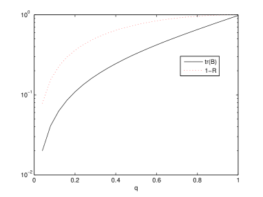
Figure 1: Trade-off in the BGA between $\operatorname{tr}(B)$ and $R$ as functions of $q$, for a complete graph with $N=30$.

Next, we focus on Abelian Cayley graphs.

Lemma 4.4

Consider the BGA algorithm and let the communication graph $\mathcal{G}$ be Abelian Cayley with degree $d$. Then, the MSA vector $\pi$ evolves as

$$\pi(t+1)=(C+T)\pi(t),$$ (19)

where the matrix

$$C=I-2\frac{q}{N}(L+L^{*})$$

is Cayley and $T$ is a matrix such that $\displaystyle T=\frac{q^{2}}{N}\tilde{T}$ where $\tilde{T}$ does not depend neither on $q$ nor explicitly on $N$ but only on $S$, and is such that the number of non-zero rows is at most $d^{2}$ and non-zero columns is at most $d^{2}-d+1$.

Proof: Using the fact that all matrices are Abelian Cayley, we obtain

$$\Delta(t+1)= \mathbb{E}[P(t)^{*}\Delta(t)P(t)]$$

$$= \Delta(t)-q\mathbb{E}[L(t)^{*}\Delta(t)]-q\mathbb{E}[\Delta(t)L(t)]+q^{2}\mathbb{E}[L(t)^{*}\Delta(t)L(t)]$$

$$= \left(I-\frac{q}{N}(L+L^{*})\right)\Delta(t)+q^{2}\frac{1}{N}\sum_{g\in G}\sum_{h:h-g\in S}\sum_{k:k-g\in S}(e_{g}e_{h}^{*}-e_{h}e_{h}^{*})\Delta(t)(e_{k}e_{g}^{*}-e_{k}e_{k}^{*})$$

Since $\pi(t)=\Delta(t)e^{0}$ (being $\Delta(t)$ symmetric for every $t$), we easily obtain from above that

$$\pi(t+1)= (I-q\frac{1}{N}(L+L^{*}))\pi(t)+\frac{1}{N}q^{2}\sum_{g\in G}\sum_{h:h-g\in S}\sum_{k:k-g\in S}\pi_{h-k}(t)(e_{g}e_{g}^{*}-e_{g}e_{k}^{*}-e_{h}e_{g}^{*}+e_{h}e_{k}^{*})e_{0}$$

$$= (I-q\frac{1}{N}(L+L^{*})\pi(t)+\frac{1}{N}q^{2}[\sum_{h:h\in S}\sum_{k:k\in S}\pi_{h-k}(t)(e_{0}-e_{h})+\sum_{g\in-S}\sum_{h:h-g\in S}\pi_{h}(t)(e_{h}-e_{g})]\,.$$

From this we immediately see that the non-zero elements of $\tilde{T}$ have row indices in $(S-S)\cup S$ and column indices in $S-S$. Hence the result follows.

 

Note that, in general, $C$ will not be a stochastic matrix since it may be negative on the diagonal, however for large enough $N$ (and $d$ fixed) it is surely a stochastic matrix. Note, moreover, that the entries of the matrix $T$ in (19) are proportional to $N^{-1}$ and, moreover, the number of the non-zero entries is upper bounded by $(1+d^{2})^{2}$, which does not depend on $N$. Hence, we expect that, as $N$ diverges, $T$ would become negligible, and the MSA would depend on the matrix $C$ only. This would imply the unbiasedness of the algorithm, because it is immediate to remark that the invariant vector of $C$ is $N^{-1}\mathbf{1}.$ This fact can be actually stated as the following result.

Theorem 4.5 (Unbiasedness of BGA)

Fix a finite $S\subseteq\mathbb{Z}^{d}\setminus\{0\}$ generating $\mathbb{Z}^{d}$ as a group. For every integer $n$, let $V_{n}=[-n,n]^{d}$ considered as the Abelian group $\mathbb{Z}_{2n+1}^{d}$ and let $\mathcal{G}^{(n)}$ be the Cayley Abelian graph generated by $S_{n}=S\cap[-n,n]^{d}$. On the sequence of $\mathcal{G}^{(n)}$ the BGA is asymptotically unbiased.

Proof: The idea is to apply the perturbation result Theorem 3.5 to the sequence of matrices $C^{*}$ and $(C+T)^{*}$. Notice that ${\mathcal{G}}_{C^{*}}=\mathcal{G}^{(n)}$ while ${\mathcal{G}}_{(C+T)^{*}}\supseteq\mathcal{G}^{(n)}$ by Lemma 3.4. Hence, ${\cal G}_{C^{*}}$ and ${\mathcal{G}}_{(C+T)^{*}}$ are both strongly connected. This also implies that the limit graph on $Z_{n}^{d}$ of the two sequences ${\mathcal{G}}_{C^{*}}$ and ${\mathcal{G}}_{(C+T)^{*}}$ both contain $\mathcal{G}^{(\infty)}$ which is simply the Abelian Cayley graph on $Z_{n}^{d}$ generated by $S$ which is strongly connected by the assumption made. Finally, notice that $C^{*}$ is Abelian Cayley, hence obviously weakly democratic, while Lemma 4.4 guarantees that $(C+T)^{*}$ is a finite perturbation of $C^{*}$ in the sense of Section 3.3. Hence also $(C+T)^{*}$ is weakly democratic. This yields, by (11),

$$\operatorname{tr}B=|N^{-1}-\pi^{\prime}_{0}|\leq N^{-1}+\pi^{\prime}_{0}\to 0.$$

 

The results about Cayley graphs can be made more specific in the following example.

Example 4.6 (Ring graph)

Note that in this case the Cayley graph is circulant. For the ring graph, Proposition 4.1 implies that, for $N$ large enough,

$$1-q\frac{8\pi^{2}}{N^{3}}\leq R\leq 1-q(1-q)\frac{8\pi^{2}}{N^{3}},$$

and namely ${R=1-\Theta(\frac{1}{N^{3}})}$. Specializing the proof of Lemma 4.4, the evolution of $\pi(t)$ can be written as

$$\pi_{j}(t+1)= \left(1-\frac{4q}{N}+\frac{q^{2}}{N}\pi^{A^{2}}_{j}\right)\pi_{j}(t)+2\left(\frac{q}{N}-\frac{q^{2}}{N}\pi^{A}_{j}\right)(\pi_{j-1}(t)+\pi_{j+1}(t))+\frac{q^{2}}{N}\left(2\pi_{0}(t)+\pi_{2}(t)+\pi_{-2}(t)\right)\delta_{0j},$$

that is $\pi(t+1)=(C+T)\pi(t)$, with

$$C=\operatorname{circ}{(1-\frac{4q}{N},2\frac{q}{N},0,\ldots,0,2\frac{q}{N})}$$

and

$$T=\frac{q^{2}}{N}\left(\begin{array}[]{cccccccc}4&0&1&0&\dots&0&1&0\\ -2&0&-2&0&\ldots&&\ldots&0\\ 0&0&1&0&\ldots&&\ldots&0\\ 0&\ldots&&&&&\ldots&0\\ 0&\ldots&&&&&\ldots&0\\ 0&\ldots&&&&&\ldots&0\\ 0&\ldots&&&\ldots&0&1&0\\ -2&0&\ldots&&\ldots&0&-2&0\\ \end{array}\right).$$

Thanks to these explicit formulas, we can numerically compute the rate and bias. Namely, about the rate we obtain that $\operatorname{esr}(C)<\operatorname{esr}(C+T)$, and $\operatorname{esr}(C+T)=1-\Theta(N^{-3})$. This means that the perturbation $T$ does not significantly affect the rate for large $N$. Moreover, since $\operatorname{esr}(C)=1-\Theta(N^{-3})$ and $\operatorname{esr}(C+T)-\operatorname{esr}(C)=1-\Theta(N^{-4})$ we argue that actually

$$R=1-q\frac{8\pi^{2}}{N^{3}}+O\left(\frac{1}{N^{4}}\right)\qquad\text{as $t\to\infty$}.$$

On the other hand, about the bias we obtain that $\operatorname{tr}{(B)}=\Theta(N^{-1})$. We can also numerically evaluate $B$ and $R$ as functions of $q$: these results are shown in Figure 2. Note that choosing $q$ we can trade off asymptotical error and convergence rate.  

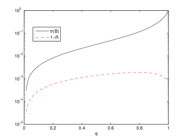
Figure 2: Trade-off in the BGA between $\operatorname{tr}{(B)}$ and $R$ for a ring graph with $N=30$.

Remark 4.1 (Pareto optimality)

Combining Examples 4.3 and 4.6, we obtain that $\operatorname{tr}B$ is proportional to $\frac{1-\sqrt{R}}{1+\sqrt{R}}\big{(}1-\frac{1}{N}\big{)}$ on a complete graph, and to $N^{3}(1-R)$ on a ring graph, considering the approximation for large $N$. In Figure 3 we plot $\operatorname{tr}B$ against $R$, for both graphs, up to a suitable scaling with respect to $N$. The fact that both curves are monotone decreasing highlights the fact that every value of $q$ is Pareto optimal, in the sense that one can not improve one of the two objectives without making the other worse.

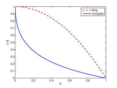
Figure 3: $\operatorname{tr}B$ as a function of $R$ on complete and ring graphs.

Example 4.7 (Random geometric graph)

In order to take into account the locality constraint on connectivity in real-world networks, several models of random geometric graphs have been proposed, as accounted in [20]. In this example we consider sequences of random geometric graphs, based on the following construction. For all $N\in\mathbb{N}$, we sample $N$ points $\{z_{i}\}_{i\in\mathbb{Z}_{N}}$ from a uniform distribution over a unit square $[0,1]^{2}$, and we draw an edge $(i,j)$ between nodes $i,j\in\mathbb{Z}_{N}$ when $\|z_{i}-z_{j}\|\leq 0.8\sqrt{\frac{\log{N}}{N}}.$ On these realizations we run the BGA algorithm until convergence is reached, up to a small tolerance threshold, and in this way we compute an approximation of $\lim_{t\to\infty}\beta(t).$ The results are plotted in Figure 4, in comparison with the analogous quantity on the complete and ring graph. It appears from simulations that, as $N$ diverges, $\beta$ is $\Theta(1)$ on the complete graph, whereas it is $\Theta(N^{-1})$ on the ring graph, and $\Theta(N^{-1/2})$ on the random geometric graph. These evidences are in accordance with the theoretical results, and suggest their extension to other families of geometric graphs.

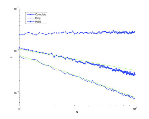
Figure 4: The plot shows the asymptotical bias $\beta$ as a function of $N$, computed by simulations on sequences of complete, random geometric, and ring graphs. Plotted values are the average over 1000 runs. See text for more information.

5 Broadcast with collisions

In this section we present a comprehensive analysis of the Collision Broadcast Gossip Algorithm, in terms of both rate of convergence and bias. After proving a general convergence result, we focus on complete graphs in Subsection 5.1, on Abelian Cayley graphs in Subsection 5.2, and finally on ring graphs in Subsection 5.3. Our main finding is that the performance of the CBGA, in terms of both speed and bias, is close to the BGA: in this sense we may claim the robustness of broadcast gossip algorithms to local interferences.

Proposition 5.1 (Convergence of CBGA algorithm)

Consider the CBGA algorithm. Let $\mathcal{G}$ be any connected graph, and $L$ its Laplacian matrix. Then,

$$\bar{P}=I-qp(1-p)^{D^{-}}L,$$ (20)

where $((1-p)^{D^{-}})_{ij}=(1-p)^{D^{-}_{ij}}$ for every $i$ and $j$. In particular, the CBGA algorithm achieves probabilistic consensus.

Proof: The probability of having at time $t$ a successful transmission from $v$ to $u$ is $\mathbb{P}[A_{uv}(t)=1]=p(1-p)^{d^{-}_{u}}A_{uv}$. Hence,

$$\mathbb{E}(A(t))=p(1-p)^{D^{-}}A\,.$$ (21)

Now,

$$\bar{P}=\mathbb{E}[P(t)] =\mathbb{E}[I+q(A(t)-D(t))]=I+qp(1-p)^{D^{-}}[A-{D^{-}}].$$

Note that $\mathcal{G}_{\bar{P}}$ is strongly connected: by Proposition 3.1, we can conclude the convergence of the CBGA.   

Remark: Formula (20) is simpler if the graph is $d$-regular, because in that case

$$\bar{P}=I-qp(1-p)^{d}L.$$ (22)

Denote by that $\lambda_{1}$ is the smallest nonzero eigenvalue of $L$. Then $\operatorname{esr}({\bar{P}})=1-qp(1-p)^{d}\lambda_{1}$, and this together with (5) and $[1-qp(1-p)^{d}\lambda_{1}]^{2}\geq 1-2qp(1-p)^{d}\lambda_{1}$ leads to

$$R\geq 1-2qp(1-p)^{d}\lambda_{1}$$ (23)

as a lower bound for the rate of convergence. As a function of $p$, this lower bound is minimal whenever $\mathbb{P}[A_{ij}(t)=1]$ is maximal, that is for $p$ equal to $p^{*}=\frac{1}{d+1}.$

Hence, natural questions are: is this bound tight? is $p^{*}$ the best choice to improve the convergence rate? The content of the next section will answer positively these questions for complete and ring graphs.

5.1 Complete graphs

A thorough analysis can be carried on for the complete graph.

Proposition 5.2 (Complete graph)

Let $x(t)$ evolve following the CBGA algorithm, and let $R$ and $B$ be defined by (4) and (7), respectively. Then,

$$R=1-q(2-q)Np(1-p)^{N-1}$$

$$B=\frac{q}{2-q}\frac{1}{N}(I-\frac{\mathbf{1}\mathbf{1}^{*}}{N}).$$

Namely, $\operatorname{tr}(B)=\frac{q}{2-q}\left(1-\frac{1}{N}\right)$ and then the CBGA is not asymptotically unbiased on the complete graph.

Proof: It is immediate that in the complete graph either one node communicates to every others, or no node communicates. In the latter case, $P(t)=I$. The former case, which has probability $Np(1-p)^{N-1}$, leads to $P(t)=P_{b}$, where $P_{b}=I+q\sum_{u\neq v}(e_{u}e_{v}^{*}-e_{u}e_{u}^{*})$ and $v$ is the realization of a random variable uniformly distributed over the nodes. Consequently, the analysis is quite close to the one of Example 4.3. We note that

$$\mathbb{E}[P_{b}]=I+q\frac{\mathbf{1}\mathbf{1}^{*}-NI}{N}$$

and that

$$\mathbb{E}[P(t)^{*}P(t)]= Np(1-p)^{N-1}\mathbb{E}[P_{b}^{*}P_{b}]+(1-Np(1-p)^{N-1})I$$

$$= Np(1-p)^{N-1}[I+2q\frac{\mathbf{1}\mathbf{1}^{*}-NI}{N}+q^{2}\left(\frac{N-1}{N}I-\frac{2}{N}(\mathbf{1}\mathbf{1}^{*}-I)+\frac{N-1}{N}I\right)]$$

$$+(1-Np(1-p)^{N-1})I$$

$$= Np(1-p)^{N-1}[I-2q(1-q)(I-\frac{\mathbf{1}\mathbf{1}^{*}}{N})]+(1-Np(1-p)^{N-1})I$$

$$= [1-2q(1-q)Np(1-p)^{N-1}]I+2q(1-q)Np(1-p)^{N-1}\frac{\mathbf{1}\mathbf{1}^{*}}{N}.$$

and

$$\mathbb{E}[P(t)^{*}\mathbf{1}\mathbf{1}^{*}P(t)]= Np(1-p)^{N-1}\big{[}\mathbf{1}\mathbf{1}^{*}+\frac{q^{2}}{N}\big{(}(N-1)^{2}I-2(N-1)(\mathbf{1}\mathbf{1}^{*}-I)$$

$$+(N-2)(\mathbf{1}\mathbf{1}^{*}-I)+(N-1)I\big{)}\big{]}+(1-Np(1-p)^{N-1})\mathbf{1}\mathbf{1}^{*}$$

$$= q^{2}N^{2}p(1-p)^{N-1}I+(1-q^{2}Np(1-p)^{N-1})\mathbf{1}\mathbf{1}^{*}.$$

This means that the application of $\mathcal{L}$ keeps invariant the subspaces generated by $I$ and $\mathbf{1}\mathbf{1}^{*}$, and the linear operator $\mathcal{L}$ can be represented by the matrix

$$\left(\begin{array}[]{cc}1-2q(1-q)Np(1-p)^{N-1}&q^{2}Np(1-p)^{N-1}\\ 2q(1-q)Np(1-p)^{N-1}&1-q^{2}Np(1-p)^{N-1}\\ \end{array}\right).$$

The eigenvalues of this matrix are $1$ and

$$R =1-q^{2}Np(1-p)^{N-1}-2q(1-q)Np(1-p)^{N-1}$$

$$=1-q(2-q)Np(1-p)^{N-1},$$

and the eigenspace relative to eigenvalue 1 is spanned by

$$qNp(1-p)^{N-1}\left(\begin{array}[]{c}q\\ 2(1-q)\\ \end{array}\right).$$

Since $E[\rho\rho^{*}]$ belongs to this eigenspace, and $\mathbf{1}^{*}E[\rho\rho^{*}]\mathbf{1}=1,$ we conclude that

$$B=E[\rho\rho^{*}]-N^{-2}\mathbf{1}\mathbf{1}^{*}=\frac{q}{2-q}\frac{1}{N}\big{(}I-\frac{\mathbf{1}\mathbf{1}^{*}}{N}\big{)}.$$

 

Some remarks are in order about the role of the parameters $p,q$ in the CBGA algorithm on the complete graph.

Remark 5.1 (Optimization)

The convergence rate $R$ as a function of $p$ is optimal for $p^{*}=1/N.$ The optimal value $R(p^{*})=1-q(2-q)(1-\frac{1}{N})^{N-1}$ is increasing in $N$ and tends to $1-q(2-q)\frac{1}{e}$ when $N$ goes to infinity. Instead, if we fix $p=\bar{p}$, $R(\bar{p})$ tends to 1 as $N\to\infty$. On the other hand, $B$ is the same as for the BGA in Example 4.3 and is independent of $p$.

From the design point of view, it is clear that $p$ has to be chosen equal to $N^{-1}$, optimizing the speed. Instead, choosing $q$ we trade off speed and asymptotic displacement: this trade-off is numerically investigated in Figure 5.

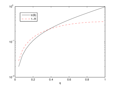
Figure 5: Trade-off in the CBGA between $\operatorname{tr}(B)$ and $R$ as functions of $q$, for a complete graph with $N=30$ and $p=1/N$.

5.2 Abelian Cayley graphs

In this subsection we consider the CBGA on Abelian Cayley graphs with bounded degree. The next result characterizes the mean square analysis of the algorithm.

Lemma 5.3

Consider the CBGA algorithm and let the communication graph $\mathcal{G}$ be Abelian Cayley with degree $d$. Then, the MSA vector $\pi$ evolves as

$$\pi(t+1)=(C+T)\pi(t),$$ (24)

where the matrix

$$C=(I-qp(1-p)^{d}L^{*})(I-qp(1-p)^{d}L)$$

is Cayley and $T$ is a matrix whose entries do not depend on $N$ and such that the number of non-zero rows is at most $d^{2}(d+1)^{2}$ and non-zero columns is at most $d^{2}$.

Proof: Using commutativity of Abelian Cayley matrices and (21), we obtain that

$$\Delta(t+1)=(I-qp(1-p)^{d}(L+L^{*}))\Delta(t)+q^{2}\mathbb{E}[L(t)^{*}\Delta(t)L(t)]$$ (25)

Passing to the generating vector,

$$\pi(t+1)=(I-qp(1-p)^{d}(L+L^{*}))\pi(t)+q^{2}f(\pi(t)$$ (26)

where

$$f(\pi(t)):=\mathbb{E}[L(t)^{*}\Delta(t)L(t)]e^{0}=\underbrace{\mathbb{E}[L(t)]^{*}\Delta(t)\mathbb{E}[L(t)]e^{0}}_{=:f_{1}(\pi(t))}+\underbrace{\mathbb{E}[L(t)^{*}\Delta(t)L(t)]e^{0}-\mathbb{E}[L(t)]^{*}\Delta(t)\mathbb{E}[L(t)]e^{0}}_{=:f_{2}(\pi(t))}$$

Now,

$$f_{1}(\pi(t))=p^{2}(1-p)^{2d}L^{*}L\pi(t)$$ (27)

and

$$\begin{array}[]{rcl}[f_{2}(\pi(t))]_{l}&=&\sum_{hk}\left[\mathbb{E}[L(t)_{hl}L(t)_{k0}\right]-\mathbb{E}[L(t)_{hl}]\mathbb{E}[L(t)_{k0}]\pi(t)_{h-k}\\[10.0pt] &=&\sum_{tk}\left[\mathbb{E}[L(t)_{k+t,l}L(t){k0}\right]-\mathbb{E}[L(t)_{k+t,l}]\mathbb{E}[L(t){k0}]\pi(t)_{t}\end{array}$$ (28)

Notice now that, by the way the model has been defined, we have that $A_{ij}(t)$ and $A_{hk}(t)$ are independent whenever $N^{-}(i)\cap N^{-}(h)=\emptyset$ or equivalently $i-h\not\in S-S$. In this case, also $L_{ij}(t)$ and $L_{hk}(t)$ are independent. Therefore, the double summation in (28), can be restricted to $k\in S\cup\{0\}$ and $t\in S-S$. Consequently, the values of $l$ for which $[f_{2}(\pi(t))]_{l}\neq 0$ can be restricted to $(S\cup\{0\})+S-S-(S\cup\{0\})$. Plugging (27) inside (26) and using the information on the structure of $f_{2}(\pi(t))$ obtained above, the result follows.

 

Thanks to Lemma 5.3, we can argue a result analogous to Theorem 4.5.

Theorem 5.4 (Unbiasedness of CBGA)

Fix a finite $S\subseteq\mathbb{Z}^{d}\setminus\{0\}$ generating $\mathbb{Z}^{d}$ as a group. For every integer $n$, let $V_{n}=[-n,n]^{d}$ considered as the Abelian group $\mathbb{Z}_{2n+1}^{d}$ and let $\mathcal{G}^{(n)}$ be the Cayley Abelian graph generated by $S_{n}=S\cap[-n,n]^{d}$. On the sequence of $\mathcal{G}^{(n)}$ the CBGA is asymptotically unbiased.

Proof: The idea is to apply the perturbation result Theorem 3.5to the sequence of matrices $C^{*}$ and $(C+T)^{*}$. Notice that ${\cal G}_{C^{*}}=\mathcal{G}_{A+A^{*}+A^{*}A}\supseteq\mathcal{G}^{(n)}$ while ${\cal G}_{(C+T)^{*}}\supseteq\mathcal{G}^{(n)}$ by Lemma 3.4. Hence, ${\cal G}_{C^{*}}$ and ${\cal G}_{(C+T)^{*}}$ are both strongly connected. As in the proof of Theorem 4.5 this also implies that the limit graph on $Z_{n}^{d}$ of the two sequences ${\cal G}_{C^{*}}$ and ${\cal G}_{(C+T)^{*}}$ are also strongly connected. Finally, notice that $C^{*}$ is Cayley Abelian, hence obviously weakly democratic, while Lemma 4.4 guarantees that $(C+T)^{*}$ is a finite perturbation of $C^{*}$ in the sense of Section 3.3. Hence also $(C+T)^{*}$ is weakly democratic. This yields

$$\operatorname{tr}B=|N^{-1}-\pi^{\prime}_{0}|\leq N^{-1}+\pi^{\prime}_{0}\to 0.$$

 

The form of $T$ depends on the graph, and is complicated to compute in general. To give an example, in the next subsection we shall compute $T$ for the ring graph.

5.3 Ring graphs

In this subsection, we specialize the results about about Cayley graphs to the case of ring graphs. In particular, we obtain tight bounds on its convergence rate. The following lemma can be proved on the lines of Lemma 5.3 by a direct computation, which we omit.

Lemma 5.5

Let $\mathcal{G}$ be a ring graph on $N\geq 9$ nodes. Let $C$ be the doubly stochastic symmetric circulant matrix $C=\operatorname{circ}([1-2k_{1}-2k_{2},k_{1},k_{2},0,\ldots,0,k_{2},k_{1}])$ with

$$k_{1}=2qp(1-p)^{2}(1-2qp(1-p)^{2})$$

$$k_{2}=q^{2}p^{2}(1-p)^{4},$$

and let

$$T=q^{2}p(1-p)^{2}\cdot$$

$$\left(\begin{array}[]{cccccccc}4-6p(1-p)^{2}&4p(1-p)^{2}&(1-p)^{3}&0&\ldots&(1-p)^{3}&4p(1-p)^{2}\\ 4p(1-p)^{2}-2&(1-6(1-p)^{2})p&2(2p-1)(1-p)^{2}&0&\ldots&0&-p(1-p)^{2}\\ -p(1-p)^{2}&4p(1-p)^{2}-2p&(1-p)(1-6p(1-p))&0&\ldots&0&0\\ 0&(1-(1-p)^{2})p&-2p(1-p)(2p-1)&0&\ldots&0&0\\ 0&0&p^{2}(1-p)&0&\ldots&0&0\\ 0&0&0&0&\ldots&0&0\\ \ldots&\ldots&\ldots&\ldots&\ldots&\ldots&\ldots\\ 0&0&0&0&\ldots&p^{2}(1-p)&0\\ 0&0&0&0&\ldots&-2p(1-p)(2p-1)&(1-(1-p)^{2})p\\ -p(1-p)^{2}&0&0&0&\ldots&(1-p)(1-6p(1-p))&4p(1-p)^{2}-2p\\ 4p(1-p)^{2}-2&-p(1-p)^{2}&0&0&\ldots&2(1-p)^{2}(2p-1)&(1-6(1-p)^{2})p\\ \end{array}\right)$$

Then, the MSA vector evolves as $\pi(t+1)=(C+T)\pi(t).$

Numerical computations based on Lemma 5.5 show that $\operatorname{tr}(B)=\Theta(N^{-1})$, that is the asymptotical error has the same dependence on $N$ as for the BGA.

Next result is about the rate of convergence, and shows that the bound on the convergence rate based on $\bar{P}$ is tight for the ring graph.

Proposition 5.6 (Ring graph - Rate)

Given a ring graph and CBGA algorithm, we have

$$\bar{P} =I-qp(1-p)^{2}L;$$

$$\mathcal{L}(\Omega) =\Omega-2q(1-q)p(1-p)^{2}L-q^{2}p(1-p)^{2}N^{-1}L^{2}+q^{2}p(1-p)^{2}N^{-1}p\operatorname{circ}(\tau),$$

where

$$\tau=[2(p-2),6-4p+p^{2},-3(2-2p+p^{2}),2-4p+3p^{2},0,\ldots,0,2-4p+3p^{2},-3(2-2p+p^{2}),6-4p+p^{2}].$$

Namely,

$$1-qp(1-p)^{2}\frac{8\pi}{N^{2}}\leq R \leq 1-q(1-q)p(1-p)^{2}\frac{8\pi}{N^{2}}\qquad\text{ for $N$ large enough}.$$

Proof: Computing $\bar{P}$ is easy. In order to compute $\mathcal{L}(\Omega)$, we first compute, using Lemma 5.5,

$$\mathcal{L}(I)= \operatorname{circ}((C+T)(1,0,\ldots,0)^{*})$$

$$= \operatorname{circ}(1-2k_{1}-2k_{2}+q^{2}p(1-p)^{2}(4-6p(1-p)^{2}),k_{1}+q^{2}p(1-p)^{2}(4p(1-p)^{2}-2),$$

$$\qquad k_{2}-q^{2}p(1-p)^{2}p(1-p)^{2},0,\ldots,0,k_{2}-q^{2}p(1-p)^{2}p(1-p)^{2},$$

$$\qquad k_{1}+q^{2}p(1-p)^{2}(4p(1-p)^{2}-2))$$

$$= \operatorname{circ}(1-4q(1-q)p(1-p)^{2},2p(1-p)^{2}q(1-q),0,\ldots,0,2p(1-p)^{2}q(1-q))$$

$$= -2q(1-q)p(1-p)^{2}L,$$

and

$$\mathcal{L}(\mathbf{1}\mathbf{1}^{*})= \operatorname{circ}((C+T)\mathbf{1})=\mathbf{1}\mathbf{1}^{*}+\operatorname{circ}(T\mathbf{1}).$$

Then, by straightforward computations,

$$\mathcal{L}(\Omega)= \Omega-2q(1-q)p(1-p)^{2}L-\operatorname{circ}(T\mathbf{1})$$

$$= \Omega-2q(1-q)p(1-p)^{2}L-q^{2}p(1-p)^{2}N^{-1}L^{2}+q^{2}p^{2}(1-p)^{2}N^{-1}\operatorname{circ}(\tau),$$

provided we define $\tau$ as in the statement.

Note that $\tau^{*}\mathbf{1}=0$ and that the eigenvalues of the circulant matrix $\operatorname{circ}(\tau)$ are

$$\left\{\tau_{0}+2\sum_{i=1}^{4}\tau_{i}\cos{\left(\frac{2\pi}{N}il\right)}\right\}_{l\in\mathbb{Z}_{N}},$$

and those of $L$ are $\left\{2\left(1-\cos{\left(\frac{2\pi}{N}l\right)}\right)\right\}_{l\in\mathbb{Z}_{N}}.$ As a consequence, the eigenvalues of $\mathcal{L}(\Omega)$ are $\mu_{0}=0$, and

$$\mu_{l}= 1+2p(1-p)^{2}[-2q(1-q)-3q^{2}N^{-1}+\tau_{0}q^{2}pN^{-1}]$$

$$+2p(1-p)^{2}[2q(1-q)+4q^{2}N^{-1}+\tau_{1}q^{2}pN^{-1}]\cos{\left(\frac{2\pi}{N}l\right)}+2q^{2}p(1-p)^{2}N^{-1}[\tau_{2}p-1]\cos{\left(\frac{4\pi}{N}l\right)}$$

$$+2\tau_{3}q^{2}p^{2}(1-p)^{2}N^{-1}\cos{\left(\frac{6\pi}{N}l\right)}+2\tau_{4}q^{2}p^{2}(1-p)^{2}N^{-1}\cos{\left(\frac{8\pi}{N}l\right)},$$

for $l=1,\ldots,N-1.$ Because of the $N^{-1}$ factors, we have that, as $N\to\infty$,

$$\mu_{l}=1-4q(1-q)p(1-p)^{2}\frac{2\pi^{2}l^{2}}{N^{2}}+o\left(\frac{l^{2}}{N^{2}}\right).$$

Then, for $N$ large enough,

$$\operatorname{esr}\mathcal{L}(\Omega)=\max_{l\in\mathbb{Z}_{N}\setminus\{0\}}\mu_{l}=1-8q(1-q)p(1-p)^{2}\frac{\pi^{2}}{N^{2}}+o\left(\frac{1}{N^{2}}\right).$$

Finally, the bound on the rate follows from (5).   

Remark 5.2

The speed of convergence for the Collision Broadcasting Gossip is one order faster than the Broadcasting Gossip. This is not surprising, since in the former case the average number of activated nodes per round is $Np$, instead of $1$.

Remark 5.3 (Rate Optimization)

Remarkably, for $N$ large enough both the upper and the lower bound on the rate show the same dependence on $p$. Thus, they can be simultaneously optimized by taking $p^{*}=1/3.$ The behavior for large $N$ can also be investigated by numerical computations, showing that $\operatorname{esr}(C)<\operatorname{esr}(C+T)$, and $\operatorname{esr}(C+T)=1-\Theta(N^{-2})$. This means that the perturbation $T$ does not significantly affect the rate for large $N$. Moreover, since $\operatorname{esr}(C)=1-\Theta(N^{-2})$ and $\operatorname{esr}(C+T)-\operatorname{esr}(C)=1-\Theta(N^{-3})$, we argue that actually

$$R=1-qp(1-p)^{2}\frac{8\pi^{2}}{N^{2}}+O\left(\frac{1}{N^{3}}\right).$$

This is reminiscent of a similar observation about the BGA algorithm in Remark 4.6.

We can also numerically evaluate $B$ and $R$ as functions of $p$ and $q$: these results are shown in Figure 6. Note that the asymptotical error does not depend significantly on $p$: this implies, from the design point of view, that $p$ can be chosen equal to $p^{*}=1/3$, optimizing the convergence rate. Instead, choosing $q$ we can trade off asymptotical error and convergence rate.

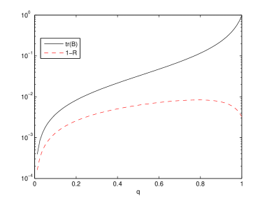
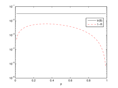
Figure 6: Dependence in the CBGA of $\operatorname{tr}{(B)}$ and $R$ for the ring graph. Left plot assumes $N=30$, $p=1/3$, right plot assumes $N=30$, $q=1/2$.

6 Conclusion

This paper has been devoted to study gossip algorithm for the estimation of averages, based on iterated broadcasting of current estimates, focusing on their capability of providing an unbiased estimation. In this framework, we presented a novel broadcast gossip algorithm, dealing with interference in communications, whose impact is studied in the paper. Our results, obtained under specific symmetry assumptions about the network topology, allow to conjecture an interesting picture of the performance of broadcast gossip algorithms on real world networks, in terms of achievable precision and robustness to interference. Interferences have a negative effect on the rate of convergence, which can be minimized by a suitable choice of the broadcasting probability $p$. As known for static consensus algorithms based on diffusion, the rate degrades on large locally connected graphs. Instead, interferences have minimal effect on the asymptotical error, which depends on the network topology: on large highly connected graphs, the algorithms provide biased estimations, whereas on locally connected graphs the estimation bias goes to zero as the network grows larger.

A better understanding of the role of the network topology in the trade-off between speed and achievable precision might come from the following extensions of our work. In this paper two simultaneous technical assumptions have been made: the graphs are Abelian Cayley, thus in particular vertex-transitive, and each node broadcasts with the same probability. Future work should consider non-vertex-transitive networks of nodes with non-uniform broadcasting probabilities. Furthermore, it seems interesting to study the performance of the algorithms on families of expander graphs and small-world networks, which ensure a good scaling of the rate of convergence, while keeping the degree of nodes bounded.

Acknowledgements: The authors wish to thank Sandro Zampieri for many fruitful discussions on the issues studied in this paper.

References

- [1] N. Abramson. Development of the ALOHANET. IEEE Transactions on Information Theory, 31(2):119–123, 1985.
- [2] T. C. Aysal, A. D. Sarwate, and A. G. Dimakis. Reaching consensus in wireless networks with probabilistic broadcast. In Allerton Conf. on Communications, Control and Computing, Allerton, IL, USA, September 2009.
- [3] T. C. Aysal, M. E. Yildiz, A. D. Sarwate, and A. Scaglione. Broadcast gossip algorithms for consensus. IEEE Transactions on Signal Processing, 57(7):2748–2761, 2009.
- [4] L. Babai. Spectra of Cayley graphs. J. Combin. Theory Ser. B, 27(2):180–189, 1979.
- [5] F. Benezit, A. G. Dimakis, P. Thiran, and M. Vetterli. Gossip along the way: Order-optimal consensus through randomized path averaging. In Allerton Conf. on Communications, Control and Computing, Monticello, IL, US, Sep 2007.
- [6] S. Boyd, A. Ghosh, B. Prabhakar, and D. Shah. Randomized gossip algorithms. IEEE Transactions on Information Theory, 52(6):2508–2530, 2006.
- [7] R. Carli, A. Chiuso, L. Schenato, and S. Zampieri. A PI consensus controller for networked clocks synchronization. In IFAC World Congress, pages 10289–10294, Seoul, Korea, July 2008.
- [8] R. Carli, F. Garin, and S. Zampieri. Quadratic indices for the analysis of consensus algorithms. In 4th Information Theory and Applications Workshop, San Diego, CA, February 2009.
- [9] G. Chockler, M. Demirbas, S. Gilbert, N. Lynch, C. Newport, and T. Nolte. Consensus and collision detectors in radio networks. Distributed Computing, 21(1):55–84, 2008.
- [10] P. Denantes, F. Benezit, P. Thiran, and M. Vetterli. Which distributed averaging algorithm should I choose for my sensor network? In IEEE Conference on Computer Communications (INFOCOM), pages 986–994, April 2008.
- [11] P. Diaconis and L. Saloff-Coste. Comparison theorems for reversible Markov chains. The Annals of Applied Probability, 3(3):696–730, 1993.
- [12] A. G. Dimakis, A. D. Sarwate, and M. J. Wainwright. Geographic gossip: Efficient averaging for sensor networks. IEEE Transactions on Signal Processing, 56(3):1205–1216, 2008.
- [13] O. Dousse, F. Baccelli, and P. Thiran. Impact of interferences on connectivity in Ad Hoc Networks. IEEE-ACM Transactions on Networking, 13(2):425–436, 2005.
- [14] O. Dousse, M. Franceschetti, N. Macris, R. Meester, and P. Thiran. Percolation in the signal to interference ratio graph. Journal of Applied Probability, 43(2):552–562, 2006.
- [15] F. Fagnani and J.-C. Delvenne. Democracy in Markov chains and its preservation under local perturbations. In IEEE Conf. on Decision and Control, 2010. Submitted.
- [16] F. Fagnani and S. Zampieri. Randomized consensus algorithms over large scale networks. In Information Theory and Applications Workshop, San Diego, CA, 2007.
- [17] F. Fagnani and S. Zampieri. Randomized consensus algorithms over large scale networks. IEEE Journal on Selected Areas in Communications, 26(4):634–649, 2008.
- [18] F. Fagnani and S. Zampieri. Average consensus with packet drop communication. SIAM Journal on Control and Optimization, 48(1):102–133, 2009.
- [19] J. A. Fill. Eigenvalue bounds on convergence to stationarity for nonreversible Markov chains, with an application to the exclusion process. The Annals of Applied Probability, 1(1):62–87, 1991.
- [20] M. Franceschetti and R. Meester. Random networks for communication. Cambridge University Press, 2007.
- [21] F. Garin and S. Zampieri. Performance of consensus algorithms in large-scale distributed estimation. In European Control Conference, Budapest, Hungary, August 2009.
- [22] Y. W. Hong and A. Scaglione. Energy-efficient broadcasting with cooperative transmission in wireless sensor networks. IEEE Transactions on Wireless Communications, 5(10):2844–2855, 2006.
- [23] D. Kempe, A. Dobra, and J. Gehrke. Gossip-based computation of aggregate information. In IEEE Symposium on Foundations of Computer Science, pages 482–491, Washington, DC, October 2003.
- [24] S. Kirti, A. Scaglione, and R. J. Thomas. A scalable wireless communication architecture for average consensus. In IEEE Conf. on Decision and Control, pages 32–37, New Orleans, LA, December 2007.
- [25] Q. Li and D. Rus. Global clock syncronization in sensor networks. IEEE Transactions on Computers, 55(2):214– 226, 2006.
- [26] D. Mosk-Aoyama and D. Shah. Fast distributed algorithms for computing separable functions. IEEE Transactions on Information Theory, 54(7):2997–3007, 2008.
- [27] B. Nazer, A. G. Dimakis, and M. Gastpar. Local interference can accelerate gossip algorithms. In Allerton Conf. on Communications, Control and Computing, Allerton, IL, USA, September 2008.
- [28] S. Rai. The spectrum of a random geometric graph is concentrated. Journal of Theoretical Probability, 20(2):119–132, 2007.
- [29] B. Recht and R. D’Andrea. Distributed control of systems over discrete groups. IEEE Transactions on Automatic Control, 49(9):1446–1452, 2004.
- [30] V. Saligrama, M. Alanyali, and O. Savas. Distributed detection in sensor networks with packet losses and finite capacity links. IEEE Transactions on Signal Processing, 54(11):4118–4132, 2006.
- [31] A. Terras. Fourier analysis on finite groups and applications, volume 43 of London Mathematical Society Student Texts. Cambridge University Press, Cambridge Ma, 1999.