Anomalous variance in the WMAP data and Galactic Foreground residuals
Abstract
A previous work (Monteserín et al., 2008) estimated the CMB variance from the three-year WMAP data, finding a lower value than expected from Gaussian simulations using the WMAP best-fit cosmological model. We repeat the analysis on the five-year WMAP data using a new estimator with lower bias and variance. Our results confirm this anomaly at higher significance, namely with a -value of . We perform the analysis using different exclusion masks, showing that a particular region of the sky near the Galactic plane shows a higher variance than of the simulations whereas the rest of the sky has a lower variance than of the simulations. The relative difference in variance between both regions is bigger than in of the simulations. This anisotropic distribution of power seems to be causing the anomaly since the model assumes isotropy. Furthermore, this region has a clear frequency dependence between 41GHz and 61GHz or 94GHz suggesting that Galactic foreground residuals could be responsible for the anomaly. Moreover, removing the quadrupole and the octopole from data and simulations the anomaly disappears. The variance anomaly and the previously reported quadrupole and octopole alignment seem therefore to be related and could have a common origin. We discuss different possible causes and Galactic foreground residuals seem to be the most likely one. These residuals would affect the estimation of the angular power spectrum from the WMAP data, which is used to generate Gaussian simulations, giving rise to an inconsistency between the estimated and expected CMB variance. If the presence of residuals is confirmed, the estimation of the cosmological parameters could be affected.
keywords:
methods: data analysis - methods: statistical - cosmic microwave background1 Introduction
The Cosmic Microwave Background (CMB) is the most ancient image of the Universe. This image can reveal valuable information on the origin and evolution of the Universe. Many observations in different cosmological fields tend to support the concordance, standard inflationary model. This model predicts the temperature anisotropies of the CMB to represent a Gaussian and isotropic random field on the sphere, whereas non-standard models, such as topological defect models, predict departures from isotropy and/or Gaussianity.
The Wilkinson Microwave Anisotropy Probe (WMAP) satellite, provided the first all-sky, high resolution map (Bennett et al., 2003) of the CMB anisotropies. In the past years, many authors claimed to have found anomalies in the WMAP data. Some of them could be affected by a posteriori statistics but the list of anomalies is too long to be ignored without worry. Some of these anomalies are, asymmetry between ecliptic hemispheres (Eriksen et al., 2004; Hansen et al., 2004; Eriksen et al., 2004; Hansen et al., 2004; Eriksen et al., 2005; Donoghue & Donoghue, 2005; Land & Magueijo, 2005; Bernui et al., 2007; Eriksen et al., 2007; Bernui, 2009; Hoftuft et al., 2009; Pietrobon et al., 2010; Vielva & Sanz, 2010; Cayón, 2010); anomalous quadrupole-octupole alignment (Bielewicz et al., 2004; Copi et al., 2004; de Oliveira-Costa et al., 2004; Schwarz et al., 2004; Bielewicz et al., 2005; Abramo et al., 2006; Copi et al., 2006, 2007; Gruppuso & Burigana, 2009; Frommert & Enßlin, 2010); unexpected alignment of CMB structures towards the Ecliptic poles (Wiaux et al., 2006; Vielva et al., 2007); a prominent cold spot in the southern Galactic hemisphere (Vielva et al., 2004; Mukherjee & Wang, 2004; Cruz et al., 2005, 2006; Cruz et al., 2007a; Cruz et al., 2007b, 2008; McEwen et al., 2005; Cayón et al., 2005; Räth et al., 2007; Wiaux et al., 2008; Gurzadyan & Kocharyan, 2008; Pietrobon et al., 2008; Gurzadyan et al., 2009; Rossmanith et al., 2009).
These anomalies arise after using very sophisticated statistical methods. However, a very simple analysis already reveals some anomalies. Monteserín et al. (2008) estimated the CMB variance of the 3–year WMAP data and compared it to the values obtained from Gaussian simulations. The -value of the variance was . They confirmed this result by comparing with an analytic formula derived in Cayon et al. (1991). An analysis of the two ecliptic hemispheres revealed that the anomaly was mainly due to the low variance of the Northern ecliptic hemisphere. Similar results were found in Larson & Wandelt (2004) and Ayaita et al. (2009), analysing spot abundances.
Here we propose a new method to estimate the CMB variance from data with anisotropic noise. In section 2 we review the WMAP data and exclusion masks we use. We compare the new method to the one used in Monteserín et al. (2008) in section 3 and apply it to the 5–year WMAP data in section 4. Finally we present the conclusions of this paper in section 5.
2 WMAP data and exclusion masks
The WMAP team (Hinshaw et al., 2009) provides foreground-reduced maps for the Q (41 GHz), V (61 GHz), and W (94 GHz) bands. We use the WMAP foreground cleaned VW combined map:
| (1) |
where gives the position in the sky and the index stands for the 6 differencing assemblies of the V and W bands, namely V1, V2 for the V band and W1, W2, W3 and W4 for the W band. These are the data recommended for cosmological analyses, since their Galactic foreground contamination should be low. The noise weight is defined as:
| (2) |
where is the noise dispersion per observation for each differencing assembly and is the number of observations made by the receiver at the position in the sky .
Although the data are provided at a HEALPix111http://healpix.jpl.nasa.gov (Górski et al., 2005) resolution of , we degrade the data to since the smallest scales are dominated by noise. In addition, in order to avoid the strong contamination present at the Galactic plane and the emission coming from bright extragalactic point sources, we will apply different exclusion masks.
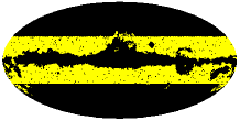
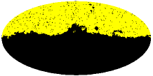
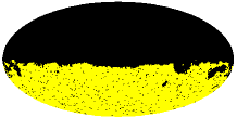
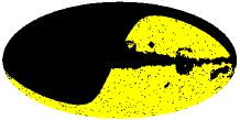
The WMAP team provides the kq85 and kq75 masks which leave approximately and of the sky unmasked. We construct two more masks by applying an additional and degrees Galactic latitude cut to the kq75 mask. Hereafter we will call these masks gc30 and gc40 respectively. These four masks are shown in Figure 1
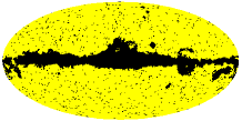
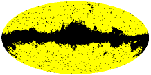


In our Galactic foreground analysis we build the gp33 and gp10 masks which admit only some pixels near the Galactic plane. The description of these masks is given in section 4.
The simulations are generated from the best fit angular power spectrum estimated from the data by the WMAP team. Note that the kq85 mask is used in the angular power spectrum estimation (Nolta et al., 2009). Isotropy and Gaussianity is assumed and the beam and noise properties are taken into account.
Note that the kp0 and kp2 masks given in the 3–year WMAP data release used in Monteserín et al. (2008), are analogous to the kq75 and kq85 masks but slightly different.
3 CMB variance estimation
Assuming that the foreground contamination has been totally removed, our data, , consist of two components, namely CMB, , and instrumental noise, .
| (3) |
The standard cosmological model predicts to represent an isotropic Gaussian random field. Hence, the CMB variance, , is constant for any position of the sky, , according to that model. Therefore
| (4) |
On the contrary, the noise is Gaussian, uncorrelated, but anisotropic. Hence the noise variance depends on the position on the sky, , but it can be calculated since the number of observations per pixel is known
| (5) |
Note that the correlated WMAP noise was shown to be negligible in section 4.2 of Monteserín et al. (2008). The aim of the present paper is to estimate , comparing the obtained value to that of Gaussian simulations and checking the isotropy of the CMB. We use a new estimator but let us review first the estimator used in Monteserín et al. (2008).
3.1 The minimum Kolmogorov-Smirnov distance estimator
The normalised CMB temperature is given by
| (6) |
According to the description given above, has a normal distribution:
| (7) |
In order to estimate the CMB variance, we replace by , which we allow to vary in a sufficiently large range. In this manner we can find the value which minimizes the Kolmogorov-Smirnov distance to a normalised Gaussian. This value is our estimate for . Hence we can write the minimum Kolmogorov-Smirnov estimator (hereafter MKS estimator) as:
| (8) |
where is the Cumulative distribution function of a standard normal and is the empirical distribution function for the normalised temperature.
3.2 The unit variance estimator
Here we propose an alternative way of estimating . We replace by a set of values varying in a sufficiently large range and find the value where the variance of the normalised map, is closer to unity. This value of is the estimated :
| (9) |
Let us check how this unit variance estimator (hereafter UV estimator) performs compared to the MKS estimator.
3.3 Comparing both estimators
Two estimators can be compared in terms of their mean squared error, which can be written as the sum of the variance and the squared bias. For an estimator trying to estimate the true value we have that the mean squared error reads:
| (10) |
where is the bias:
| (11) |
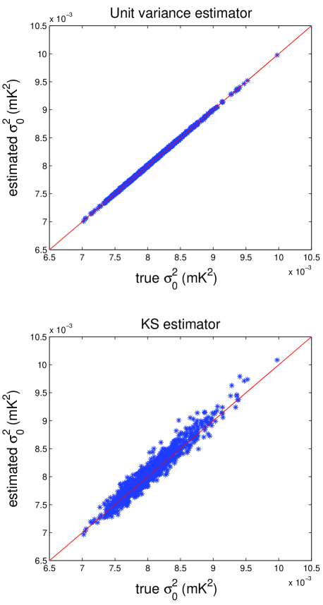
Since we only have one sky we estimate the mean squared error, variance and bias using simulations. Each simulation has a different , which can be calculated before adding the noise. The estimation of this quantity, , is then obtained applying the estimator to the simulation including the noise. Hence we take and . Note that corresponds to the distance of each dot to the red line in Figure 2. We apply the MKS and UV estimators to simulations using the kq75 mask. The results are shown in Table 1. The UV estimator performs better due to its lower bias and variance.
| Estimator | Mean Squared Error () | Bias () | Variance of the estimator () |
|---|---|---|---|
| UV | |||
| MKS |
Since we have found that the UV estimator performs better than the MKS one used in Monteserín et al. (2008), let us repeat the variance analysis with the new tool.
4 The Analysis
Applying the UV estimator to the WMAP foreground cleaned VW combined map we find which compared to simulations gives a -value of . The kq75 exclusion mask was used in this analysis. This -value is much lower than the one found in Monteserín et al. (2008) using the 3–year QVW combined map, masked with the 3–year kp0 mask.
The significance of the anomaly is high. No a posteriori choices have been made since the WMAP foreground cleaned VW combined map and the kq75 mask are recommended by the WMAP team for such analyses.
However the cause of the anomaly is unknown. In the following subsections we perform a number of follow-up tests to further investigate its possible origin, but these a posteriori tests are not valid to establish the significance of the anomaly. To make this clear, we will not consider the lower tail probabilities of the follow-up tests as -values.
Let us start applying different exclusion masks to analyse the possible cause of the anomaly.
4.1 Applying different exclusion masks
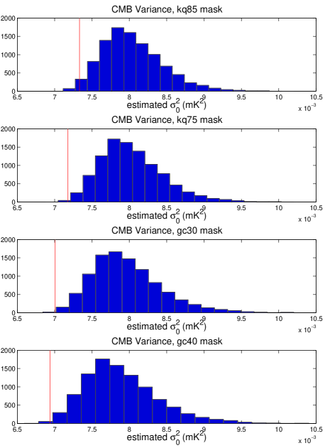
In Table 2 we list the results for the kq85, kp0, kq75, gc30 and gc40 masks in increasing order of masked pixels (see section 2 for the definition of the masks). The corresponding histograms are shown in Figure 3. The three year kp0 exclusion mask used in Monteserín et al. (2008) excluded less pixels than the kq75 mask used here and that does change in some extent the significance as can be seen in Table 2. Note that the lower tail probability decreases as the mask grows reaching its minimum at the gc30 mask and increases slightly for the gc40 mask.
| Mask | Sky Fraction Admitted (%) | Estimated Variance () | lower tail probability |
|---|---|---|---|
| kq85 | 81 | ||
| kp0 | 76 | ||
| kq75 | 71 | ||
| gc30 | 48 | ||
| gc40 | 34 |
The estimation of the variance and hence the variation of the lower tail probability is affected by the efficiency of the estimator. If we assume that the low variance was intrinsic to the all-sky CMB data, we would expect the lower tail probability to have its lowest value for the smallest mask (i.e. kq85) since the variance of the estimator is higher when less pixels are taken into account. Applying the UV estimator to simulations using the kq75 and gc40 masks, we find that the m.s.e of the estimator is higher for the gc40 mask respect to the kq75 one. The estimation is worse since less pixels are used. This has to be the reason for the higher lower tail probability for the gc40 mask compared to the gc30 one. Note that the histograms in Figure 3 are broader for bigger masks due to this effect.
However increasing the admitted fraction of the sky from the gc30 to the kq85 mask the lower tail probability grows instead of decreasing, hence this can not be due to estimator efficiency. This trend rather suggests a higher variance in the data near the Galactic plane, which could perhaps be due to Galactic foregrounds. Before further investigating this result, let us analyse the ecliptic hemispheres separately as was done in Monteserín et al. (2008).
4.2 Hemispherical analysis
Monteserín et al. (2008) found that the significance of the low variance was higher in the northern ecliptic hemisphere. Therefore we also analyse both ecliptic hemispheres separately, finding the same result but again with increased significance. Applying the kq85 mask, the northern ecliptic hemisphere shows a lower tail probability of while the southern one is compatible with the simulations (lower tail probability ). A similar result is found analysing Galactic, instead of ecliptic hemispheres. We find a lower tail probability of for the Galactic north and for the Galactic south (see Table 3).
4.3 Localising the anomalous region
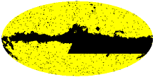
The most significant lower tail probability in Table 2 is obtained for the gc30 case. Therefore the pixels excluded by the gc30 mask seem to have a high variance. In order to study these pixels we build a complementary mask which admits only the pixels between the kq85 mask and the gc30 one (i.e. all the pixels not excluded by the kq85 mask but excluded by the gc30 one, see Figure 4). We call this mask gp33 since the admitted fraction of the sky is about and is located near the Galactic plane. The first two lines in Table 3 show the result obtained for the gp33 mask compared to the gc30 one. The gp33 result is compatible with the simulations and completely different from those found in Table 2. In the previous subsection we analysed separately Galactic and ecliptic hemispheres. The results were similar to those obtained when studying the complementary regions allowed by the gp33 and gc30 masks as we show in rows 3 to 6 in Table 3.



| Mask | Sky Fraction Admitted (%) | Estimated Variance () | lower tail probability |
|---|---|---|---|
| gc30 | 48 | ||
| gp33 | 33 | ||
| galN | 40 | ||
| galS | 41 | ||
| eclN | 41 | ||
| eclS | 40 | ||
| kq80 | 72 | ||
| gp10 | 9 |
Putting these three results together, it is clear that the intersection of the three high-variance regions (Galactic and ecliptic south, and gp33) could have an even higher variance. This intersection, i.e. the region of the sky admitted by all three masks, represents about of the sky. In order to study this region we build the gp10 mask admitting this small fraction of the sky and its complementary mask which we call kq80. In Figure 5 we show the Mollweide projection of these two masks applied to the WMAP VW combined map.
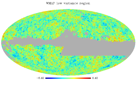
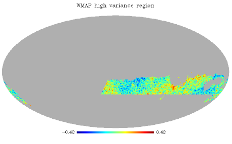
The estimated variances for these masks are listed in the last two lines of Table 3. The gp10 region shows an anomalously high variance, whereas the kq80 region presents an anomalously low variance. The histograms corresponding to Table 3 are plotted in Figure 6.
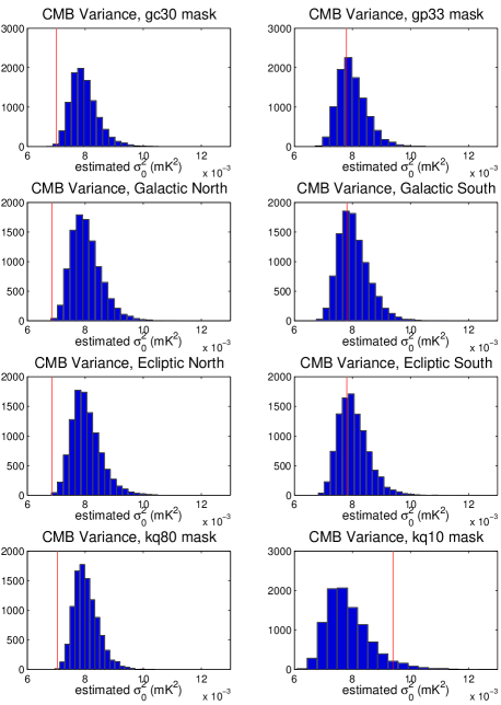
The relative difference of estimated variances between the WMAP gp10 and kq80 regions, is bigger than in of the simulations. Therefore, the different variance between the region near the Galactic plane and the rest of the sky seems to be violating the cosmological principle of isotropy and could be the cause of the anomalous variance. Isotropy is one of the key assumptions made to estimate the angular power spectrum (Nolta et al., 2009) and to generate the simulations. Let us recall the process we follow in this analysis. We use the best fit estimated from the data to generate Gaussian and isotropic simulations, and then we compare the variance of the simulations again to the data.
Since the kq85 mask is used for estimating the (Nolta et al., 2009) and there is an excess of power in the gp10 region, the isotropic simulations will have an excess of variance in the complementary kq80 region when compared to the data.
Hence the anomaly could not be due to an isotropic low variance of the data over the whole sky, but rather to an anisotropic power distribution.
The high variance in the Galactic plane region is a clear hint for Galactic foreground contamination, since adding any two independent emissions ends up in an increase of the variance. However we would need some other support for the Galactic foreground hypothesis, since the anisotropic variance distribution could be casual. Contaminating Galactic foregrounds such as synchrotron, free-free and Galactic dust emission show a strong frequency dependence. Therefore, a frequency dependence of the variance in the gp10 region would be proving the foreground hypothesis right.
4.4 Individual frequency bands
Here we perform the analysis on the Q (41 GHz), V (61 GHz) and W (94 GHz) frequency bands separately. We compare the estimated variance to simulations for each band.
We find a slight frequency dependence of the lower tail probability when using the gp10 mask but the significance remains almost unchanged using the kq80 one. The lower tail probabilities for the Q, V and W bands are , and respectively, using the kq80 mask; and , and applying the gp10 mask.
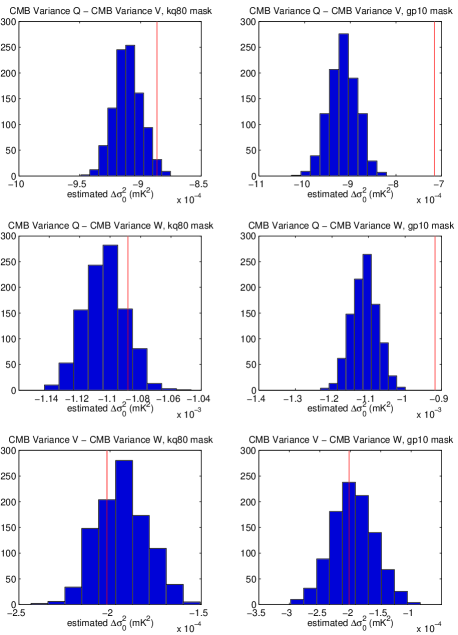
In order to check whether the frequency dependence of the variance is significant, we calculate the difference of the estimated variance between different bands, and compare their histograms to the data in Figure 7.
The gp10 variance differences including the Q band data, show a very high frequency dependende. This result indicates the presence of some foreground residuals near the Galactic plane in the Q band. The V and W bands which are the cosmological bands, do not show any anomalous frequency dependence, but the Q band result and the anomalously high variance make this region highly suspicious of being contaminated. The combination of dust and synchrotron or free-free emission could perhaps give a flat frequency dependence at the V and W frequencies. Moreover an artifact of the foreground cleaning process could be affecting the pixels in this region.
The excess of variance near the Galactic plane could be related to other, previously reported anomalies. For instance, many authors (see introduction) reported an anomalous quadrupole-octopole alignment in a direction near the Galactic plane.
4.5 Subtracting Quadrupole and Octopole
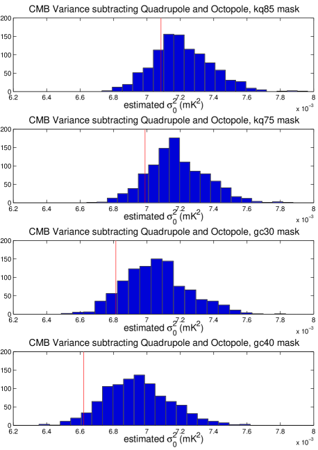
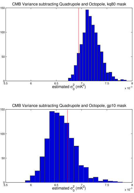
Let us study a possible relation between the low variance and the anomalous quadrupole-octopole alignment. In order to check the possible influence of these multipoles in our results, we remove the quadrupole and octopole from data and simulations, and repeat the analysis. The results plotted in Figure 8 and Figure 9 show that the data are now fully compatible with the simulations. The link between both anomalies is clear and they could have a common cause. Note that Figure 8 still reveals a slight dependence of the variance with the mask, i.e. the less pixels in the Galactic region are admitted, the lower is the variance of the data as compared to simulations. This could hint again to the presence of residual Galactic foreground contamination, but the variation is not statistically significant. Some authors, such as Slosar & Seljak (2004) or Abramo et al. (2009), pointed out foreground residuals as the cause of the quadrupole-octopole alignment. The results in this section show us that if there are Galactic foregrounds in the gp10 region, they mainly affect the quadrupole and octopole.
4.6 WMAP 7 year data
At the same time this paper was written, the WMAP team released a new version of the WMAP data (Jarosik et al., 2010). The data and masks given in the new release are very similar to the 5-year ones. We estimated the CMB variance for the 7-year data using the 7-year kq75 and kq85 masks obtaining and respectively, which differ less than and from the 5-year results listed in Table 2. Similar differences are found using the other masks. The lower instrumental noise of the 7-year data has a negligible effect in our variance estimation. The estimated variance for the 5-year data using the 7-year kq85 mask is which is a variation of with respect to the 7-year data result. Hence our results and conclusions remain unaffected by these small changes.
5 Conclusions
In this paper we compare the variance of the WMAP data to Gaussian simulations generated from the best fit angular power spectrum estimated from the data. Isotropy and Gaussianity are assumed to generate the simulations. Monteserín et al. (2008) already performed this comparison for the 3–year WMAP data, using the MKS variance estimator. They found that the variance of the data was lower than of the simulations.
Here we apply the UV estimator to the 5–year WMAP data. The UV estimator performs better than the MKS one due to a lower estimator variance and bias. We find again a low CMB variance with increased significance. The -value for the kq75 mask is . Performing the same analysis applying different exclusion masks we find a strong dependence of the variance with the used exclusion mask. The region near the Galactic plane shows a higher variance and compatibility with simulations, while the complementary region near the Galactic poles shows an anomalously low variance. We further localise the high-variance region, finding that the excess in variance is caused by about of the sky. This region, which we call the gp10 region, is located near the Galactic plane and shows an anomalously high variance (lower tail probability = ), whereas its complementary region (kq80 region) has an anomalously low variance (lower tail probability = ).
The relative difference of estimated variances between the WMAP gp10 and kq80 regions, is bigger than in of the simulations. Hence, this anisotropic distribution of the variance could be the cause of the observed anomaly. The angular power spectrum has been estimated applying the kq85 mask, admitting the high-variance region near the Galactic plane. Since isotropy is assumed, this high power is distributed over the whole sky when generating simulations. Comparing this high-variance simulations to the low variance region of the sky, they turn out to be incompatible.
Studying the relation of the low variance anomaly to the quadrupole-octopole alignment, we find that removing the quadrupole and octopole from data and simulations, the variance anomaly disappears. This link hints for a common cause of both anomalies.
There are several possible causes for both anomalies, namely unknown systematic effects, fortuitous alignment of quadrupole and octopole, Galactic foregrounds and cosmic defects. Any unknown systematic effect could be causing the anomaly, although there is no evidence for this hypothesis yet. A fortuitous alignment of quadrupole and octopole has been proven to be very unlikely (Bennett et al., 2010). A high variance in the region near the Galactic plane is a hint for Galactic foreground contamination. Furthermore we find strong evidence for foreground contamination in the Q band high-variance region. Slosar & Seljak (2004) already pointed out Galactic foregrounds as the cause of the alignment. Bennett et al. (2010) shows that masking some small regions in the sky the alignment disappears. In particular, masking some spots in the high-variance region, eliminates any significant alignment. This shows that the alignment is not robust and could be due to Galactic foregrounds in the high-variance region. Topological defects such as textures (Cruz et al., 2007b) could also be considered as an alternative explanation.
In our opinion the most likely hypothesis given the frequency dependence with respect to the Q band and the location of the high-variance region are Galactic foreground residuals. If this hypothesis was proven right, the cosmological parameter estimation could be affected in some extent. However, this has to be carefully analysed in future work.
Acknowledgments
We acknowledge financial support from the Spanish MCYT project AYA2007-68058-C03-02. PV acknowledges financial support from the Ramón y Cajal project. We acknowledge the use of the Legacy Archive for Microwave Background Data Analysis (LAMBDA). Support for LAMBDA is provided by the NASA Office of Space Science. This work has used the software package HEALPix (Hierarchical, Equal Area and iso-latitude pixelization of the sphere, http://www.eso.org/science/healpix), developed by K.M. Górski, E. F. Hivon, B. D. Wandelt, J. Banday, F. K. Hansen and M. Barthelmann; and the CAMB and CMBFAST software, developed by A. Lewis and A. Challinor and by U. Seljak and M. Zaldarriaga respectively.
References
- Abramo et al. (2009) Abramo L. R., Bernui A., Pereira T. S., 2009, JCAP, 12, 13
- Abramo et al. (2006) Abramo L. R., Sodré Jr. L., Wuensche C. A., 2006, Phys. Rev. D, 74, 083515
- Ayaita et al. (2009) Ayaita Y., Weber M., Wetterich C., 2009, ArXiv e-prints
- Bennett et al. (2003) Bennett C. L., et al., 2003, ApJS, 148, 1
- Bennett et al. (2010) Bennett C. L., et al., 2010, ArXiv e-prints
- Bernui (2009) Bernui A., 2009, Phys. Rev. D, 80, 123010
- Bernui et al. (2007) Bernui A., Mota B., Rebouças M. J., Tavakol R., 2007, A&A, 464, 479
- Bielewicz et al. (2005) Bielewicz P., Eriksen H. K., Banday A. J., Górski K. M., Lilje P. B., 2005, ApJ, 635, 750
- Bielewicz et al. (2004) Bielewicz P., Górski K. M., Banday A. J., 2004, MNRAS, 355, 1283
- Cayón (2010) Cayón L., 2010, MNRAS, 405, 1084
- Cayón et al. (2005) Cayón L., Jin J., Treaster A., 2005, MNRAS, 362, 826
- Cayon et al. (1991) Cayon L., Martinez-Gonzalez E., Sanz J. L., 1991, MNRAS, 253, 599
- Copi et al. (2006) Copi C. J., Huterer D., Schwarz D. J., Starkman G. D., 2006, MNRAS, 367, 79
- Copi et al. (2007) Copi C. J., Huterer D., Schwarz D. J., Starkman G. D., 2007, Phys. Rev. D, 75, 023507
- Copi et al. (2004) Copi C. J., Huterer D., Starkman G. D., 2004, Phys. Rev. D, 70, 043515
- Cruz et al. (2007a) Cruz M., Cayón L., Martínez-González E., Vielva P., Jin J., 2007a, ApJ, 655, 11
- Cruz et al. (2005) Cruz M., Martínez-González E., Vielva P., Cayón L., 2005, MNRAS, 356, 29
- Cruz et al. (2008) Cruz M., Martínez-González E., Vielva P., Diego J. M., Hobson M., Turok N., 2008, MNRAS, 390, 913
- Cruz et al. (2006) Cruz M., Tucci M., Martínez-González E., Vielva P., 2006, MNRAS, 369, 57
- Cruz et al. (2007b) Cruz M., Turok N., Vielva P., Martínez-González E., Hobson M., 2007b, Science, 318, 1612
- de Oliveira-Costa et al. (2004) de Oliveira-Costa A., Tegmark M., Zaldarriaga M., Hamilton A., 2004, Phys. Rev. D, 69, 063516
- Donoghue & Donoghue (2005) Donoghue E. P., Donoghue J. F., 2005, Phys. Rev. D, 71, 043002
- Eriksen et al. (2007) Eriksen H. K., Banday A. J., Górski K. M., Hansen F. K., Lilje P. B., 2007, ApJL, 660, L81
- Eriksen et al. (2005) Eriksen H. K., Banday A. J., Górski K. M., Lilje P. B., 2005, ApJ, 622, 58
- Eriksen et al. (2004) Eriksen H. K., Hansen F. K., Banday A. J., Górski K. M., Lilje P. B., 2004, ApJ, 605, 14
- Eriksen et al. (2004) Eriksen H. K., Novikov D. I., Lilje P. B., Banday A. J., Górski K. M., 2004, ApJ, 612, 64
- Frommert & Enßlin (2010) Frommert M., Enßlin T. A., 2010, MNRAS, 403, 1739
- Górski et al. (2005) Górski K. M., Hivon E., Banday A. J., Wandelt B. D., Hansen F. K., Reinecke M., Bartelmann M., 2005, ApJ, 622, 759
- Gruppuso & Burigana (2009) Gruppuso A., Burigana C., 2009, Journal of Cosmology and Astro-Particle Physics, 8, 4
- Gurzadyan et al. (2009) Gurzadyan V. G., Allahverdyan A. E., Ghahramanyan T., Kashin A. L., Khachatryan H. G., Kocharyan A. A., Kuloghlian H., Mirzoyan S., Poghosian E., Yegorian G., 2009, A&A, 497, 343
- Gurzadyan & Kocharyan (2008) Gurzadyan V. G., Kocharyan A. A., 2008, A&A, 492, L33
- Hansen et al. (2004) Hansen F. K., Banday A. J., Górski K. M., 2004, MNRAS, 354, 641
- Hansen et al. (2004) Hansen F. K., Cabella P., Marinucci D., Vittorio N., 2004, ApJL, 607, L67
- Hinshaw et al. (2009) Hinshaw G., et al., 2009, ApJS, 180, 225
- Hoftuft et al. (2009) Hoftuft J., Eriksen H. K., Banday A. J., Górski K. M., Hansen F. K., Lilje P. B., 2009, ApJ, 699, 985
- Jarosik et al. (2010) Jarosik N., et al., 2010, ArXiv e-prints
- Land & Magueijo (2005) Land K., Magueijo J., 2005, MNRAS, 357, 994
- Larson & Wandelt (2004) Larson D. L., Wandelt B. D., 2004, ApJL, 613, L85
- McEwen et al. (2005) McEwen J. D., Hobson M. P., Lasenby A. N., Mortlock D. J., 2005, MNRAS, 359, 1583
- Monteserín et al. (2008) Monteserín C., Barreiro R. B., Vielva P., Martínez-González E., Hobson M. P., Lasenby A. N., 2008, MNRAS, 387, 209
- Mukherjee & Wang (2004) Mukherjee P., Wang Y., 2004, ApJ, 613, 51
- Nolta et al. (2009) Nolta M. R., et al., 2009, ApJS, 180, 296
- Pietrobon et al. (2008) Pietrobon D., Amblard A., Balbi A., Cabella P., Cooray A., Marinucci D., 2008, Phys. Rev. D, 78, 103504
- Pietrobon et al. (2010) Pietrobon D., Cabella P., Balbi A., Crittenden R., de Gasperis G., Vittorio N., 2010, MNRAS, 402, L34
- Räth et al. (2007) Räth C., Schuecker P., Banday A. J., 2007, MNRAS, 380, 466
- Rossmanith et al. (2009) Rossmanith G., Räth C., Banday A. J., Morfill G., 2009, MNRAS, 399, 1921
- Schwarz et al. (2004) Schwarz D. J., Starkman G. D., Huterer D., Copi C. J., 2004, Physical Review Letters, 93, 221301
- Slosar & Seljak (2004) Slosar A., Seljak U., 2004, Phys. Rev. D, 70, 083002
- Vielva et al. (2004) Vielva P., Martínez-González E., Barreiro R. B., Sanz J. L., Cayón L., 2004, ApJ, 609, 22
- Vielva & Sanz (2010) Vielva P., Sanz J. L., 2010, MNRAS, pp 458–+
- Vielva et al. (2007) Vielva P., Wiaux Y., Martínez-González E., Vandergheynst P., 2007, MNRAS, 381, 932
- Wiaux et al. (2008) Wiaux Y., Vielva P., Barreiro R. B., Martínez-González E., Vandergheynst P., 2008, MNRAS, 385, 939
- Wiaux et al. (2006) Wiaux Y., Vielva P., Martínez-González E., Vandergheynst P., 2006, Physical Review Letters, 96, 151303