An Improved Calculation of the
Non-Gaussian Halo Mass Function
Guido D’Amicoa,b, Marcello Mussoc,
Jorge Noreñaa,b, Aseem Paranjapec
a SISSA, via Bonomea 265, 34136 Trieste, Italy
b INFN - Sezione di Trieste, via Bonomea 265, 34136 Trieste, Italy
c Abdus Salam International Centre for Theoretical
Physics
Strada Costiera 11, 34151, Trieste, Italy
Abstract
The abundance of collapsed objects in the universe, or halo mass
function, is an important theoretical tool in studying the effects of
primordially generated non-Gaussianities on the large scale
structure. The non-Gaussian mass function has been calculated by
several authors in different ways, typically by exploiting the
smallness of certain parameters which naturally appear in the
calculation, to set up a perturbative expansion. We improve upon the
existing results for the mass function by combining path integral
methods and saddle point techniques (which have been separately
applied in previous approaches). Additionally, we carefully account
for the various scale dependent combinations of small parameters which
appear. Some of these combinations in fact become of order unity for
large mass scales and at high redshifts, and must therefore be treated
non-perturbatively. Our approach allows us to do this, and also to
account for multi-scale density correlations which appear in the
calculation. We thus derive an accurate expression for the mass
function which is based on approximations that are valid
over a larger range of mass scales and
redshifts than those of other authors. By tracking the terms ignored
in the analysis, we estimate theoretical errors for our result and
also for the results of others. We also discuss the complications
introduced by the choice of smoothing filter function, which we take
to be a top-hat in real space, and which leads to the dominant errors
in our expression. Finally, we present a detailed comparison between
the various expressions for the mass functions, exploring the accuracy
and range of validity of each.
1 Introduction
The primordial curvature inhomogeneities, generated by the inflationary mechanism, obey nearly Gaussian statistics. The deviations from Gaussianity, while expected to be small, provide a unique window into the physics of inflation. For example, single-field slow-roll models of inflation lead to a small level of non-Gaussianity (NG), so that an observation of a large NG would indicate a deviation from this paradigm.
Until a few years ago, the main tool to constrain NG was considered to be the statistics of the cosmic microwave background (CMB) temperature field, since inhomogeneities at the CMB epoch are small and their physics can be described by a perturbative treatment. In recent years, however, thanks to observations and developments in the theory, the large-scale structure (LSS) of the universe has emerged as a complementary probe to constrain primordial NG. While it is true that the -point functions of the density field on small scales are dominated by the recent gravitational evolution, and do not reflect anymore the statistics of primordial perturbations, it turns out that the abundance of very massive objects, which form out of high peaks of the density perturbations, is a powerful probe of primordial NG. In this context, much attention has been given recently to three possible methods of constraining the magnitude and shape of the primordial NG with the LSS: the galaxy power spectrum, the galaxy bispectrum and the mass function. It was pointed out in Refs. [1, 2] that a NG of a local type induces a scale dependence on the galaxy power spectrum, thus making it a sensitive probe of the magnitude of local NG . From Ref. [3] one finds the following constraints: , already comparable with those obtained from CMB measurements in Ref. [4]: . The future is even more promising, with precisions of [5] and [6, 7, 8] being claimed for future surveys. The galaxy bispectrum is also a promising probe of NG as it could be more sensitive to other triangle configurations [9]. The mass function – which is the focus of this work, and which we discuss in detail below – has been used for example in Ref. [5] together with the scale dependent bias to produce forecasts for future surveys, and in Ref. [10] in an attempt to explain the presence of a very massive cluster at a large redshift as an indication of a large NG. For more references and information we refer the reader to reviews summarizing recent results on these topics [11, 12].
The formation of bound dark matter halos from initially small density perturbations, as seen in numerical simulations, is a complicated and violent process. Some insight into the physics involved has been gained from the study of analytical models. The quantity of interest is the halo mass function, defined as the number density of dark matter halos with a mass between and ,
| (1) |
where is the average density of the universe, is the variance of the density contrast filtered on some comoving scale corresponding to the mass , and the function is to be computed. Throughout this work, we will refer to itself as the mass function. A very useful tool in the analysis is the spherical collapse model [13], which predicts that the value of the linearly extrapolated density contrast of a spherical halo, at the time when the halo collapses, is , with a weak cosmology dependence. This value serves as a collapse threshold for determining which inhomogeneous regions will end up as collapsed objects. Using this idea, Press & Schechter [14] (PS) first computed the mass function in the case of Gaussian initial conditions. Their calculation however suffered from a problem of undercounting which affects the overall normalization – their approach does not count underdense regions embedded in larger overdense regions as eventually collapsed objects. To account for this discrepancy, PS introduced an ad-hoc factor of by demanding that the mass function be correctly normalized, such that all the mass in the universe must be contained in collapsed objects. In the excursion set approach, Bond et al. [15] resolved this issue and derived a correctly normalized mass function, for Gaussian initial conditions. They argued that the filtered density contrast follows a random walk as a function of the filtering scale, and the problem of computing is translated into the problem of finding the rate of “first crossing” of the barrier , whose solution is well-known. We will study this formalism in detail in section 3 for the more general non-Gaussian case.
Turning to non-Gaussianities, the most popular non-Gaussian mass functions are those due to Matarrese, Verde and Jimenez [16] (MVJ) and LoVerde et al. [17] (LMSV). Both groups used the PS approach, by modifying the probability density function for the (linearized) density contrast to describe non-Gaussian initial conditions. In their prescription, the relevant object is the ratio of non-Gaussian to Gaussian mass functions. The full mass function is usually taken as the product of and an appropriate Gaussian mass function as given by -body simulations, e.g. the Sheth & Tormen mass function [18]. It is not clear however that this is the correct way to proceed. Indeed, in a series of papers [19, 20, 21], Maggiore & Riotto (MR) presented a rigorous approach to the first-passage problem in terms of path integrals, and in Ref. [21] they pointed out that a PS-like prescription in fact misses some important non-Gaussian effects stemming from -point correlations between different scales (so-called “unequal time” correlators).
On the other hand, MR treated non-Gaussian contributions to by simply linearizing in the -point function of , i.e. by linearizing in the non-Gaussian parameter . Since the NG are assumed to be small, in the sense that the parameter satisfies , one might expect that such a perturbative treatment is valid. However, another crucial ingredient in the problem is that the length scales of interest are large, which leads to a second small parameter where . This is evident in the calculations of MR, who crucially use as a small parameter. Any perturbative treatment now depends not only on the smallness of and individually, but also on the specific combinations of these parameters which appear in the calculation. It is known (and we will explicitly see below) that a natural combination that appears is , which can become of order unity on scales of interest. The mass functions given by LMSV and MR therefore break down as valid series expansions when this occurs. Interestingly, MVJ’s PS-like treatment on the other hand involved a saddle point approximation, allowing them to non-perturbatively account for the term (which appears in an exponential in their approach). For a discussion, see Ref. [22].
It appears to us therefore, that there is considerable room for improvement in the theoretical calculation of the mass function. The goal of our paper is twofold. Firstly, we present a rigorous calculation of the mass function in the following way : (a) we use the techniques developed by MR in Refs. [19, 20, 21], which allow us to track the complex multi-scale correlations involved in the calculation, and (b) we demonstrate that MR’s approach can be combined with saddle point techniques (used by MVJ), to non-perturbatively handle terms which can become of order unity. This leads to an expression for the mass function which is valid on much larger scales than those presented by MR and LMSV. Secondly, by keeping track of the terms ignored, we calculate theoretical error bars on the expressions for resulting not only from our own calculations, but also for those of the other authors [16, 17, 21]. Since the terms ignored depend on in general, these error bars are clearly scale dependent. This allows us to estimate the validity of each of the expressions for the mass function at different scales, but importantly it also allows us to analytically compare between different expressions. In this paper we will not explicitly account for effects of the ellipsoidal collapse model [23, 24], since these are expected to be negligible on the very large scales which are of interest to us. For a recent treatment of ellipsoidal collapse effects in the presence of non-Gaussianities on scales where , see Lam & Sheth [25]. For a different approach to computing the non-Gaussian halo mass function, see Ref. [1], where the authors proposed that this mass function can be approximated as a convolution of the Gaussian mass function with a probability distribution function that maps between halos identified in Gaussian and non-Gaussian -body simulations. This probability distribution itself was approximated as a Gaussian, with mean and variance fit from simulations. While in practice this approach is easy to implement, it relies heavily on the output of -body simulations. Our approach, on the other hand, allows us to compute a mass function almost entirely from first principles.
This paper is organized as follows. In section 2 we fix some notation and briefly introduce the two most popular shapes of primordial NG, i.e. the local and equilateral ones. In section 3 we present our calculation of the mass function. In section 4 we discuss certain subtleties regarding the truncation of the perturbative series, and also compare with the other expressions for mentioned above. In section 5 we discuss the effects induced by some additional complications introduced in the problem due to the specific choice of the filter function [19], which we take to be a top-hat in real space, and due to the inclusion of stochasticity in the value of the collapse threshold (which is also expected to partially account for effects of ellipsoidal collapse) [20] . In section 6 we compare our final result Eqn. (43) with those of other authors, including theoretical errors for each, and conclude with a brief discussion of the results and directions for future work. Some technical asides have been relegated to the Appendices.
2 Models of non-Gaussianity
We need to relate the linearly evolved density field to the primordial curvature perturbation, which carries the information of the non-linearities produced during and after inflation. We start from the Bardeen potential on subhorizon scales, given by
| (2) |
where is the (comoving) curvature perturbation, which stays constant on superhorizon scales; is the transfer function of perturbations, normalized to unity as , which describes the suppression of power for modes that entered the horizon before the matter-radiation equality; and is the linear growth factor of density fluctuations, normalized such that in the matter dominated era. Then, the density contrast field is related to the potential by the Poisson equation, which in Fourier space reads
| (3) |
where we substituted Eqn. (2). Here, is the present time fractional density of matter (cold dark matter and baryons), and is the present time Hubble constant. The redshift dependence is trivially accounted for by the linear growth factor and in the following, for notational simplicity, we will often suppress it. All our calculations will use a reference CDM cosmology compatible with WMAP7 data [4], using parameters , , present baryon density , scalar spectral index and , where is the variance of the density field smoothed on a length scale of Mpc. For simplicity, for the transfer function we use the BBKS form, proposed in Bardeen et al. [23]:
| (4) |
where with a shape parameter that accounts for baryonic effects as described in Ref. [26]. For more accurate results, one could use a numerical transfer function, as obtained by codes like CMBFAST [27] or CAMB [28]; the results are not expected to be qualitatively different.
In order to study halos, which form where an extended region of space has an average overdensity which is above threshold, it is useful to introduce a filter function , and consider the smoothed density field (around one point, which we take as the origin),
| (5) |
where is the Fourier transform of the filter function. For all numerical calculations we will use the spherical top-hat filter in real space, whose Fourier transform is given by
| (6) |
This choice allows us to have a well-defined relation between length scales and masses, namely with . However it introduces some complexities in the analysis, which we will comment on later. By using Eqns. (5) and (3) we have, for the -point function,
| (7) |
where the subscript denotes the connected part, and analogous formulae are valid for the higher order correlations.
2.1 Shapes of non-Gaussianity
The function encodes information about the physics of the inflationary epoch. By translational invariance, it is proportional to a momentum-conserving delta function:
| (8) |
where the (reduced) bispectrum depends only on the magnitude of the ’s by rotational invariance. According to the particular model of inflation, the bispectrum will be peaked about a particular shape of the triangle. The two most common cases are the squeezed (or local) NG, peaked on squeezed triangles , and the equilateral NG, peaked on equilateral triangles . Indeed, one can define a scalar product of bispectra, which describes how sensitive one is to a NG of a given type if the analysis is performed using some template form for the bispectrum. As expected, the local and equilateral shapes are approximately orthogonal with respect to this scalar product [29]. We will now describe these two models in more detail.
The local model: The local bispectrum is produced when the NG is generated outside the horizon, for instance in the curvaton model [30, 31] or in the inhomogeneous reheating scenario [32]. In these models, the curvature perturbation can be written in the following form,
| (9) |
where is the linear, Gaussian field. We have included also a cubic term, which will generate the trispectrum at leading order. The bispectrum is given by
| (10) |
where “cycl.” denotes the 2 cyclic permutations of the wavenumbers, and is the power spectrum given by . The trispectrum is given by
| (11) |
The equilateral model: Models with derivative interactions of the inflaton field [33, 34, 35] give a bispectrum which is peaked around equilateral configurations, whose specific functional form is model dependent. Moreover, the form of the bispectrum is usually not convenient to use in numerical analyses. This is why, when dealing with equilateral NG, it is convenient to use the following parametrization, given in Ref. [36],
| (12) |
This is peaked on equilateral configurations, and its scalar product with the bispectra produced by the realistic models cited above is very close to one. Therefore, being a sum of factorizable functions, it is the standard template used in data analyses.
3 Random walks and the halo mass function
We now turn to the main calculation of the paper. The non-Gaussian halo mass function can be obtained by calculating the barrier first crossing rate of a random walk with non-Gaussian noise, in the presence of an absorbing barrier. This can be done perturbatively, starting from a path integral approach as prescribed by MR [19, 21] and the mass function can be shown to be . As discussed by MR, the calculation of involves certain assumptions regarding the type of filter used and also the location of the barrier. In particular, the formalism is simplest for a sharp filter in -space, and using the spherical top-hat of Eqn. (6) introduces complications in the form of non-Markovian effects. Further, in order to make the spherical collapse ansatz more realistic and obtain better agreement with -body simulations, MR show that it is useful to treat the location of the barrier as a stochastic variable itself, and allow it to diffuse. For the time being, we will ignore these complications, and will return to their effects in section 5.
To make the paper self-contained, we begin with a brief review of the path integral approach to the calculation of the mass function. The reader is referred to Ref. [19] for a more pedagogical introduction. In the path integral approach, one treats the variance as a “time” parameter, , and considers the random walk followed by the smoothed density field as this “time” is increased in discrete steps starting from small values (equivalently, as is decreased from very large values). Here is a stochastic quantity in real space due to the stochasticity inherent in the initial conditions. We use the notation to distinguish the stochastic variable from the values it takes, which will be noted by below. We probe this stochasticity by changing the smoothing scale at a fixed location , thus making the variable perform a random walk, which obeys a Langevin equation
| (13) |
with a stochastic noise whose statistical properties depend on the choice of filter used. In particular, for a top hat filter in -space, the noise is white, i.e. its -point function is a Dirac delta [15],
| (14) |
The random walk can be described as a trajectory which starts with taking the value at (or which is the homogeneous limit), then taking values at times , finally arriving at at time , with a discrete timestep . The probability that the trajectory crosses the barrier at at a time larger than some (i.e. at scales smaller than the corresponding or ), is the same as the probability that the trajectory did not cross the barrier at any time smaller than , so that
| (15) |
where the probability density over the space of trajectories, is defined as
| (16) |
where is the Dirac delta distribution. The first crossing rate is given by the negative time derivative of , , and the mass function is then . In Eqn. (16) one can write the Dirac deltas using the integral representation , to obtain
| (17) |
The object is the exponential of the generating functional of the connected Green’s functions, and can be shown to reduce to [37]
| (18) |
where is the connected -point function of , with the short-hand notation .
3.1 Halo mass function: Gaussian case, sharp- filter
In the Gaussian case, all connected -point correlators vanish except for , and in the Markovian (sharp- filter) case which we are considering, the -point function becomes , where is the minimum of and . The resulting -dimensional Gaussian integral can be handled in a straightforward way to obtain
| (19) |
where we follow MR’s notation and use the superscript “gm” to denote “Gaussian Markovian”. As MR have shown [19], the resulting expression for in the continuum limit is simply
| (20) |
where we use the notation . (This in principle also includes the redshift dependence of the collapse threshold , see below.) This expression for the continuum limit probability is of course a well-known result going back to Chandrasekhar [38]. This leads to the standard excursion set result for the Gaussian mass function ,
| (21) |
where we use the subscript PS (for Press-Schechter), to conform with the conventional notation for this object.
3.2 Halo mass function: non-Gaussian case, sharp- filter
In the non-Gaussian case (but still retaining the sharp- filter), the probability density also gets contributions from connected -point correlators with , since these in general do not vanish. These can be handled by using the relation , with . A straightforward calculation then shows the mass function to be
| (22) |
where it is understood that one takes the continuum limit before computing the overall derivative with respect to . We will find it useful to change variables from (, ) to (, ), in which case the partial derivative becomes
| (23) |
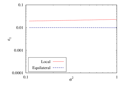
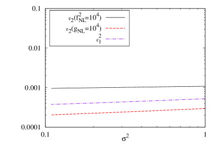
It is also useful at this stage to take a small detour and introduce some notation which we will use throughout the rest of the paper. We define the scale dependent “equal time” functions
| (24) |
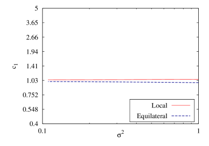
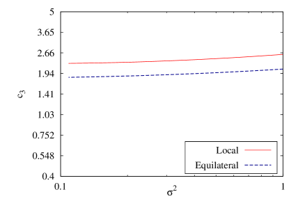
which as we will see, remain approximately constant over the scales of interest. We assume the ordering with , which can be motivated from their origin in inflationary physics, where one finds , , etc111Notationally we distinguish the order parameter from the specific NG functions and .. Typically we expect for . Fig. 1 shows the behaviour of and in the local and equilateral models, as a function of . We see e.g. that in the local model is comparable to . In the literature one usually encounters the reduced cumulants , which are related to the by , and so on. The motivation for using the comes from the study of NG induced by nonlinear gravitational effects. However, as we see from Fig. 1, when studying primordial NG it is more meaningful to consider the which are approximately scale-independent and perturbatively ordered.
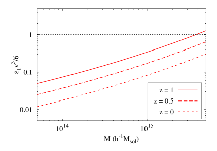
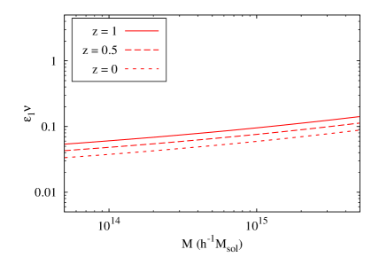
We will soon see that a natural expansion parameter that arises in the calculation has the form , and we therefore require that the mass scales under scrutiny are not large enough to spoil the relation . It turns out that observationally interesting mass scales can nevertheless be large enough to satisfy . Fig. 2 shows the behaviour of and at different redshifts, as a function of mass, in our reference CDM model for local type NG, with . The behaviour for the equilateral NG is qualitatively similar.
The redshift dependence of these quantities comes from the definition of ,
| (25) |
where we denote the usual spherical collapse threshold as , reserving for the full, redshift dependent quantity, and is a parameter accounting for deviations from the simplest collapse model. In the standard spherical collapse picture we have . A value of different from unity (specifically ) can be motivated by allowing the collapse threshold to vary stochastically [20], as we will discuss in section 5. We will soon see that the object appears naturally in the calculation, and to be definite we will assume for now. In section 4 we will discuss the effects of relaxing this condition and probing smaller length scales.
We now turn to the “unequal time” correlators appearing in Eqn. (22). Since we are concerned with large scales, we are in the small limit, and following MR we expand the -point correlators around the “final time” . We can define the Taylor coefficients
| (26) |
and then expand
| (27) |
For the -point function we will have an analogous expression involving coefficients .
Since calculations involving a general set of coefficients , , etc. are algebraically rather involved, we find it useful to first consider an example in which these coefficients take simple forms. In this toy model we assume that the are exactly constant, and moreover that the -point correlators take the form222Throughout the paper we will consider at most -point correlators. This truncation is justified given our assumptions, as we will see later.
| (28) |
For clarity, we will display details of the calculation only for this model. We have relegated most of the technical details of our calculation to Appendix A. In Appendix A.1 we show that the mass function for this model can be brought to the form
| (29) |
where we ignore terms like . The remaining exponentiated derivative can be handled using a saddle point approximation. We show how to do this in Appendix A.2. The expression for the mass function works out to
| (30) |
which superficially at least, is comprised of two series expansions, one in the exponential and one as a polynomial, both based on the small parameter (see however the next section).
This derivation assumed that and are constant, and that the unequal time correlations are given by Eqn. (28). It is straightforward to relax these assumptions and perform the calculation with the exact structure of the correlations. Appendix A.3 shows how to do this, and the result is
| (31) |
where the functions are defined in Eqn. (A.17) and characterize the behaviour of the unequal time correlations. In our toy model above, the reduce to unity. Indeed, as a check we see that the expression in (31) reduces to Eqn. (30) if we take , to be constant and set the to unity.
One issue which we have ignored so far, is that the definition of involves the variance of the non-Gaussian field. Computationally it is more convenient to work with the variance of the Gaussian field in terms of which cosmological NG are typically defined. We should then ask whether this difference will require changes in our expressions for . We start by noting that this difference in variances is of order . For example, in the local model one has where is an overall normalization constant, and are scale dependent functions of comparable magnitude on all relevant scales, and is estimated as . We therefore have . However, with our assumption that , we see that this correction is actually of order , which we have been consistently ignoring. We will see that even when we relax the assumption and probe smaller scales where , this correction can still be consistently ignored. Hence we can safely set in all of our expressions.
4 Consistency of the truncation
4.1 Comparative sizes of terms in the mass function
Now that all the derivative operators which we consider important have been accounted for, we can check whether our final result is consistently truncated, i.e. whether we have retained all terms at any given order in the expansion. Symbolically, our current result for the mass function can be written as
| (32) |
with the understanding that coefficients are computed (but not displayed) for all terms except those indicated by the symbols. Also, refers to both and .
Since the expansions involve two parameters, and , they make sense only if we additionally prescribe a relation between these parameters. So far we assumed that is fixed and is such that , which was based on the observation that the term naturally appears in the exponent and is not restricted in principle to small values. In Appendix B.1 we discuss this condition in more detail, and also analyse the consequences of relaxing this condition and probing smaller mass scales. We find that for observationally accessible mass scales larger than the scale where , the single expression
| (33) |
is parametrically consistent as it stands – the terms ignored are smaller than the smallest terms retained – and in fact it remains a very good approximation even when , since the only “inconsistent” term then is , whose effect reduces as increases. On scales where and lower, the theoretical error becomes comparable to or larger than the quadratic term in the exponential. Plugging back all the coefficients, we have the following result for the mass function (excluding filter effects, see section 5),
| (34) |
4.2 Comparing with previous work
In this subsection we compare our results with previous work on the non-Gaussian mass function. As mentioned in the introduction, this quantity has been computed by several authors in different ways [16, 17, 21]. If one considers the range of validity of the perturbative expansion, the strongest result so far has been due to MVJ [16], who explicitly retain the exponential dependence on . Their expression for can be written as333The analysis presented by MVJ in fact allows one to retain terms like in the exponential as well, and we have seen that when , these terms are as important as the polynomial term retained by MVJ. However, since the MVJ expression misses unequal time effects of order anyway, it is reasonable to compare our results with the expression (35), which is also the one used by most other authors (see e.g. Refs. [39, 40]).
| (35) |
The major shortcoming of their result is that it is based on a Press-Schechter like prescription, and must therefore be normalized by an appropriate Gaussian mass function, typically taken to be the one due to Sheth & Tormen [18]. Additionally, it always misses the contributions due to the unequal time correlators, which contribute to the terms , , etc. in Eqn. (34). When one considers formal correctness on the other hand, MR have presented a result based on explicit path integrals, which accounts for the unequal time contributions, and which also does not need any ad hoc normalizations (in this context see also Lam & Sheth [25]). Indeed, our calculations in section 3 were based on techniques discussed by MR in Refs. [19, 21]. As we discuss below however, the fact that MR do not explicitly retain the exponential dependence of , means that their result is subject to significant constraints on the range of its validity. Their expression for , ignoring filter effects, is444We have corrected a typo in MR’s result [21] : the object they define as should appear with an overall positive coefficient in their Eqns. (85), (87) and (92).
| (36) |
This expression is precisely what one obtains by linearizing our expression (34) in , which serves as a check on our calculations. LMSV [17] present a result based on an Edgeworth expansion of the type encountered when studying NG generated by nonlinear gravitational effects [41]. The result most often quoted in the literature is their expression linear in (and hence in ), which is
| (37) |
In Appendix B.3 of Ref. [17], LMSV also give an expression involving and , which can be written as
| (38) |
where the are the Hermite polynomials of order . This expression was used by LMSV only as a check on the validity of their linear expression. By comparing with our expression which is non-perturbative in , we will see below that these quadratic terms in fact significantly improve LMSV’s prediction.
Sticking to the linearized results, we see that the expressions of both MR and LMSV have the symbolic form
| (39) |
where the ellipsis denotes all terms of the type , , etc., as well as all terms containing . As we have seen, deciding where to truncate the expression for is not trivial, and using our more detailed expression we can ask whether the expression (39) is consistent at all the relevant length scales. Immediately, we see that this expression cannot be correct once becomes close to unity. In Appendix B.2 we discuss the situation for MR and LMSV at smaller mass scales.
5 Effects of the diffusing barrier and the filter
In Ref. [20], MR showed that the agreement between a Gaussian mass function calculated using the statistics of random walks, and mass functions observed in numerical simulations with Gaussian initial conditions, can be dramatically improved by allowing the barrier itself to perform a random walk. This approach is motivated by the fact that the ignorance of the details of the collapse introduces a scatter in the value of the collapse threshold for different virialized objects. The width of this scatter was found by Robertson et al. [42] to be a growing function of , which is consistent with the physical expectation that deviations from spherical collapse become relevant at small scales. The barrier can thus be treated (at least on a first approximation) as a stochastic variable whose probability density function obeys a Fokker-Planck equation with a diffusion coefficient , which can be estimated numerically in a given -body simulation. In particular, MR found using the simulations of Ref. [42].
Conceptually, the variation of the value of the barrier is due to two types of effects, one intrinsically physical and one more inherent to the way in which one interprets the results of simulations. From a physical point of view, the dispersion accounts for deviations from the simple model of spherical collapse, for instance the effects of ellipsoidal collapse, baryonic physics, etc. On the other hand, the details of the distribution of the barrier (and therefore the precise value of ) will depend on the halo finder algorithm used to identify halos in a particular simulation, since different halo finders identify collapsed objects with different properties. MR concluded that the final effect of this barrier diffusion on large scales can be accounted for in a simple way, by changing where . In practice this change is identical to the one proposed by Sheth et al. [24]555A potential issue in this argument lies in the assumption of a linear Langevin equation for the stochastic barrier , resulting in a simple Fokker-Planck equation with a constant like the one in MR, while the distribution of was found to be approximately log-normal (and therefore non-Gaussian) in Ref. [42]. One can see that a Langevin equation of the type (which would produce a log-normal distribution) can be approximated by , whenever the fluctuations around are small, and gives a constant diffusion coefficient as long as is constant. Although both approximations are reasonable on the scales of interest, non-Gaussian and scale dependent corrections to the barrier diffusion should be studied, since in principle they could be of the same order as the other corrections retained here. This investigation is left for future work.. As MR argue in section 3.4 of Ref. [21], this barrier diffusion effect can also be accounted for in the non-Gaussian case, again by the simple replacement of . It is easy to see that their arguments go through for all our calculations as well, and we have implemented this change in our definition of in Eqn. (25), setting .
In Ref. [19], MR also accounted for the non-Markovian effects of the real space top-hat filter, as opposed to the sharp- filter for which the results of section (3) apply. This is done by writing the -point function calculated using the real space top-hat filter, as the Markovian value plus a correction, , and noting that the correction remains small over the interesting range of length scales. In fact, MR show that a very good analytical approximation for the symmetric object , is
| (40) |
where in our case we find , with measured in Mpc. The mass function is then obtained by perturbatively expanding in , with the leading effect being due to the integral
which on evaluation leads to
| (41) |
where the subscript stands for Gaussian noise with the top-hat filter in real space, and introduces a weak explicit dependence. In Ref. [21] MR proposed an extension of this result to the non-Gaussian case, by assuming that all the non-Gaussian terms that they computed with the sharp- filter, would simply get rescaled by the factor at the lowest order, but otherwise retain their coefficients. Symbolically, their result (Eqn. 88 of Ref. [21]) is
| (42) |
with the specific coefficients of the , and terms being identical to those in Eqn. (36). However, the coefficient of e.g. the term arises from the action of an operator combining with the first unequal time operator , and there is no simple way of predicting its exact value beforehand. Since MR explicitly neglect such “mixed” terms, their formula is not strictly inconsistent, as long as one keeps in mind that the theoretical error in their expression is of the same order as the terms that they include. However, if one wants to consistently retain such terms, a detailed calculation is needed666Notice that this issue is completely decoupled from the subtleties in truncation discussed in section 4 – this problem remains even at scales where MR’s expression is formally consistent.. Our calculations (not displayed) indicate that the coefficient of the term depends on certain details of the continuum limit of the path integral near the barrier, which require a more careful study. We are currently investigating methods of computing these effects. At present however, we conclude that the mixed terms involving both filter effects and NG, must be truncated at order .
Finally, the filter-corrected mass function is also subject to effects of barrier diffusion. Here we make the same assumptions as MR do in Ref. [20], namely that the barrier location satisfies a Langevin equation with white noise and diffusion constant , which can be accounted for by replacing . However, it is difficult to theoretically predict the unequal time behaviour of the barrier correlations, and these simple assumptions must also be tested, perhaps by suitably comparing with the detailed results of Robertson et al. [42]. We leave this for future work. Our final expression for the mass function, corrected for effects of the diffusing barrier and the top-hat real space filter, is
| (43) |
where we have chosen to account for the scale independent error arising from filter effects, as an overall normalization uncertainty, and have explicitly displayed the orders of the various terms we ignore. Here is given by Eqn. (21) with defined in Eqn. (25).
To summarize, Eqn. (43) gives an analytical expression for the non-Gaussian mass function. This expression is based on approximations that are valid over a larger range of length scales than the ones presented by MR and LMSV, and incorporates effects which are ignored in the expression presented by MVJ and LMSV. Like all these other mass functions, it suffers from the errors introduced by filter effects. However, the largest of these can be accounted for as an overall normalization constant, which can be fixed using, for instance, results of a Gaussian simulation. Among the NG functions , and the which appear in the mass function, the most important ones over the mass range of interest are , and which are nearly constant. In principle though, all these functions must be computed numerically for every mass scale of interest, and indeed all the plots in this paper use the results of such numerical calculations. However, since this is somewhat tedious to do in practice, in Table 1 we provide analytical approximations for , , , and , for the local and equilateral case as a function of . As mentioned earlier, all these quantities are independent of redshift, although they depend on the choice of cosmological parameters in a complicated way in general due to the presence of the transfer function in their definitions. However, the dependence on is simple, and one can check that we have , and that the are independent of . Recall that the are also independent of and . For completeness, in Table 1 we also give approximations for the filter parameters and which appear in the mass function, as functions of .
| Parameter | Fitting form | ||
|---|---|---|---|
| Local NG | |||
| Parameter | Fitting form | ||
| Equilateral NG | |||
| Filter | |||
6 Results and Discussion
In this section we conclude with our final results for the non-Gaussian halo mass function, comparing our approach with previous work. In principle, we should compare the full expressions for the mass functions of various authors with ours. However, recall that for MVJ and LMSV one has to multiply an analytically predicted ratio with a suitable Gaussian mass function based on fits to simulations. It is not clear how to compute theoretical error bars on the latter. On the other hand, the object itself is an unambiguous theoretical prediction of every approach, that is MVJ, LMSV, MR and our work, and we can compute theoretical errors on it. In this work, we will restrict ourselves to comparing the different expressions for . In future work, we hope to compare both and the full mass function with the results of -body simulations.
In Fig. 3 and Fig. 4 we plot the ratio , respectively without and with the filter effects, at redshift . In this way we can explicitly disentangle the errors due to an approximate treatment of non-Gaussian effects, from those due to the filter effects. We compare our expression (43) with the expressions of MR (36), LMSV (37) and (38), and of MVJ (35). Notice that, when considering the filter effects, the Gaussian function that enters in the ratio is defined to be the function with (i.e. without NG but with filter effects when present). We use the local model, setting and , and use the reference CDM cosmology described in section 2. We do not explicitly show the final results for the equilateral model, but they are qualitatively similar. As is commonly done in the literature, we modify the LMSV and MVJ curves by applying the Sheth et al. correction of . An identical correction is already present in the expressions (43) and (36) due to the barrier diffusion. We set , which is the value inferred by MR in Ref. [20] using the simulations of Robertson et al. [42]. We wish to emphasize a feature that our calculation shares with that of MR, which is that the constant is the only parameter whose value depends on the output of -body simulations. The rest of the calculation for the mass function is completely analytical and from first principles.
To make the comparison meaningful, we introduce theoretical error bars on the curves. These error bars have no intrinsic statistical meaning – they simply keep track of the absolute magnitude of the terms that are ignored in any given prescription for computing the mass function. As we have discussed at length in section 4, these theoretical errors are scale dependent. The estimated error magnitude for each point is the maximum among the terms ignored in the expression. More explicitly, the errors for the linearized LMSV expression (37) are estimated as the maximum of which comes from the expansion of the exponential, which is the order of the largest unequal time terms missing, and which comes from the filter effects. The errors for the LMSV expression (38) are similarly estimated as the maximum of , and . The largest error for the MVJ expression (35) is the maximum of (unequal time terms) and (filter effects). Finally, the error for the MR expression (36) is the maximum of from the expansion of the exponential, from the largest unequal time terms ignored, and and from the filter effects. We include the filter effects and the associated errors only in Fig. 4.
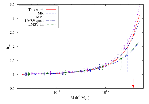
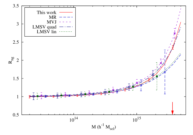
From these figures, we can draw some interesting conclusions. First of all, we see that it is important to retain terms which are quadratic in the NG, either with a saddle point method like in MVJ and in our formula, or by expanding the exponential up to second order, like in LMSV. Actually, we argue that it is correct to keep the exponential, otherwise the expansion breaks down when is of order unity. We notice in passing that the term proportional to which comes from the trispectrum, partially cancels with the term. Secondly, comparing our expression with MVJ’s, we can observe that keeping the unequal time terms allows us to sensibly reduce the theoretical errors due to the approximate treatment of NG. In fact, if these terms are missing, they provide the largest theoretical error on large scales. Instead, the largest theoretical error on small scales comes from the approximations involved in dealing with a real space top-hat filter, as is apparent from Fig. 4.
To conclude, in this work we have calculated the non-Gaussian halo mass function in the excursion set framework, improving over previous calculations. We started from a path integral formulation of the random walk of the smoothed density field, following Ref. [19]. This allows us to take into account effects due to multi-scale correlations of the smoothed density field (“unequal time” correlations), and due to the real space top-hat filter, which generates non-Markovianities in the random walk. We recognize two small parameters in which we perturb: , defined below Eqn. (24), which measures the magnitude of the primordial NG; and , which is small on very large scales. In order to do a consistent expansion and to estimate the theoretical errors, one must study the (scale dependent) relation between these two parameters, which we have discussed in Sec. 4. We then used saddle point techniques which allowed us to non-perturbatively retain the dependence on , which naturally appears in the calculation and whose magnitude becomes of order unity at high masses and high redshift. Finally, we included effects due to the choice of filter function and due to deviations from spherical collapse, as explained in Sec. 5. Our final result is presented in Eqn. (43), which we reproduce here:
| (44) |
In Table 1 we provide analytical approximations for the various parameters that appear in this expression, which in general must be computed numerically. We also considered other expressions for the mass function found in the literature, which use different expansion methods but do not estimate the theoretical errors. We estimated the theoretical errors for each formula, and we show comparative plots in Fig. 3 and Fig. 4. In our work we have improved over the calculations of MVJ [16] and LMSV [17] (who ignore unequal time correlations) and of MR [21] (who do not retain the exponential dependence on ). We have also demonstrated that the (linearized) result of LMSV can be significantly improved by retaining the quadratic terms of their calculation which are usually ignored in the literature. We find that at large scales and high redshifts, the biggest theoretical errors are introduced by ignoring the exponential dependence on , followed by the neglect of unequal time correlations. The errors on our expression (44) are therefore significantly smaller than those of the others. The strength of our approach lies in the combination of path integral methods as laid out by MR [21], and the saddle point approximation as used by MVJ [16].
Our work can be continued in several directions. First, a thorough calculation of the effects due to the choice of the filter should be performed, since they lead to significant uncertainties in our final expression. This would include a study of the details of the continuum limit of the path integral near the barrier, and also a study of the statistics of the barrier diffusion process in the presence of filter effects. Second, a comparison with -body simulations should be performed, in order to quantitatively assess the possibility of constraining NG using our work. Third, it would be interesting to study how to account for the effects of ellipsoidal collapse, in a framewrok such as the one employed in this paper. Finally, an application to the void statistics along the same lines should be feasible. The problem here is made more interesting by the presence of two barriers, as discussed by Sheth & van de Weygaert [43], and since voids probe larger length/mass scales than halos, they constitute a promising future probe of primordial NG [44].
Acknowledgements
It is a pleasure to thank Stefano Borgani, Paolo Creminelli, Francesco Pace, Emiliano Sefusatti, Ravi Sheth, Licia Verde and Filippo Vernizzi for useful discussions.
Appendix
Appendix A Mass function calculation
A.1 Equal time vs. unequal time terms
In this appendix we show how the exponentiated derivative operator in the path integral can be handled by separating the contributions of the equal time and unequal time correlations. While this calculation assumes the toy model introduced in Eqn. (28), it easily generalizes to the more realistic case as we discuss later.
Using the first few terms of the unequal time expansions, in our toy model one can write
| (A.1) | |||
| (A.2) |
These derivative operators are exponentiated in the path integral, and act on . One simplification that occurs in our toy model, is that the path integral in Eqn. (22) becomes a function only of (although this is not obvious at this stage), and hence eventually only the part of the overall derivative contributes. However, the structure of the exponentiated derivatives is still rather formidable. Moreover, the truncation of the series at this stage is based more on the intuition that higher order terms should somehow be smaller, rather than on a strict identification of the small parameters. In fact, we will see in detail in section 4 that the issue of truncation involves several subtleties.
To make progress, it helps to analyze the effect on of each of the terms in the above series, before exponentiation. The leading term in Eqn. (22) involves the multiple integral of , which is just the quantity encountered in Eqn. (20). The operator acts on the error function to give the Gaussian rate of Eqn. (21). Next, notice that the action of the operator on any function under the multiple integral, is simply
| (A.3) |
Using this, and the fact that , we see that the leading term in Eqn. (A.1) (i.e. the term with no powers of ), leads to a term involving
The problem with this term is that the quantity can be of order unity, and hence cannot be treated perturbatively. To be consistent, we should keep all terms involving powers of . Luckily, this can be done in a straightforward way due to the result in Eqn. (A.3). We see that the entire exponential operator in Eqn. (22) can be pulled across the multiple integral and converted to acting on the remaining integral. Similarly, the operator can be pulled out and converted to , and the same applies for all such equal time operators. We will see later that the action of these operators can be easily accounted for, using a saddle-point approximation. To summarize, the function at this stage is given by
| (A.4) |
Now consider the action of the individual terms in the remaining exponential under the integrals, but without exponentiation. From MR [21], we have the following results777The terms in Eqns. (A.5a), (A.5b) and (A.5c) are, upto prefactors, the integrals of what MR denote as , and respectively in Ref. [21].,
| (A.5a) | ||||
| (A.5b) | ||||
| (A.5c) | ||||
where we have defined
| (A.6) |
where is an incomplete gamma function. Let us focus on the term in Eqn. (A.5a). If we linearize in in Eqn. (A.4), then this term appears with acting on it, leading to . This term can therefore be treated perturbatively. Similarly, one can check that the terms given by Eqns. (A.5b) and (A.5c) also lead to perturbatively small quantities, which are in fact further suppressed compared to by powers of . Specifically, one obtains terms involving which, for large , reduces to .
A few comments are in order at this stage. First, this ordering in powers of is a generic feature of integrals involving an increasing number of powers of being summed. This can be understood in a simple way from the asymptotic properties of the incomplete gamma function, as we show in Appendix C. We are therefore justified in truncating the Taylor expansion of the unequal time correlators, even though superficially (on dimensional grounds) each term in the series appears to be equally important. Secondly, we have not yet accounted for the effect of the exponential derivatives. In fact we will see in the next section that when , it is these terms that impose stricter conditions on the series truncations. For now, however, we have no guidance other than the fact that if we account for one term of order , then we should account for all terms at this order. Given this, note that for we have , and hence the terms arising from Eqns. (A.5b) and (A.5c) are of order . To consistently retain them, we must therefore also retain the term linear in and the one quadratic in , when expanding the exponential. These involve the following quantities:
| (A.7a) | ||||
| (A.7b) | ||||
where we have used the result (A.3), and in Eqn. (A.7b) also the identity
| (A.8) |
We now see that the result of the path integral depends only on . Putting things together and computing the overall derivative, we find the result in Eqn. (29).
A.2 Saddle point calculation
To compute the action of the exponentiated derivative operators, we start by writing the expression in square brackets in Eqn. (29) in terms of its Fourier transform, using the relations888We are using a regulator which shifts the pole at in the last expression in Eqn. (A.9), to where is real, positive and small.
| (A.9) |
Together with the identity , for constant and , this gives
| (A.10) |
where is the truncated series given by
| (A.11) |
The integral in eq. (A.10) can be performed using the saddle point approximation. We write it as
| (A.12) |
where
| (A.13) |
The location of the saddle point, , is the solution of , and the saddle point approximation then tells us that
| (A.14) |
(see Appendix D for a discussion of the errors introduced by this approximation). It turns out that in order to obtain correctly up to order , we only need correct up to order . The expression for at the relevant order is,
| (A.15) |
and solving for perturbatively up to order , we find
| (A.16) |
This leads to the expression for in Eqn. (30).
A.3 Result with full unequal time terms
In the more realistic case of slowly-varying , we choose to parametrize the coefficients and (see Eqn. (26)) in a convenient way as follows :
| (A.17) |
where the coefficients are smoothly varying functions and depend on the NG model. They are defined in such a way that they all reduce to unity in the toy model defined by Eqn. (28). Fig. 5 shows the behaviour of , and with , for the local and equilateral models. The and are independent of redshift by construction, since the linear growth rate always drops out in their definitions. Further, the do not depend on the values of and . One can then use the definitions of and the to prove the following useful relations
| (A.18) |
The calculation of the mass function for this general case proceeds completely analogously to that for the toy model, apart from a few subtleties which we will discuss later.

In this case Eqn. (A.4) is replaced with
| (A.19) |
wher the function can be shown to be
| (A.20) |
The expression in Eqn. (A.19) can be evaluated analogously to Eqn. (29), since the additional derivatives pose no conceptual difficulty. The result of the saddle point calculation, correct up to quadratic order assuming , and after using the relations (A.18), is given in Eqn. (31).
Appendix B Truncation of the perturbative series
B.1 Analysis of “transition points”
In this appendix we analyse the consistency of our series truncation at various mass scales. When , in the polynomial in (32) we retain the terms , , and we discard . It would seem that our expression is then correct upto order . However, the terms discarded in the exponential have the form . The error we are making is thus of the same order as the smallest terms we are retaining, and it therefore makes sense to also ignore all the terms of order which we computed in the polynomial. The consistent expression when is then given by
| (B.1) |
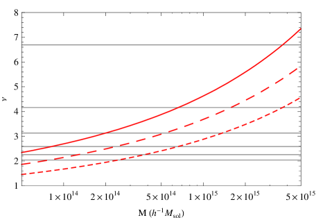
Clearly, similar arguments can be applied at smaller scales where, e.g. one might have , etc. It is then important to ask which mass scales correspond to these “transition points”. In Fig. 6 we plot given by Eqn. (25) in an observationally interesting mass range, for three different redshifts. The horizontal lines mark the transition points where becomes equal to (from top to bottom) , , , , and . We fix which follows from the fact that in the local model with we have (see Fig. 1), and the expression for contains the quantity in the exponential. From the intersections of the horizontal lines with the curves, we see that different transition points are relevant at different redshifts, and their locations also obviously depend on the value of . For example, we find that the transition point where , remains accessible even when is an order of magnitude smaller (with , this transition occurs at ). The transitions at on the other hand, are not accessible for this level of NG. The transition at is therefore observationally very interesting.
We will now discuss in some detail the truncation of our expression for , at various transition points. The goal is to try and settle on a single expression which is valid over a wide range of scales (i.e. across several transition points). This can then be applied without worrying about truncation inconsistencies. Of course, the order of the discarded terms will then depend on the particular transition point being considered, leading to a scale dependent theoretical error.
B.1.1
At this transition point, the terms we retain in the exponential are
while discarding . In the polynomial meanwhile, we retain
while discarding
Our expression (32) therefore retains all terms correctly up to order , and is consistent. With some foresight however, it turns out to be more convenient to degrade this expression somewhat by also discarding the polynomial quadratic term . The remaining expression,
| (B.2) |
is also consistent at this transition point, and has a form which is identical to the ones we will see next.
B.1.2
As we mentioned earlier, this transition point is observationally quite interesting. The terms we retain in the exponential are
while discarding , and in the polynomial we retain
while discarding
This time we see that the term has become as important as the quadratic term in the polynomial, and to be consistent we should discard the quadratic term. The expansion should read
| (B.3) |
B.1.3
A similar analysis as above shows that at this stage , and a consistent expression again requires dropping the quadratic term in the polynomial, leaving
| (B.4) |
B.1.4 and smaller
Beyond this point, the term which we discard in the polynomial, becomes comparable or larger than the quadratic term of the exponential as well, and a consistent expression becomes
| (B.5) |
The parametric order of the terms now discarded, depends on the exact relation between and . Finally, note that the error introduced by setting where is defined using the variance of a Gaussian field, was estimated in section 3 as . When , this error is of order and can therefore be consistently ignored. It is not hard to see that at all lower transition points, this error continues to be comparable to or smaller than the largest terms being discarded, and can hence be consistently ignored. This finally leads to the conclusion stated in the main text.
B.2 Truncation in MR and LMSV results
Since the mass scale where is on the border of the observed mass window (for galaxy cluster observations), even at high redshifts, let us therefore directly look at the case which, as we saw, is accessible over a wide range of redshifts for , and at high redshifts also for . In this case the terms MR and LMSV retain have magnitudes
and terms like are discarded. We know from our expression however, that appears in the exponential, and therefore leads to terms like and when the exponential is expanded, which are of the same order as the terms retained in (39). The exponential also contributes a term , which in fact involves the trispectrum of NG, again at the order retained by MR and LMSV. The error in the expression (39) when , is therefore . (A similar analysis shows that the error at transition point where , is .)
From a purely parametric point of view, the situation for MR and LMSV improves as is decreased further, and the expression (39) as it stands, becomes exactly consistent (in the sense discussed in the previous subsection, see below Eqn. (33)) when , because at this stage while and , and hence the exponential only contributes a single linear term . More importantly, LMSV’s expression also has errors due to the absence of the unequal time terms discussed earlier, which are of order and can be dominant over the others. For the intermediate transitions, the analysis shows that when , the error in (39) is , and when , the error is . This should be compared with our result (34), in which the error (at least on large scales) is always parametrically smaller than the smallest terms we retain.
Appendix C Hierarchy of terms in Eqn. (A.4)
Here we argue why the hierarchy of terms ordered by powers of emerges on expanding the exponentiated derivative operators in Eqn. (A.4). Focusing on terms involving the -point correlator, one sees that a generic term in the expansion contains some powers of , multiplying an -dimensional integral containing some summations , and also some summations over “free” derivatives , all of this acting on . More precisely, the structure of the terms is
| (C.1) |
for and non-negative such that not all three are zero. The terms we have considered in the text are , , and . We have already discussed how the “free” derivatives can be pulled out of the integral and converted to . For the “non-free” derivatives, we see that what is important is the total number of factors accompanying these derivatives. For example, the term in Eqn. (A.5c) has the same structure as the term in Eqn. (A.5b) – the effect of , up to numerical factors, is identical to that of . This is expected to be true also with higher numbers of non-free derivatives.
It is then possible to understand the hierarchy of terms by only considering terms containing , and no other non-free derivatives. The basic object to study now becomes
which in the continuum limit can be shown to reduce to the integral
| (C.2) |
Notice the similarity with the function in Eqn. (A.8), which of course is not accidental given the definitions of these objects. It is now easy to check that increasing the powers of in the summation amounts to increasing the powers of in . We are then comparing (with ) with where
| (C.3) |
Starting with and manipulating the integrals, it is straightforward to establish the recurrence
| (C.4) |
The argument is now almost complete. We know that for large , we have . Hence , and its integral from to gives a leading term proportional to . The pattern is now clear: , and since , this explains the hierarchy of terms in powers of , in Eqn. (A.4).
Appendix D The saddle point approximation
In this appendix we discuss the saddle point approximation of the integrals of the type appearing in section 3.1, and estimate the error it induces. We will argue that the errors introduced by the saddle point approximation are much smaller than those due to truncating the perturbative series in the small parameters and . For an introduction to the saddle point approximation see Ref. [45]. Since we only wish to discuss the saddle point method in this appendix, we will ignore here the complications introduced by the unequal time correlators, i.e. in Eqn. (A.10) we set . We will also work here to first order in . The extension to a more general case is straightforward and the result is given by (31) as described in section 3.1. We begin with expression (A.10):
| (D.1) |
where .
We first find the location of a saddle point of the function , by perturbatively solving using as the small parameter and demanding . The first-order solution is
| (D.2) |
| (D.3) |
| (D.4) |
The saddle point approximation consists roughly of performing a Taylor expansion of to second order around in the integrand of (D.1) and performing the resulting Gaussian integral. We will carry this out explicitly below. The saddle point prescription will give a good approximation to the integral as long as attains a global maximum at (along the contour of integration); this is indeed our case since the integrand in Eqn. (D.1) will be nearly a Gaussian centered at in the complex plane.
Notice that , requiring a deformation of the contour of integration such that it passes through . The deformation of the path of integration can be performed by taking a closed contour formed by four pieces: The real axis , the line which we call here , and the closures of this contour at possitive and negative infinity. The integral in this closed contour must be zero, and since the integral on the closures of the contour at infinity can be assumed to vanish, we have . Therefore is the desired deformation of the contour which passes through 999Technically, one should also require that be nearly constant along the deformed contour for the saddle point approximation to work. In our case one can show that will be suppressed by . This and all errrors induced by the saddle point are accounted for in equation (D.6). . We can then make a series of approximations in the integral (D.1), which we discuss below,
| (D.5) |
Here the integrations are performed along the deformed contour.
In order to estimate the errors induced by the approximation done in equation (D.5), one can keep higher orders in the Taylor expansion of the function in the exponential:
| (D.6) |
Here we used the fact that and . The integrals in the second equality of this derivation can be computed analytically, which allows one to go to arbitrary accuracy with the saddle point technique. Notice that the results of these integrations are of higher order than the terms we retain. In the main text, where the integral contains also a polynomial one can again compute the errors via similar Taylor expansions. These errors can be shown to be of order , comparable to other terms which we ignore.
One can also estimate the errors introduced by our opproximations by using the following toy model in which everything is computable: Take the -point cumulant to be different from zero and all higher order cumulants for to be zero101010This toy model is inconsistent because if the third cumulant is different from zero, then all higher cumulants must also be different from zero. We use it here only to estimate how good the saddle point prescription is in approximating an integral, and compare it with errors induced by a perturbative expansion in .. For such a model the integral is
| (D.7) |
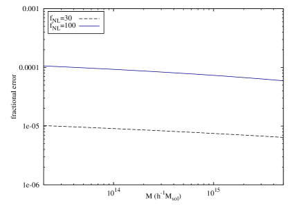
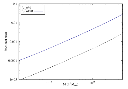
In the r.h.s of this equation we have used the saddle point approximation but have made no expansion in . By comparing the numerical integration of the l.h.s. with the expression on the r.h.s. (panel (a) of Fig. 7), one can see that the errors introduced by the saddle point approximation are indeed of order as indicated by (D.6). On the other hand, one can use the numerical integration of the left hand side of this equation and compare it with the approximation (D.5) (panel (b) of Fig. 7), to see that the biggest error is of order induced by the fact that we perform a perturbative expansion in . Notice that here we considered only the leading order in and ignored unequal time correlators, while in the main text we present a result which is more precise (to next to leading order in ) and complete (using the excursion set formalism rigorously).
References
- [1] N. Dalal, O. Dore, D. Huterer and A. Shirokov, “The imprints of primordial non-Gaussianities on large-scale structure: scale dependent bias and abundance of virialized objects,” Phys. Rev. D 77 (2008) 123514 [arXiv:0710.4560 [astro-ph]].
- [2] S. Matarrese and L. Verde, “The effect of primordial non-Gaussianity on halo bias,” Astrophys. J. 677 (2008) L77 [arXiv:0801.4826 [astro-ph]].
- [3] A. Slosar, C. Hirata, U. Seljak, S. Ho and N. Padmanabhan, “Constraints on local primordial non-Gaussianity from large scale structure,” JCAP 0808 (2008) 031 [arXiv:0805.3580 [astro-ph]].
- [4] E. Komatsu et al., “Seven-Year Wilkinson Microwave Anisotropy Probe (WMAP) Observations: Cosmological Interpretation,” arXiv:1001.4538 [astro-ph.CO].
- [5] B. Sartoris, S. Borgani, C. Fedeli, S. Matarrese, L. Moscardini, P. Rosati and J. Weller, “The potential of X-ray cluster surveys to constrain primordial non-Gaussianity,” arXiv:1003.0841 [astro-ph.CO].
- [6] C. Carbone, L. Verde and S. Matarrese, “Non-Gaussian halo bias and future galaxy surveys,” Astrophys. J. 684, L1 (2008) [arXiv:0806.1950 [astro-ph]].
- [7] C. Carbone, O. Mena and L. Verde, “Cosmological Parameters Degeneracies and Non-Gaussian Halo Bias,” JCAP 1007, 020 (2010) [arXiv:1003.0456 [astro-ph.CO]].
- [8] C. Cunha, D. Huterer and O. Dore, “Primordial non-Gaussianity from the covariance of galaxy cluster counts,” arXiv:1003.2416 [astro-ph.CO].
- [9] E. Sefusatti, “1-loop Perturbative Corrections to the Matter and Galaxy Bispectrum with non-Gaussian Initial Conditions,” Phys. Rev. D 80 (2009) 123002 [arXiv:0905.0717 [astro-ph.CO]].
- [10] R. Jimenez and L. Verde, “Implications for Primordial Non-Gaussianity () from weak lensing masses of high-z galaxy clusters,” Phys. Rev. D 80, 127302 (2009) [arXiv:0909.0403 [astro-ph.CO]].
- [11] L. Verde, “Non-Gaussianity from Large-Scale Structure Surveys,” arXiv:1001.5217 [astro-ph.CO].
- [12] V. Desjacques and U. Seljak, “Primordial non-Gaussianity from the large scale structure,” arXiv:1003.5020 [astro-ph.CO].
- [13] J. E. Gunn and J. R. I. Gott, “On the infall of matter into cluster of galaxies and some effects on their evolution,” Astrophys. J. 176, 1 (1972).
- [14] W. H. Press and P. Schechter, “Formation of galaxies and clusters of galaxies by selfsimilar gravitational condensation,” Astrophys. J. 187, 425 (1974).
- [15] J. R. Bond, S. Cole, G. Efstathiou and N. Kaiser, “Excursion set mass functions for hierarchical Gaussian fluctuations,” Astrophys. J. 379, 440 (1991).
- [16] S. Matarrese, L. Verde and R. Jimenez, “The abundance of high-redshift objects as a probe of non-Gaussian initial conditions,” Astrophys. J. 541 (2000) 10 [arXiv:astro-ph/0001366].
- [17] M. LoVerde, A. Miller, S. Shandera and L. Verde, “Effects of Scale-Dependent Non-Gaussianity on Cosmological Structures,” JCAP 0804 (2008) 014 [arXiv:0711.4126 [astro-ph]].
- [18] R. K. Sheth and G. Tormen, “An Excursion Set Model Of Hierarchical Clustering : Ellipsoidal Collapse And The Moving Barrier,” Mon. Not. Roy. Astron. Soc. 329, 61 (2002) [arXiv:astro-ph/0105113].
- [19] M. Maggiore and A. Riotto, “The Halo Mass Function from the Excursion Set Method. I. First principle derivation for the non-Markovian case of Gaussian fluctuations and generic filter,” arXiv:0903.1249 [astro-ph.CO].
- [20] M. Maggiore and A. Riotto, “The halo mass function from the excursion set method. II. The diffusing barrier,” arXiv:0903.1250 [astro-ph.CO].
- [21] M. Maggiore and A. Riotto, “The halo mass function from the excursion set method. III. First principle derivation for non-Gaussian theories,” arXiv:0903.1251 [astro-ph.CO].
- [22] P. Valageas, “Mass function and bias of dark matter halos for non-Gaussian initial conditions,” arXiv:0906.1042 [astro-ph.CO].
- [23] J. M. Bardeen, J. R. Bond, N. Kaiser and A. S. Szalay, “The Statistics Of Peaks Of Gaussian Random Fields,” Astrophys. J. 304, 15 (1986).
- [24] R. K. Sheth, H. J. Mo and G. Tormen, “Ellipsoidal collapse and an improved model for the number and spatial distribution of dark matter haloes,” Mon. Not. Roy. Astron. Soc. 323, 1 (2001) [arXiv:astro-ph/9907024].
- [25] T. Y. Lam and R. K. Sheth, “Halo abundances in the model,” arXiv:0905.1702 [astro-ph.CO].
- [26] N. Sugiyama, “Cosmic background anistropies in CDM cosmology,” Astrophys. J. Suppl. 100, 281 (1995) [arXiv:astro-ph/9412025].
- [27] U. Seljak and M. Zaldarriaga, “A Line of Sight Approach to Cosmic Microwave Background Anisotropies,” Astrophys. J. 469 (1996) 437 [arXiv:astro-ph/9603033].
- [28] A. Lewis, A. Challinor and A. Lasenby, “Efficient Computation of CMB anisotropies in closed FRW models,” Astrophys. J. 538 (2000) 473 [arXiv:astro-ph/9911177].
- [29] D. Babich, P. Creminelli and M. Zaldarriaga, “The shape of non-Gaussianities,” JCAP 0408 (2004) 009 [arXiv:astro-ph/0405356].
- [30] D. H. Lyth, C. Ungarelli and D. Wands, “The primordial density perturbation in the curvaton scenario,” Phys. Rev. D 67 (2003) 023503 [arXiv:astro-ph/0208055].
- [31] N. Bartolo, S. Matarrese and A. Riotto, “On non-Gaussianity in the curvaton scenario,” Phys. Rev. D 69 (2004) 043503 [arXiv:hep-ph/0309033].
- [32] G. Dvali, A. Gruzinov and M. Zaldarriaga, “A new mechanism for generating density perturbations from inflation,” Phys. Rev. D 69 (2004) 023505 [arXiv:astro-ph/0303591].
- [33] M. Alishahiha, E. Silverstein and D. Tong, “DBI in the sky,” Phys. Rev. D 70, 123505 (2004) [arXiv:hep-th/0404084].
- [34] N. Arkani-Hamed, P. Creminelli, S. Mukohyama and M. Zaldarriaga, “Ghost Inflation,” JCAP 0404, 001 (2004) [arXiv:hep-th/0312100].
- [35] P. Creminelli, “On non-Gaussianities in single-field inflation,” JCAP 0310, 003 (2003) [arXiv:astro-ph/0306122].
- [36] P. Creminelli, A. Nicolis, L. Senatore, M. Tegmark and M. Zaldarriaga, “Limits on non-Gaussianities from WMAP data,” JCAP 0605 (2006) 004 [arXiv:astro-ph/0509029].
- [37] J. Zinn-Justin, “Quantum field theory and critical phenomena,” Int. Ser. Monogr. Phys. 113 (2002) 1.
- [38] S. Chandrasekhar, “Stochastic problems in physics and astronomy,” Rev. Mod. Phys. 15, 1 (1943).
- [39] T. Giannantonio and C. Porciani, “Structure formation from non-Gaussian initial conditions: multivariate biasing, statistics, and comparison with N-body simulations,” arXiv:0911.0017 [astro-ph.CO].
- [40] C. Carbone et al., “The properties of the dark matter halo distribution in non-Gaussian scenarios,” Nucl. Phys. Proc. Suppl. 194, 22 (2009).
- [41] F. Bernardeau, S. Colombi, E. Gaztanaga and R. Scoccimarro, “Large-scale structure of the universe and cosmological perturbation theory,” Phys. Rept. 367, 1 (2002) [arXiv:astro-ph/0112551].
- [42] B. Robertson, A. Kravtsov, J. Tinker and A. Zentner, “Collapse Barriers and Halo Abundance: Testing the Excursion Set Ansatz,” Astrophys. J. 696 (2009) 636 [arXiv:0812.3148 [astro-ph]].
- [43] R. K. Sheth and R. van de Weygaert, “A hierarchy of voids: Much ado about nothing,” Mon. Not. Roy. Astron. Soc. 350, 517 (2004) [arXiv:astro-ph/0311260].
- [44] M. Kamionkowski, L. Verde and R. Jimenez, “The Void Abundance with Non-Gaussian Primordial Perturbations,” JCAP 0901, 010 (2009) [arXiv:0809.0506 [astro-ph]].
- [45] A. Erdélyi, “Asymptotic Expansions,” New York, NY: Dover (1956) 108pp.