Non-classical correlations in non-Markovian continuous variable systems

Abstract

We consider two identical and non-interacting harmonic oscillators coupled to either two independent bosonic baths or to a common bosonic bath. Under the only assumption of weak coupling, we analyze in details the non-Markovian short time-scale evolution of intensity correlations, entanglement and quantum discord for initial two-mode squeezed-thermal vacuum states. In the independent reservoirs case we observe the detrimental effect of the environment for all these quantities and we establish a hierarchy for their robustness against the environmental noise. In the common reservoir case, for initial uncorrelated states, we find that only quantum discord can be created via interaction with the bath, while entanglement and sub shot noise intensity correlations remain absent.

I Introduction

Quantum correlations have been the subject of intensive studies in the last two decades, mainly due to the general belief that they are a fundamental resource for quantum information processing tasks. Perhaps, the first rigorous attempt to address the classification of quantum correlation from an information viewpoint has been put forward by Werner Wer , who introduced an operational definition of quantum entanglement as the property of states that cannot be prepared by local operations and classical communication between the two parties. One might have thought that such classical information exchange could not bring any quantum character to the correlations in the state. In this sense separability has often been regarded as a synonymous of classicality of correlations. However, it has been shown recently OllZur ; HenVed that this is not the case, and a measure of correlations – quantum discord – has been introduced as the mismatch between two quantum analogues of classically equivalent expressions of the mutual information. For pure entangled states quantum discord coincides with the entropy of entanglement. However, quantum discord can be different from zero also for some (mixed) separable state. In other words, classical communication can give rise to quantum correlations due to the existence of non orthogonal quantum states. Quantum discord, therefore, captures quantum correlations more general than entanglement. Separable mixed states having nonzero quantum discord have been proven to provide computational speed up in some quantum algorithms DatCav ; LanWhi compared to their classical counterpart. In addition, the vanishing of quantum discord between two systems has been shown to be a requirement for the complete positivity of the reduced subsystem dynamics Lid09 .

The definition of quantum discord involves an optimization problem that, in general, can be tackled only for very simple systems. Even in the simplest bipartite system, i.e., a system of two qubits, an analytic expression for the discord for the most general two-qubits state does not exist. The optimization problem has been indeed only recently solved for the subset of states which are unitary locally equivalent to the so-called X-states Luo ; Ali but remains unsolved for more general states. For this reason the dynamics of the discord in presence of the environment has been up to now studied only for very simple finite-dimensional systems. In the case of two qubits, e.g., both the Markovian and the non-Markovian time evolution of quantum correlations have been investigated MarDisc ; NMDisc1 ; NMDisc2 ; NMDisc3 and it has been shown that discord and entanglement behave differently under the effect of the environment. In particular, the phenomenon of entanglement sudden death YuEbe , i.e., the complete loss of entanglement after a finite time, does not occur for quantum discord, which instead disappears only asymptotically MarDisc . Remarkably, for two-qubits systems in presence of nondissipative noise, the discord may remain constant in time for very long time intervals, providing the first evidence of a quantum property that is completely unaffected by the environmental noise for very long times Laura . The sudden transition from classical to quantum decoherence, associated to the constant discord phenomenon has been recently observed experimentally in a quantum optical set up NatComm .

In this paper we present a detailed analysis of the time evolution of quantum discord for a more involved bipartite system, namely a system consisting of two non interacting harmonic oscillators initially prepared in a thermal twin beam (TWB) state. The analytic formula for the quantum discord for generic bimodal Gaussian states has been discovered only very recently Matt ; DaAde . We use such definition to evaluate how the quantum correlations evolve in presence of both independent and common bosonic thermal reservoirs.

The system we are going to analyze have an immediate application in a quantum optical setting where it may be implemented by parametric downconversion (PDC), which has been addressed as a convenient and feasible setting to visualize the evolution of quantum correlations DBA07 ; ss07 . In turn, the pair of field modes obtained from thermally seeded PDC is as a convenient physical system to analyze the quantum-classical transition in the continuous variable regime. This scheme have been already investigated in ghost- imaging/diffraction experiments DBA07 , where it has been shown that both entanglement and intensity correlations may be tuned upon changing the intensities of the seeds DBA07 ; ss07 . In this framework, besides fundamental quantities like entanglement and quantum discord, we will also evaluate a more operational quantity as the degree of correlations between the intensities of the two beams exiting the noisy channel. The shot-noise limit (SNL) in a photodetection process is defined as the lowest level of noise that can be achieved by using semiclassical states of light SNL , that is Glauber coherent states. On the other hand, when a noise level below the SNL is observed, we have a genuine nonclassical effect. For a two-mode system if one measures the photon number of the two beams and evaluates the difference photocurrent the SNL is the lower bound to the fluctuations that is achievable with classically coherent beams and a noise level below the SNL indicates the presence of nonclassical correlations between the beams.

We consider the case in which system and environment are weakly coupled but we do not perform the Markov approximation so our results also described the initial short time correlations between the system and the reservoir. The lifetime of such correlations depends on the structure of the environment. When the spectral density of the environment changes significantly for frequencies close to the system characteristic frequency, the correlations between system and reservoir persist for a longer time and non-Markovian approaches are necessary.

The dynamics of entanglement in such structured reservoirs has been studied in both the common PraBer ; PazRon and the independent reservoir scenario PraBer ; IndepRes ; VasMan . Here we compare the time evolution of the discord with the one of both the entanglement and the intensity correlations. In the case of independent reservoirs, we can establish a hierarchy of nonclassicality markers in terms of their robustness against the destructive action of the environment. In the common reservoir scenario we find that if the initial state does not possess quantum correlations, i.e., all three markers of nonclassicality here considered have initially zero value, as time passes the interaction with the common reservoir can create quantum discord between the two system oscillators. Entanglement and nonclassical intensity correlations, however, cannot be created by the common reservoir in the weak coupling limit here studied. Finally, we analyze how the quantum discord behaves as a function of the initial thermal component of the TWB state. We discover that this quantity influences the rate of change of the discord in both the independent and the common reservoir cases.

The paper is structured as follows. In Sec. II we present the microscopic physical models for the system and the reservoir. In Sec. III we introduce the three markers of nonclassicality and, in particular, of nonclassical correlations considered in this paper: intensity correlations, entanglement and discord. Sec. IV investigates the dynamics of the markers in presence of common or independent reservoirs. Finally, Sec. V closes the paper and draws some concluding remark.

II Physical models

In this section we introduce a physical model widely used in the description of the non-Markovian dynamics of CV quantum channels. The main system is made of a pair of identical non-interacting harmonic oscillators of frequency $\omega_{0}$ and unit mass. The free Hamiltonian reads

$$\hat{H}_{0}=\hat{H}^{0}_{1}+\hat{H}^{0}_{2}=\frac{1}{2}\sum_{j=1,2}(\hat{P}_{j}^{2}+\omega_{0}^{2}\hat{X}_{j}^{2}),$$ (1)

where $\hat{P}_{j}=\frac{1}{i\sqrt{2}}(\hat{a}_{j}-\hat{a}_{j}^{\dagger})$ and $\hat{X}_{j}=\frac{1}{\sqrt{2}}(\hat{a}_{j}+\hat{a}_{j}^{\dagger})$ are the momentum and position operators, respectively, and $\hat{a}_{j}$ the field operator of the harmonic oscillators (the index $j=1,2$ labels the oscillators). Additionally, we suppose that the harmonic oscillators interact with an external environment. In the following we introduce two different interaction models.

II.1 Independent reservoirs

The first model consists of an external environment made of two independent bosonic baths with free Hamiltonian

$$\hat{H}_{B}=\sum_{j,k}\biggl{(}\frac{\hat{\Pi}_{jk}^{2}}{2m_{jk}}+\frac{m_{jk}w_{jk}^{2}\hat{Q}_{jk}^{2}}{2}\biggl{)}.$$ (2)

The index $j=1,2$ labels the bath, and $k$ runs over all the bath modes. The $\hat{\Pi}_{jk}$ ($\hat{Q}_{jk}$) are the momentum (position) operators, while $w_{jk}$ and $m_{jk}$ are the frequencies and masses associated to each bosonic mode.

Each system oscillator interacts with its own bosonic bath (same index $j$) through a position-position coupling described by the following interaction Hamiltonian

$$\begin{split}&\hat{H}_{I}=\alpha\sum_{j,k}\gamma_{jk}\hat{X}_{j}\hat{Q}_{jk},\end{split}$$ (3)

where $\gamma_{jk}$ are the coupling constants between the $j$-th oscillator and the $k$-th mode of its bath and $\alpha$ is a dimensionless coupling constant. For the sake of simplicity hitherto we assume that the baths have the same spectral structure and are equally coupled to the oscillators.

The reduced dynamics of the two oscillators in the case of stationary reservoirs is described by the following exact time-local master equation HuPaZa

$$\dot{\varrho}(t)= \sum_{j}\frac{1}{i\hbar}[\hat{H}_{j}^{0},\varrho(t)]-\Delta(t)[\hat{X}_{j},[\hat{X}_{j},\varrho(t)]]$$

$$+\Pi(t)[\hat{X}_{j},[\hat{P}_{j},\varrho(t)]]+\frac{i}{2}r(t)[\hat{X}_{j}^{2},\varrho(t)]$$

$$-i\gamma(t)[\hat{X}_{j},\{\hat{P}_{j},\varrho(t)\}],$$ (4)

where $\varrho(t)$ is the reduced density operator of the oscillators and $\hat{H}_{j}^{0}$ is the free Hamiltonian of the $j$-th oscillator. The time dependent coefficients, describing diffusion ($\Delta(t)$, $\Pi(t)$), damping ($\gamma(t)$) and free frequency renormalization($r(t)$) processes, can be expressed as power series in the system-reservoir coupling constant $\alpha$. In the weak coupling limit we can stop the expansion to second order in $\alpha$ and obtain analytic solutions for the coefficients. We provide their expressions in the Appendix for high temperature reservoirs characterized by an Ohmic spectral density with Lorentz-Drude cutoff $J(\omega)=\frac{\omega_{c}^{2}}{\pi}\frac{\omega}{\omega^{2}+\omega_{c}^{2}}$.

Using the characteristic function approach the solution of (4) in the weak coupling limit is given by Intra

$$\chi_{t}(\Lambda)= \mbox{}\exp\{-\Lambda^{T}[\bar{\mathbf{W}}(t)\oplus\bar{\mathbf{W}}(t)]\Lambda\}$$

$$\times\chi_{0}(e^{-\Gamma(t)/2}[\mathbf{R}^{-1}(t)\oplus\mathbf{R}^{-1}(t)]\Lambda),$$ (5)

where $\chi_{t}(\Lambda)$ is the characteristic function at time $t$, $\chi_{0}$ is the characteristic function at the initial time $t=0$, $\Lambda=(x_{1},p_{1},x_{2},p_{2})^{T}$ is the two-dimensional phase space variables vector, $\Gamma(t)=2\int_{0}^{t}\gamma(t^{\prime})dt^{\prime}$, and $\bar{\mathbf{W}}(t)$ and $\mathbf{R}(t)$ are $2\times 2$ matrices whose expression is also given in the Appendix.

The interaction between oscillators and baths is bilinear in position and momentum, thus it induces a Gaussian evolution. This is of great importance because, as we will see, analytic expressions for quantum correlations can be obtained only in the case of Gaussian states.

The characteristic function of a Gaussian state with zero mean depends only on the expression of the covariance matrix $\sigma$, whose elements are defined as $\sigma_{ij}=\langle\{\hat{\Lambda}_{i},\hat{\Lambda}_{j}\}\rangle/2-\langle\hat{\Lambda}_{i}\rangle\langle\hat{\Lambda}_{j}\rangle$, where $\hat{\Lambda}\equiv(\hat{X}_{1},\hat{P}_{1},\hat{X}_{2},\hat{P}_{2})$ and $\langle\cdot\rangle$ indicates the mean value over the state,

$$\chi_{0}(\Lambda)=\exp\biggl{\{}-\frac{1}{2}\Lambda^{T}\sigma(0)\Lambda\biggl{\}}.$$ (6)

Using Eqs. (5) and (6) we get the evolution of the covariance matrix under the action of the two independent reservoirs

$$\begin{split}\sigma(t)=&e^{-\Gamma(t)}[\mathbf{R}(t)\oplus\mathbf{R}(t)]\sigma(0)[\mathbf{R}(t)\oplus\mathbf{R}(t)]^{-1}\\ &+2[\bar{\mathbf{W}}(t)\oplus\bar{\mathbf{W}}(t)].\end{split}$$ (7)

The solution in the case of an initial symmetric covariance matrix in its normal form is

$$\sigma(0)=\left(\begin{array}[]{cc}\mathbf{A_{0}}&\mathbf{C_{0}}\\ \mathbf{C_{0}}&\mathbf{A_{0}}\\ \end{array}\right)\Rightarrow\sigma(t)=\left(\begin{array}[]{cc}\mathbf{A^{ind}_{t}}&\mathbf{C^{ind}_{t}}\\ \mathbf{C^{ind}_{t}}&\mathbf{A^{ind}_{t}}\\ \end{array}\right),$$ (8)

with $\mathbf{A_{0}}=a\,{\mathbbm{1}}$, $\mathbf{C_{0}}={\rm diag}(c_{1},c_{2})$, $a>0$ and $c_{1}$, $c_{2}$ real numbers, and $\mathbbm{1}$ the $2\times 2$ identity matrix (note that $\mathbf{C_{0}}$ and $\mathbf{C^{ind}_{t}}$ are symmetric matrices). The analytic expression of the matrices $\mathbf{A^{ind}_{t}}$ and $\mathbf{C^{ind}_{t}}$ is given in the Appendix.

II.2 Common reservoir

In the second example of system-environment interaction model, we consider a common bosonic bath, and look at the case in which both system oscillators interact with it symmetrically. The Hamiltonian reads

$$\begin{split}&\hat{H}_{B}+\hat{H}_{I}=\sum_{k}\biggl{(}\frac{\hat{\Pi}_{k}^{2}}{2m_{k}}+\frac{m_{k}w_{k}^{2}\hat{Q}_{k}^{2}}{2}\biggl{)}+\alpha\sum_{j,k}\gamma_{k}\hat{X}_{j}\hat{Q}_{k}.\end{split}$$ (9)

In order to write the reduced dynamics solution $\varrho(t)$, we first apply a canonical transformation to the Hamiltonian following the lines of PazRon . We define new position $\hat{X}_{\pm}=(\hat{X}_{1}\pm\hat{X}_{2})/\sqrt{2}$ and momentum $\hat{P}_{\pm}=(\hat{P}_{1}\pm\hat{P}_{2})/\sqrt{2}$ operators for the system. Under this transformation the total Hamiltonian becomes

$$H_{0} =\frac{\hat{P}_{+}^{2}+\hat{P}_{-}^{2}}{2}+\frac{\omega_{0}^{2}}{2}(\hat{X}_{+}^{2}+\hat{X}_{-}^{2})$$ (10a)

$$H_{R} =\sum_{k}\biggl{(}\frac{\hat{\Pi}_{k}^{2}}{2m_{k}}+\frac{m_{k}w_{k}^{2}\hat{Q}_{k}^{2}}{2}\biggl{)}$$ (10b)

$$H_{I} =\alpha\sqrt{2}\hat{X}_{+}\sum_{k}\gamma_{k}\hat{Q}_{k}$$ (10c)

In this picture only one oscillator interacts with the bath through a position-position coupling, the other evolving freely. It follows that the master equation for the reduced state $\tilde{\varrho}(t)$ in the new picture becomes

$$\dot{\tilde{\varrho}}(t)= \frac{1}{i\hbar}[(\hat{H}_{-}^{0}+\hat{H}_{+}^{0}),\tilde{\varrho}(t)]-\sqrt{2}\Delta(t)[\hat{X}_{+},[\hat{X}_{+},\tilde{\varrho}(t)]]$$

$$+\sqrt{2}\Pi(t)[\hat{X}_{+},[\hat{P}_{+},\tilde{\varrho}(t)]]+\frac{i}{\sqrt{2}}r(t)[\hat{X}_{+}^{2},\tilde{\varrho}(t)]$$

$$-i\sqrt{2}\gamma(t)[\hat{X}_{+},\{\hat{P}_{+},\tilde{\varrho}(t)\}],$$ (11)

This is of the same form of (4), except for the fact that only one effective oscillator is coupled to the environment. The dynamics in terms of the characteristic function is then

$$\tilde{\chi}_{t}(\Lambda_{\pm})= \exp\{-\Lambda^{T}_{\pm}[\sqrt{2}\bar{\mathbf{W}}(t)\oplus\mathbf{0}]\Lambda_{\pm}\}$$

$$\times\tilde{\chi}_{0}([e^{-\frac{\Gamma(t)}{\sqrt{2}}}\mathbf{R}^{-1}(t)\oplus\mathbf{R}^{-1}(t)]\Lambda_{\pm}),$$ (12)

with $\Lambda_{\pm}=(x_{+},p_{+},x_{-},p_{-})^{T}$ and $\mathbf{0}$ being the $2\times 2$ zero matrix. Equivalently, the associated covariance matrix $\tilde{\sigma}(t)$ evolves as

$$\tilde{\sigma}(t)= \left[e^{-\frac{\Gamma(t)}{\sqrt{2}}}\mathbf{R}(t)\oplus\mathbf{R}(t)\right]\tilde{\sigma}(0)\left[e^{-\frac{\Gamma(t)}{\sqrt{2}}}\mathbf{R}(t)\oplus\mathbf{R}(t)\right]^{-1}$$

$$+2\sqrt{2}[\bar{\mathbf{W}}(t)\oplus\mathbf{0}].$$ (13)

As in the previous case an initial Gaussian state will maintain its character during the time evolution. Indeed, the canonical transformation, its inverse and the dynamical evolution are all Gaussian operations.

Given the initial covariance matrix $\sigma(0)$, applying the transformations and using Eqs. (12) and (13) we get

$$\sigma(0)=\left(\begin{array}[]{cc}\mathbf{A_{0}}&\mathbf{C_{0}}\\ \mathbf{C_{0}}&\mathbf{A_{0}}\\ \end{array}\right)\Rightarrow\sigma(t)=\left(\begin{array}[]{cc}\mathbf{A^{com}_{t}}&\mathbf{C^{com}_{t}}\\ \mathbf{C^{com}_{t}}&\mathbf{A^{com}_{t}}\\ \end{array}\right),$$ (14)

with $\mathbf{C^{com}_{t}}$ symmetric matrix. Details of the solution are still given in the Appendix.

III Non-classical Correlations

In the last decades there has been a growing interest in the issue of identifying and possibly quantifying the quantumness of states of a given physical system. One of the reasons is that states possessing quantum features may be useful for certain quantum information and computation protocols, or in the field of precision measurements, enhancing computation and measurements efficiencies.

In the case of bipartite (or in general multipartite) systems the interest is directed not only towards the quantumness of the state itself, but also towards the quantumness of correlations between the different parts. In this paper we provide new insight on this issue by comparing different markers of quantumness of states and correlations. In particular we are interested in studying how non-Markovian dynamical evolutions affect these quantities in the context of two mode continuous variable systems. In the following we introduce the well-known concepts of intensity correlations and entanglement in CV systems as well as the recently introduced quantum discord for Gaussian states.

III.1 Intensity correlations

Firstly we consider the intensity correlations marker $\mathbf{I}_{\rm corr}$, which is related to the measurement of the two light beams intensities, i.e., $\langle\hat{n}_{1}\rangle$ and $\langle\hat{n}_{2}\rangle$, with $\hat{n}_{i}=(\hat{X}_{i}^{2}+\hat{P}_{i}^{2})/2$ being the number operator of the $i$-th mode, and thus feasible with current technology. More precisely, the intensity correlations marker is defined as DBA07 ; Icorr:brida

$$\mathbf{I}_{\rm corr}=1-\frac{\langle\Delta\hat{I}_{-}^{2}\rangle}{\langle\hat{n}_{1}+\hat{n}_{2}\rangle},$$ (15)

and is based on the measurement of the operator $\hat{I}_{-}=\hat{n}_{1}-\hat{n}_{2}$, that is the difference between the intensities of the two light modes, whose variance $\langle\Delta\hat{I}_{-}^{2}\rangle$ may also be written as

$$\langle\Delta\hat{I}_{-}^{2}\rangle =\langle\hat{I}_{-}^{2}\rangle-\langle\hat{I}_{-}\rangle^{2},$$ (16)

$$=\langle\Delta\hat{n}_{1}^{2}\rangle+\langle\Delta\hat{n}_{2}^{2}\rangle-2\langle\hat{n}_{1}\rangle\langle\hat{n}_{2}\rangle\,g^{(2)}(\hat{n}_{1},\hat{n}_{2}),$$ (17)

where we introduced the second-order correlation function

$$g^{(2)}(\hat{n}_{1},\hat{n}_{2})=\frac{\langle\hat{n}_{1}\hat{n}_{2}\rangle}{\langle\hat{n}_{1}\rangle\langle\hat{n}_{2}\rangle}-1.$$ (18)

In the case of products of coherent states we have $\mathbf{I}_{\rm corr}=0$, which defines the shot-noise limit (SNL) for this particular detection process, that is the lowest level of noise that can be obtained by using the semiclassical states of light, i.e., the coherent states. On the other hand, when

$$0<\mathbf{I}_{\rm corr}\leq 1,$$ (19)

the fluctuations on the intensity correlations are below the SNL, indicating genuine non-classical features in the state of the system. It is worth stressing that intensity correlations below the SNL can be observed also for product states, for example in the presence of local squeezing. Hence, this feature is not necessary related to the quantumness of correlations among different parts of our bipartite system, but rather to the quantumness of the overall state itself ferr:prep .

For a Gaussian state with zero mean value, $\mathbf{I}_{\rm corr}$ depends only on the corresponding covariance matrix $\sigma$ and, in the case of symmetric Gaussian states, reads

$$\mathbf{I}_{\rm corr}=1-\frac{\sigma^{2}_{11}+\sigma^{2}_{22}+2\sigma_{13}^{2}-\sigma_{14}^{2}-\sigma_{23}^{2}-\sigma_{24}^{2}-\frac{1}{2}}{\sigma_{11}+\sigma_{22}-1},$$ (20)

where $\sigma_{ij}$ are the covariance matrix entries.

III.2 Entanglement

Entanglement dynamics in dissipative bipartite continuous variable domain has been object of interest and numerous studies in recent years PraBer ; PazRon ; IndepRes ; VasMan . Though there exist separability criteria and entanglement measures for a bipartite Gaussian state $\varrho$ (see, e.g., Simon ; EntFor ; buono:JOSAB:10 ), in this paper we study the entanglement dynamics by focusing on the logarithmic negativity defined as Nega

$$\mathcal{N}(\varrho)=\max\{0,-\log(2\tilde{\nu}_{-})\},$$ (21)

with $\tilde{\nu}_{-}$ being the minimum symplectic eigenvalue of the partially transpose ($\mathbf{PT}$) covariance matrix of the system, namely, $\sigma^{\rm PT}={\bm{\Delta}}\sigma{\bm{\Delta}}$ with ${\bm{\Delta}}=\hbox{diag}(1,-1,1,-1)$. It is worth to note that $\mathcal{N}(\varrho)>0$ if and only if $\tilde{\nu}_{-}<1/2$, that is if and only if the state $\varrho$ is entangled: of course, the condition $\tilde{\nu}_{-}<1/2$ is a necessary and sufficient condition for a bipartite Gaussian state to be non separable Simon .

III.3 Quantum Discord

The total amount of correlations in a bipartite quantum system having density operator $\varrho$ is quantified by the quantum version of the mutual information

$$\mathcal{I}(\varrho)=S(\varrho_{1})+S(\varrho_{2})-S(\varrho),$$ (22)

where $S(\cdot)$ is the Von Neumann entropy, and $\varrho_{1(2)}=\hbox{Tr}_{2(1)}[\varrho]$. Usually the total correlations are divided in a quantum part, known as quantum discord $\mathcal{D}(\varrho)$, and a classical part $\mathcal{C}(\varrho)$. The classical correlations are defined as the maximum amount of information we can gain on one part of the system by locally measuring the other subsystem HenVed ,

$$\begin{split}\mathcal{C}(\varrho)=\max_{\Pi_{i}}\bigl{\{}S(\varrho_{1})-\sum_{i}p_{i}S(\varrho^{\Pi_{i}}_{1|2})\bigl{\}},\end{split}$$ (23)

where $\varrho^{\Pi_{i}}_{1|2}=\mbox{Tr}_{2}(\varrho\openone\otimes\Pi_{i})$ is the post measurement state in which system $1$ is left when the result $i$ occurs in a measurement of system $2$ with probability $p_{i}=\mbox{Tr}_{1\,2}(\varrho\openone\otimes\Pi_{i})$. The maximum is taken over the all positive operator valued measures $\{\Pi_{i}\}$ (POVM), $\sum_{i}\Pi_{i}=\openone$ performable on one subsystem. Classical correlations are thus obtained in correspondence of the POVM that minimizes the conditional entropy $\sum_{i}p_{i}S(\varrho^{\Pi_{i}}_{1|2})$ i.e., that allows one to obtain the highest amount of information on the state of system $1$. The above definition is in general non symmetric with respect to the interchange of the subsystems. In our case however, due to our specific choice of the system’s initial states (see below) and to the symmetry of the coupling with the bath, (23) turns out to be symmetric during the entire evolution; therefore no specific indication of the subsystem measured will be needed. The quantum discord is then defined as the difference between the total correlations and the classical correlations

$$\begin{split}&\mathcal{D}(\varrho)=\mathcal{I}(\varrho)-\mathcal{C}(\varrho).\end{split}$$ (24)

A peculiar property of quantum discord is that it can be nonzero even if the state is separable. This is an indication of the fact that entanglement is not the only source of quantum correlations. Recently examples of quantum computational algorithms showing a speedup with respect to the classical counterparts, also in the absence of entanglement, have been presented DatCav ; LanWhi . It is believed that the presence of quantum correlations other-than-entanglement is responsible for this feature. In this sense it is important to study how the quantum discord evolves in presence of the external environments, comparing, e.g., its behavior with the behavior of entanglement. In the following we answer to this question for Gaussian states of CV systems.

To evaluate the total quantum correlations we use a recently developed expression valid only for Gaussian states Matt ; DaAde . Given the block form of the covariance matrix $\sigma(t)$ (8) and (14), in the symmetric case, the Gaussian quantum discord is defined as

$$\mathcal{D}(\varrho)=f\left(\sqrt{{\rm det}\mathbf{A_{t}}}\right)+f\left(\sqrt{{\rm det}\mathbf{\tau}}\right)-f(n_{+})-f(n_{-}),$$ (25)

where $f(x)=(x+\frac{1}{2})\ln(x+\frac{1}{2})-(x-\frac{1}{2})\ln(x-\frac{1}{2})$, $n_{\pm}$ are the symplectic eigenvalues of the covariance matrix and

$$\tau=\mathbf{A_{t}}-\mathbf{C_{t}}(\mathbf{A_{t}}+\sigma_{M})^{-1}\mathbf{C_{t}}^{T},$$ (26)

is the covariance matrix of the state of the system $A$ after the generalized Gaussian measurement on the system $B$, described by the covariance matrix

$$\sigma_{M}=\frac{\cosh 2\rho}{2}\left(\begin{array}[]{cc}1+\tanh 2\rho\cos\phi&-\tanh 2\rho\sin\phi\\ -\tanh 2\rho\sin\phi&1-\tanh 2\rho\cos\phi\\ \end{array}\right),$$ (27)

with $\rho\geq 0$ and $0\leq\phi\leq 2\pi$. For a generic Gaussian state we must perform a minimization procedure in order to find the appropriate generalized measurement for the calculus of the quantum discord. In the case of $\mathbf{C_{t}}={\rm diag}(c,-c)$ the minimum is obtained for a completely heterodyne measurement Matt . For a generic covariance matrix in its normal form the exact expression for the discord has been evaluated in DaAde . However in our cases the time evolution of the covariance matrix is not in the normal form. Therefore to evaluate the discord it was faster to implement a numerical minimization procedure.

IV Results

In this section we study the evolution of the previously introduced markers of nonclassicality under the influence of either independent or common reservoirs, in the weak coupling regime. We limit our investigation to the case of an Ohmic spectrum with Lorentz-Drude cut-off at high temperatures focusing on the non-Markovian short time-scale. Moreover we fix hitherto the coupling constant $\alpha=0.1$ and $k_{B}T/\hbar\omega_{c}=100$, according respectively to the weak coupling and high temperature assumptions.

An important parameter in our discussion is the ratio between the cut-off frequency of the baths spectrum $\omega_{c}$ and the oscillator frequency $\omega_{0}$, namely the resonance parameter $x=\omega_{c}/\omega_{0}$. In VasMan we have studied the non-Markovian entanglement dynamics noting the existence of two dynamical regimes ($x\ll 1$ and $x\gg 1$) characterized by qualitatively and quantitatively different dynamical behaviors. Genuine non-Markovian effects occur in the $x\ll 1$ regime because the time-dependent coefficients in the Master equation attain negative values in certain time intervals. This feature leads to entanglement oscillations, which are not present in the $x\gg 1$ case. As we will see, the same conclusion is valid for the intensity correlations and the quantum discord, also in the common reservoir scenario. Moreover, in general, the dynamics for $x\ll 1$ is much slower. In the following we concentrate especially on the $x\gg 1$ regime, or linear spectrum regime, unless qualitatively different phenomena can be reported in the other regime.

Let us consider as initial states the thermal TWB states defined as

$$\varrho_{in}(r,N_{1},N_{2})=\hat{S}_{2}(r)\nu(N_{1})\otimes\nu(N_{2})\hat{S}_{2}^{{\dagger}}(r),$$ (28)

where $\nu(N)=\sum_{n}N^{n}(1+N)^{-(n+1)}\displaystyle{|n\rangle}\displaystyle{\langle n|}$ is a thermal state with $N$ average photons and $\hat{S}_{2}(r)=\exp\{r(\hat{a}_{1}^{{\dagger}}\hat{a}_{2}^{{\dagger}}-\hat{a}_{1}\hat{a}_{2})\}$ is the two-mode squeezing operator. In the symmetric case we are interested in the two thermal states are characterized by the same temperature parameter $N_{1}=N_{2}=N$, while the squeezing parameter $r$ can assume any non negative value. The covariance matrix $\sigma(0)$ of the initial state is given by

$$\mathbf{A}_{0}=\left(\begin{array}[]{cc}a&0\\ 0&a\\ \end{array}\right),\qquad\mathbf{C}_{0}=\left(\begin{array}[]{cc}c&0\\ 0&-c\\ \end{array}\right),$$ (29)

with $a=(N+1/2)\cosh(2r)$ and $c=(N+1/2)\sinh(2r)$. If $r=0$ the state is initially uncorrelated. If $r>0$ the state may be entangled or separable, depending on the value of $N$, but it will always possess non-zero quantum discord Matt .

IV.1 Independent reservoirs

Initially uncorrelated states cannot become correlated at a later time when evolving under local operations, as in the case of the independent reservoirs model. Thus we focus here on initially correlated states ($r>0$). In all the various examples we examined, we observed that the interaction with the reservoirs has a detrimental effect for all the quantumness markers introduced in the previous section. In this sense, not only the state becomes more classical but also the quantum correlations decrease.

Entanglement however behaves differently from quantum discord. Indeed entanglement can disappear after a finite time, exhibiting a sudden death and, depending on bath parameters and temperature, also exhibit partial revivals VasMan . On the contrary, in our system the quantum discord vanishes only for $t\rightarrow\infty$, a result which is independent from the value of the resonance parameter and, at least in the weak coupling limit, it is also independent from the spectral distribution and temperature regime. This is a consequence of the fact that Gaussian quantum discord is zero if and only if the Gaussian state is a product state and therefore if and only if the determinant of the $C$ matrix is zero Matt ; DaAde . This condition is never satisfied in weak coupling case for initial two-mode squeezed thermal states (see Appendix).

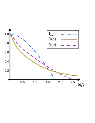
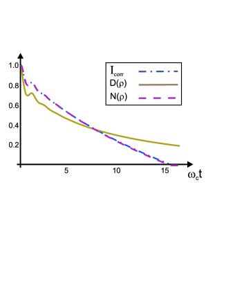
In FIG. 1 we show the behavior of $\mathbf{I}_{\rm corr}$ (only the sub-shot noise regime), $\mathcal{N}(\varrho)$ and $\mathcal{D}(\varrho)$ for initial states with $r=2$ and $N=0$ as a function of $\omega_{c}t$. Note that, in the figures we have scaled all these quantities so that their initial value coincides. In FIG. 1 (top) we choose $x=10$, while in FIG. 1 (bottom) we have $x=0.2$. The dynamics is faster when $x$ is large and it does not present oscillations typical of a non-Markovian evolution. Moreover entanglement is more robust to the detrimental effect of the environment than $\mathbf{I}_{\rm corr}$. This is valid also for $x\ll 1$, a fact that helps us to set up a hierarchy for the behavior of our quantities under the influence of the independent environment. We will see that such a classification cannot be done instead in the more complicated dynamics due to a common reservoir.

On the other hand when $x\ll 1$ non-Markovian oscillations are present in all quantum markers. Moreover, in this case, intensity correlations and entanglement go to zero at the same time, independently from the initial thermal squeezed state.

Figure 1: (Colors online) Evolution of intensity correlations marker $\mathbf{I}_{\rm corr}$ below the SNL (blue dashed line), logarithmic negativity $\mathcal{N}(\varrho)$ (red dashed line) and quantum discord $\mathcal{D}(\varrho)$ (solid yellow line) in the independent reservoir case as a function of $\omega_{c}t$. Parameters: $\alpha=0.1$, $k_{B}T/\hbar\omega_{c}=100$ and (top) $x=10$, $r=2$, $N=0$; (bottom) $x=0.2$, $r=0.5$, $N=0$.

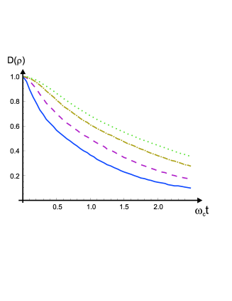
We conclude this section with an analysis of the dynamics as a function of the thermal parameter $N$ of the initial state, concentrating in particular on the dynamics of the quantum discord. In FIG. 2 we show the time evolution of $\mathcal{D}(\varrho)$ for $x=10$, $r=2$ and different values of $N=0,1,5,10$. One can clearly see that the higher is $N$ the slower is the loss rate of quantum correlations under the action of local bosonic baths. In other words, states with initially higher thermal component loose quantum correlations, as measured by the discord, more slowly than states with smaller thermal component.

Figure 2: (Colors online) Evolution of quantum discord $\mathcal{D}(\varrho)$ as a function of the scaled time $\omega_{c}t$ in the independent reservoir scenario. Parameters: $\alpha=0.1$, $k_{B}T/\hbar\omega_{c}=100$, $x=10$ and $r=2$. Different lines represent different values of the thermal parameter: $N=0$ (Solid blue line), $N=1$ (Dashed red line), $N=5$ (Dotted-dashed yellow line) and $N=10$ (Dotted green line).

IV.2 Common reservoir

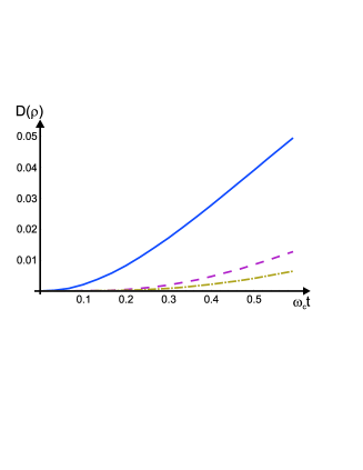
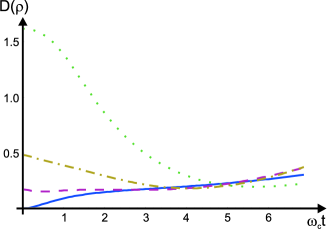
In the common reservoir case the CV system dynamics is much richer than in the independent reservoir case. Initially uncorrelated states, e.g, become in general correlated as time passes. For the class of initial Gaussian states considered in the paper, however, and in the weak coupling limit, we find that, if $r=0$, neither entanglement nor intensity correlations below the SNL are created (always $\mathbf{I}_{\rm corr}<0$ ). On the contrary, quantum discord is created by the action of the common environment and grows as time passes, for any the value of $N$ and of the resonance parameter $x$, as shown in FIG. 3 for $x=10$. This result holds also in the Markovian case PraBer . Therefore, in CV systems, the common reservoir always creates quantum correlations in the weak coupling regime.

We note that the initial value of $N$ affects the rate of change of the quantum discord similarly to the independent reservoir scenario discussed in the previous section. While there, for initial correlated states, the higher was $N$ the slower was the decrease of the discord, here, for initially uncorrelated states, the higher is $N$ the slower is the increase of the discord, as one can see from FIG. 3, in the $x=10$ case. This result holds for any value of the resonance parameter $x$.

Figure 3: (Colors online) Evolution of quantum discord $\mathcal{D}(\varrho)$ as a function of the scaled time $\omega_{c}t$ in the common reservoir scenario. Parameters: $\alpha=0.1$, $k_{B}T/\hbar\omega_{c}=100$, $x=10$ and $r=0$ (initially uncorrelated state). Different lines represent different values of the thermal parameter: $N=0$ (Solid blue line), $N=0.05$ (Dashed red line), $N=0.1$ (Dotted-dashed yellow line).

We now turn to the initially correlated case, i.e., initial states having $r>0$ and $N\geq 0$. In the common reservoir scenario a comparison between the dynamics of the three markers, as the one presented for independent reservoirs, does not provide interesting information. The reason is that it is not possible to identify a general hierarchy for the most robust quantities under the action of the environment. Indeed the dynamics is more strongly dependent on the initial state and reservoir parameters and the robustness of each of the markers changes case by case without exhibiting a general trend. Therefore we will present in the following the most interesting dynamical features of each quantity separately.

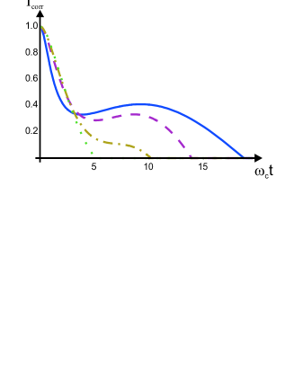
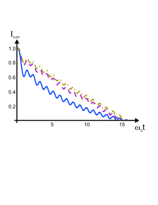
Initial states possessing intensity correlations initially below the SNL, for small values of $N$, always lose them completely in a finite time. For large $x$ (FIG. 4 (top)) and $N=0$ there are no revivals as expected in this dynamical regime. A surprising result is, however, that the larger is the initial two-mode squeezing the faster the SNL is reached. One would expect, indeed, that initial states with higher values of intensity correlations initially below the SNL maintain this quantum property for longer times than initial states having smaller values of intensity correlations initially below the SNL. An opposite result is reached in the case of small $x$ (FIG. 4 (bottom)), where the environment leads to a faster loss of intensity correlations when $r$ is smaller. In this case however the SNL limit is reached at the same time for each value of $r$ and some oscillations and revivals are present due to the non-secular terms of the solution.

Figure 4: (Colors online) Dynamics of the intensity correlations marker $\mathbf{I}_{\rm corr}$ for a common reservoir as a function of $\omega_{c}t$. Parameters: $\alpha=0.1$, $k_{B}T/\hbar\omega_{c}=100$, $N=0$, (top) $x=10$; (bottom) $x=0.3$. $r=0.5$ (Blue solid line), $r=1$ (Purple dashed line), $r=1.5$ (Yellow dot-dashed line), $r=5$ (Green dotted line).

The behavior of entanglement in these systems has been studied in detail in previous papers PraBer ; PazRon . We can however summarize the most important features. In the weak coupling regime, if there is no initial entanglement, it is not possible to create it. This has been already pointed out previously for uncorrelated initial conditions. The same conclusion holds, however, also for initially correlated states with high enough values of $N$ in the initial state. In general, for initially entangled states, in the short-time scale we can observe sudden death and revivals depending on the values of $N$, $r$ ,$x$. If the initial value of the entanglement is small, it is rather difficult to observe revivals. Some revivals can be seen in the $x\ll 1$ case, usually due to non-secular terms VasMan . When the system is initially strongly correlated entanglement sudden death and revivals can be observed as well as situations in which in the non-Markovian time scale the entanglement never goes to zero.

Finally, we consider the behavior of the quantum discord. As in the uncorrelated case, the value of $N$ in the initial state influence the rate of discord changes. High values of $N$ make the correlations more robust to the influence of the reservoir. The value of the resonance parameter $x$ does not influence the qualitative behavior of quantum discord. Small $x$ lead to a slower dynamics and presence of oscillations in the solution. So we consider as an example the case $N=0$ and $x=10$ (See. FIG. 5 ). The different curves correspond to different values of $r$. If $r$ is small (also $r=0$) the discord has an initial small value and starts to increase during the dynamics for short times. On the contrary if $r$ is large the discord has an initial high value and it decreases in time. However, independently from the value of $r$, after an initial transient time interval, all the discord curves tend to overlap. The interaction with the common bath seems to destroy the original information on the initial correlations during such transient time interval, driving the CV system towards states which have similar value of the quantum discord.

Figure 5: (Colors online) Evolution of quantum discord $\mathcal{D}(\varrho)$ as a function of the scaled time $\omega_{c}t$ in the common reservoir scenario. Parameters: $\alpha=0.1$, $k_{B}T/\hbar\omega_{c}=100$, $x=10$, $N=0$. Different lines represent different values of the squeezing parameter: $r=0$ (Solid blue line), $r=0.2$ (Dashed red line), $r=0.4$ (Dotted-dashed yellow line) and $r=1$ (Dotted green line).

V Conclusions

In this paper we have studied the time evolution of three different indicators of quantum correlations for a bipartite CV system initially prepared in a thermal TWB state and interacting with either independent reservoirs or a common reservoir at high temperature. Using a definition for the quantum discord in CV systems recently introduced in Refs Matt ; DaAde , we have calculated analytically the dynamics of such quantity under the only assumption of weak coupling between the system and the environment. Moreover, we have compared the dynamics of the discord with the dynamics of entanglement and intensity correlations.

We have demonstrated that, in the independent reservoir scenario, initially correlated thermal TWB states, more specifically states with nonzero initial discord, loose their quantum correlations slower and slower for increasing values of their initial thermal component $N$. Similarly, in the common reservoir scenario, for initially uncorrelated states having zero discord, the higher is $N$, the slower is the reservoir-mediated rate of increase of quantum discord.

A comparison between the dynamics of discord, entanglement and intensity correlations shows that, when the two system oscillators interact with independent reservoirs, initial nonclassical intensity correlations disappear faster than the initial entanglement, which in turn disappear faster than the initial discord, for $x\gg 1$. In the opposite regime $x\ll 1$, the dynamics of the intensity correlations and of the entanglement is very similar and both quantities disappear at the same finite time.

In the common reservoir scenario, we have studied whether initial states possessing zero correlations can become correlated via the action of the reservoir in the weak coupling case here considered. Our results show that only discord can be created, while entanglement and initial correlations remain zero if they are initially zero. In fact, quantum states with nonzero discord are much more common than entangled states, as demonstrated, e.g., in Ferr . In this sense we expect quantum discord to be easier to generate than entanglement.

Our results are the first attempt to characterize the time evolution of discord and intensity correlations, comparing them to the time evolution of the entanglement, in CV non-Markovian systems. Hence they provide a first step in the description of the behavior of quantum correlations and their robustness under the effect of dissipative environments. In the future we plan to investigate whether effects such as the constant discord and the sudden transition form classical to quantum decoherence Laura , recently discovered in bipartite qubits systems, may occur also in CV systems.

Appendix A The master equation coefficients

The time-dependent coefficients of the master equations (4) and (11), in the case of thermal reservoirs and at the second order in the coupling $\alpha$ are given by

$$\Delta(t) =\alpha^{2}\!\!\int_{0}^{t}\!\!ds\!\int_{0}^{+\infty}\!\!\!\!\!\!\!\!\!d\omega J(\omega)[2N(\omega)+1]\cos(\omega s)\cos(\omega_{0}s),$$ (30a)

$$\Pi(t) =\alpha^{2}\!\!\int_{0}^{t}\!\!ds\!\int_{0}^{+\infty}\!\!\!\!\!\!\!\!\!d\omega J(\omega)[2N(\omega)+1]\cos(\omega s)\sin(\omega_{0}s),$$ (30b)

$$\gamma(t) =\alpha^{2}\!\!\int_{0}^{t}\!\!ds\!\int_{0}^{+\infty}\!\!\!\!\!\!\!\!\!d\omega J(\omega)\sin(\omega s)\sin(\omega_{0}s),$$ (30c)

$$r(t) =\alpha^{2}\!\!\int_{0}^{t}\!\!ds\!\int_{0}^{+\infty}\!\!\!\!\!\!\!\!\!d\omega J(\omega)\sin(\omega s)\cos(\omega_{0}s),$$ (30d)

with $N(\omega)=[\exp(\hbar\omega/k_{B}T)-1]^{-1}$ being the mean number of photons with frequency $\omega$, while $J(\omega)$ defines the spectral distribution of the environments. For the Ohmic distribution with Lorentz-Drude cut-off in the high-T limit ($2N(\omega)+1\simeq k_{B}T/\hbar\omega$) we have

$$\Delta(t) =\frac{\alpha^{2}\omega_{0}x^{2}}{2(1+x^{2})}\frac{k_{B}T}{\hbar\omega_{c}}\{x-e^{-\tau}[x\cos(\tau/x)-\sin(\tau/x)\},$$ (31a)

$$\Pi(t) =\frac{\alpha^{2}\omega_{0}x^{2}}{2(1+x^{2})}\frac{k_{B}T}{\hbar\omega_{c}}\{1-e^{-\tau}[\cos(\tau/x)+x\sin(\tau/x)]\},$$ (31b)

$$\gamma(t) =\frac{\alpha^{2}\omega_{0}x^{2}}{2(1+x^{2})}\{1-e^{-\tau}[\cos(\tau/x)+x\sin(\tau/x)]\}.$$ (31c)

We do not provide the analytic expression of $r(t)$ because its contribution to the solution in the weak coupling limit is negligible.

Appendix B The master equation solution

The time evolution of the characteristic functions in our two decoherence models (5) and (12) contain the $2\times 2$ matrices $\mathbf{R}(t)$ and $\bar{\mathbf{W}}(t)$. Under the weak coupling assumption their expressions is

$$\mathbf{R}(t)=\left(\begin{array}[]{cc}\cos\omega_{0}t&\sin\omega_{0}t\\ -\sin\omega_{0}t&\cos\omega_{0}t\\ \end{array}\right),$$ (32)

$$\bar{\mathbf{W}}(t)=e^{-\Gamma(t)}\mathbf{R}(t)\biggl{[}\int_{0}^{t}e^{-\Gamma(s)}\mathbf{M}(s)ds\biggl{]}\mathbf{R}^{T}(t),$$ (33)

with

$$\mathbf{M}(t)=\mathbf{R}^{T}(t)\left(\begin{array}[]{cc}\Delta(t)&-\Pi(t)/2\\ -\Pi(t)/2&0\\ \end{array}\right)\mathbf{R}(t).$$ (34)

If we explicit the calculations the following functions appear

$$\Gamma(t)=2\int_{0}^{t}\gamma(s)ds,$$ (35a)

$$\Delta_{\Gamma}(t)=e^{-\Gamma(t)}\int_{0}^{t}e^{\Gamma(s)}\Delta(s)ds,$$ (35b)

$$\Delta_{co}(t)=e^{-\Gamma(t)}\int_{0}^{t}e^{\Gamma(s)}\Delta(s)\cos[2\omega_{0}(t-s)]ds,$$ (35c)

$$\Delta_{si}(t)=e^{-\Gamma(t)}\int_{0}^{t}e^{\Gamma(s)}\Delta(s)\sin[2\omega_{0}(t-s)]ds,$$ (35d)

$$\Pi_{co}(t)=e^{-\Gamma(t)}\int_{0}^{t}e^{\Gamma(s)}\Pi(s)\cos[2\omega_{0}(t-s)]ds,$$ (35e)

$$\Pi_{si}(t)=e^{-\Gamma(t)}\int_{0}^{t}e^{\Gamma(s)}\Pi(s)\sin[2\omega_{0}(t-s)]ds.$$ (35f)

The last five coefficients can be evaluated numerically. However if we are interested in the short non-Markovian time scale, we can use the approximation $\exp(\pm\Gamma(t))\simeq 1$. Under this assumption we can evaluate all the coefficients exactly in the case of the Lorentz-Drude spectral function at high-T.

The last four coefficients are called non-secular. In some dynamical regimes their contribution is not essential and can be neglected (secular approximation). In this paper however we do not perform this approximation.

B.1 Independent reservoir solution

As we already pointed out, for an initial Gaussian state with zero mean, the solution of the master equation is obtained giving the time evolution of the covariance matrix. In the case of independent reservoirs we need to apply definitions (5) and (6) to Eq. (7). If we do this we find that the covariance matrix (8) at time $t$ can be written as

$$\mathbf{A^{ind}_{t}}=\mathbf{A}_{0}e^{-\Gamma}+\Delta_{\Gamma}{\mathbbm{1}}+\left(\begin{array}[]{cc}(\Delta_{co}-\Pi_{si})&-\Delta_{si}+\Pi_{co}\\ -\Delta_{si}+\Pi_{co}&-(\Delta_{co}-\Pi_{si})\\ \end{array}\right),$$ (36c)

$$\mathbf{C^{ind}_{t}}=\left(N+\frac{1}{2}\right)\sinh(2r)\,e^{-\Gamma}\left(\begin{array}[]{cc}\cos 2\omega_{0}t&\sin 2\omega_{0}t\\ \sin 2\omega_{0}t&-\cos 2\omega_{0}t\\ \end{array}\right).$$ (36f)

B.2 Common reservoir solution

To obtain the solution for the common reservoir model we first have to transform the original covariance matrix $\sigma(0)$ into the one in the new picture $\tilde{\sigma}(0)$. Then using Eqs. (12) and (13) we evolve the matrix into $\tilde{\sigma}(t)$ and finally we apply the inverse picture transformation to get the solution to the problem $\sigma(t)$. The transformation expressions can be easily obtained by comparing the following definitions of the covariance matrices and implementing the canonical relations

$$\sigma_{ij}=\langle\{\hat{\Lambda}_{i},\hat{\Lambda}_{j}\}\rangle/2-\langle\hat{\Lambda}_{i}\rangle\langle\hat{\Lambda}_{j}\rangle,$$ (37a)

$$\tilde{\sigma}_{ij}=\langle\{\hat{\Lambda}^{\pm}_{i},\hat{\Lambda}^{\pm}_{j}\}\rangle/2-\langle\hat{\Lambda}^{\pm}_{i}\rangle\langle\hat{\Lambda}^{\pm}_{j}\rangle,$$ (37b)

with $\hat{\Lambda}\equiv(\hat{X}_{1},\hat{P}_{1},\hat{X}_{2},\hat{P}_{2})$ and $\hat{\Lambda^{\pm}}\equiv(\hat{X}_{+},\hat{P}_{+},\hat{X}_{-},\hat{P}_{-})$. The solution then reads

$$\sigma(t)=\left(\begin{array}[]{cccc}\chi&z&\mu&\xi\\ z&y&\xi&\nu\\ \mu&\xi&\chi&z\\ \xi&\nu&z&y\\ \end{array}\right)$$ (38)

where

$$\chi=g_{+}(\Gamma)\,a-g_{-}(\Gamma)\,c\,\cos(2x)+\frac{\Delta_{\Gamma}+(\Delta_{co}-\Pi_{si})}{\sqrt{2}}$$ (39a)

$$y=g_{+}(\Gamma)\,a+g_{-}(\Gamma)\,c\,\cos(2x)+\frac{\Delta_{\Gamma}-(\Delta_{co}-\Pi_{si})}{\sqrt{2}}$$ (39b)

$$z=g_{-}(\Gamma)\,c\,\sin(2x)-\frac{\Delta_{si}-\Pi_{co}}{\sqrt{2}}$$ (39c)

and

$$\mu=-g_{-}(\Gamma)\,a+g_{+}(\Gamma)\,c\,\cos(2x)+\frac{\Delta_{\Gamma}+(\Delta_{co}-\Pi_{si})}{\sqrt{2}}$$ (40a)

$$\nu=-g_{-}(\Gamma)\,a-g_{+}(\Gamma)\,c\,\cos(2x)+\frac{\Delta_{\Gamma}-(\Delta_{co}-\Pi_{si})}{\sqrt{2}}$$ (40b)

$$\xi=-g_{+}(\Gamma)\,c\,\sin(2x)-\frac{\Delta_{si}-\Pi_{co}}{\sqrt{2}}$$ (40c)

with $g_{\pm}(\Gamma)=\frac{1}{2}(1\pm e^{-\Gamma})$, $a=(N+1/2)\cosh(2r)$ and $c=(N+1/2)\sinh(2r)$.

References

- (1) R. F. Werner, Phys. Rev. A 40, 4277-4281 (1989).
- (2) H. Ollivier and W. H. Zurek, Phys. Rev. Lett. 88, 017901 (2001).
- (3) L. Henderson and V. Vedral, J. Phys. A 34, 6899 (2001).
- (4) A. Datta, A. Shaji, and C. M. Caves, Phys. Rev. Lett. 100, 050502 (2008).
- (5) B. P. Lanyon, M. Barbieri, M. P. Almeida, and A. G. White, Phys. Rev. Lett. 101, 200501 (2008).
- (6) A. Shabani, D. A. Lidar, Phys. Rev. Lett. 102 100402 (2009).
- (7) S. Luo, Phys. Rev. A 77, 042303 (2008).
- (8) M. Ali, A. R. P. Rau, and G. Alber, Phys. Rev. A 81, 042105 (2010).
- (9) J. Maziero, L. C. Celeri, R. M. Serra, and V. Vedral, Phys. Rev. A 80, 044102 (2009); J. Maziero, T. Werlang, F.F. Fanchini, L. C. Celeri, and R. M. Serra, Phys. Rev. A 81, 022116 (2010).
- (10) T. Werlang, S. Souza, F. F. Fanchini, and C.J. Villas-Boas, Phys. Rev. A 80, 024103 (2009).
- (11) F. F. Fanchini, T. Werlang, C. A. Brasil, L. G. E. Arruda, and A. O. Caldeira, arXiv:0911.1096.
- (12) Bo Wang, Zhen-Yu Xu, Ze-Qian Chen, and Mang Feng, Phys. Rev. A 81, 014101 (2010).
- (13) Ting Yu and J. H. Eberly Science 30 January 2009 323: 598-601.
- (14) L. Mazzola, J. Piilo, and S. Maniscalco, arXiv:1001.5441.
- (15) Jin-Shi Xu et al., Nat. Commun. 1, 7 (2010).
- (16) P. Giorda and M. G. A. Paris, arXiv:1003.3207.
- (17) A. Datta and G. Adesso, arXiv:1003.4979.
- (18) I. P. Degiovanni, M. Bondani, E. Puddu, A. Andreoni, M. G. A. Paris, Phys. Rev. A 76, 062309 (2007).
- (19) M. Bondani, A. Allevi, G. Zambra, M. G. A. Paris, A. Andreoni, Phys. Rev. A 76 013833 (2007).
- (20) I. P Degiovanni, M. Genovese, V. Schettini, M. Bondani, A. Andreoni, M G A Paris, Phys. Rev. A 79, 063836 (2009).
- (21) E. N. Gilbert and H. O. Pollak, Bell Syst. Tech. J. 39, 333 (1960); C. M. Caves, Phys. Rev. D 26, 1817 (1982); H. P. Yuen and V. W. S. Chan, Opt. Lett. 8, 177 (1983).
- (22) J. S. Prauzner-Bechcicki, J. Phys. A 37, L173 (2004).
- (23) J. P. Paz and A. J. Roncaglia, Phys. Rev. Lett. 100, 220401 (2008); J. P. Paz and A. J. Roncaglia, Phys. Rev. A 79, 032102 (2009).
- (24) M. Ban, J. Phys. A 39, 1927 (2006); M. Ban, Phys. Lett. A 359, 402 (2006); Jun-Hong An and Wei-Min Zhang, Phys. Rev. A 76 042127 (2007); Kuan-Liang Liu and Hsi-Sheng Goan, Phys. Rev. A 76, 022312 (2007); Jun-Hong An, Ye Yeo, Wei-Min Zhang, and C. H. Oh, J. Phys. A: Math. Theor. 42, 015302 (2009); K. Shiokawa, Phys. Rev. A 79, 012308 (2009).
- (25) S. Maniscalco, S. Olivares, and M. G. A. Paris, Phys. Rev. A 75, 062119 (2007); R. Vasile, S. Olivares, M. G. A. Paris, and S. Maniscalco, Phys. Rev. A 80, 062324 (2009).
- (26) B. L. Hu, J. P. Paz, and Y. Zhang, Phys. Rev. D 45, 2843 (1992).
- (27) F. Intravaia, S. Maniscalco, and A. Messina, Phys. Rev. A 67, 042108 (2003).
- (28) G. Brida, M. Bondani, I. P. Degiovanni, M. Genovese, M. G. A. Paris, I. Ruo Berchera and V. Schettini , e-print arXiv:0909.5288 [quant-ph].
- (29) A. Ferraro and M. G. A. Paris, in preparation.
- (30) R. Simon, 2000 Phys. Rev. Lett. 84, 2726 (2000).
- (31) G. Giedke, M. M. Wolf, O. Kruger, R. F. Werner, and J. I. Cirac, Phys. Rev. Lett. 91, 107901 (2003).
- (32) D. Buono, G. Nocerino, V. D’Auria, A. Porzio, S. Olivares and M. G. A. Paris, J. Opt. Soc. Am. B 27, A110 (2010).
- (33) G. Vidal, and R. F. Werner, Phys. Rev. A 65, 032314 (2002).
- (34) A. Ferraro, L. Aolita, D. Cavalcanti, F. M. Cucchietti, A. Acin arXiv:0908.3157 (2009).