Spreading with evaporation and condensation in one-component fluids

Abstract

We investigate the dynamics of spreading of a small liquid droplet in gas in a one-component simple fluid, where the temperature is inhomogeneous around $0.9T_{c}$ and latent heat is released or generated at the interface upon evaporation or condensation (with $T_{c}$ being the critical temperature). In the scheme of the dynamic van der Waals theory, the hydrodynamic equations containing the gradient stress are solved in the axisymmetric geometry. We assume that the substrate has a finite thickness and its temperature obeys the thermal diffusion equation. A precursor film then spreads ahead of the bulk droplet itself in the complete wetting condition. Cooling the substrate enhances condensation of gas onto the advancing film, which mostly takes place near the film edge and can be the dominant mechanism of the film growth in a late stage. The generated latent heat produces a temperature peak or a hot spot in the gas region near the film edge. On the other hand, heating the substrate induces evaporation all over the interface. For weak heating, a steady-state circular thin film can be formed on the substrate. For stronger heating, evaporation dominates over condensation, leading to eventual disappearance of the liquid region.

I Introduction

Extensive efforts have been made on the static and dynamic properties of wetting transitions for various fluids and substrates both theoretically and experimentally PG . In particular, spreading of a liquid has been studied by many groups PG ; Hardy ; Dussan ; Joanny ; Bonn , since it is of great importance in a number of practical situations such as lubrication, adhesion, and painting. Hydrodynamic theories were developed for spreading of an involatile liquid droplet in gas in an early stage of the theoretical research PG ; Joanny . A unique feature revealed by experiments Hardy ; Leger ; Cazabat is that a thin precursor film is formed ahead of the liquid droplet itself in the complete wetting condition. Hardy first reported its formation ascribing its origin to condensation at the film edge Hardy , but it has been observed also for involatile fluids Leger ; Cazabat . To understand nanometer-scale spreading processes, a number of microscopic simulations have been performed mainly for fluids composed of chain-like molecules Koplik ; Ni ; Monte ; p1 ; p2 ; p3 ; Binder ; Grest .

However, understanding of the wetting dynamics of volatile liquids is still inadequate. We mention some examples where evaporation and condensation come into play. In their molecular dynamic simulation p3 , Koplik et al. observed evaporation of a droplet and a decrease of the contact angle upon heating a substrate in the partial wetting condition. In their experiment Caza , Gu$\acute{\rm e}$na et al. observed that a weakly volatile droplet spread as an involatile droplet in an initial stage but disappeared after a long time due to evaporation in the complete wetting condition. In a near-critical one-component fluid Hegseth , Hegseth et al. observed that a bubble was attracted to a heated wall even when it was completely wetted by liquid in equilibrium (at zero heat flux), where the apparent contact angle of a bubble increased with the heat flux.

In addition to spreading on a heated or cooled substrate, there are a variety of situations such as droplet evaporation Nature ; Larson ; Bonn-e ; But ; Teshi , boiling on a heated substrate Str ; Nikolayev ; Stephan , and motion of a bubble suspended in liquid Beysens ; Kanatani , where latent heat generated or released at the interface drastically influences the hydrodynamic processes. In particular, a large temperature gradient and a large heat flux should be produced around the edge of a liquid film or the contact line of a droplet or bubble on a substrate Nikolayev ; Teshi . The temperature and velocity profiles should be highly singular in these narrow regions. Here an experiment by H$\ddot{\rm o}$hmann and Stephan Stephan is noteworthy. They observed a sharp drop in the substrate temperature near the contact line of a growing bubble in boiling. Furthermore, we should stress relevance of the Marangoni flow in multi-component fluids in two-phase hydrodynamics Str ; Larson ; maran , where temperature and concentration variations cause a surface tension gradient and a balance of the tangential stress induces a flow on the droplet scale.

In hydrodynamic theories, the gas-liquid transition has been included with the aid of a phenomenological input of the evaporation rate on the interface $J$. Some authors Nature ; Larson ; Bonn-e assumed the form $J(r,t)=J_{0}/\sqrt{r_{e}(t)^{2}-r^{2}}$ for a thin circular droplet as a function of the distance $r$ from the droplet center, where $r_{e}(t)$ is the film radius and $J_{0}$ is a constant. In the framework of the lubrication theory, Anderson and Dabis Davis examined spreading of a thin volatile droplet on a heated substrate by assuming the form $J=(T_{I}-T_{\rm cx})/K^{*}$, where $T_{I}$ is the interface temperature, $T_{\rm cx}$ is the saturation (coexistence) temperature, and $K^{*}$ is a kinetic coefficient. In these papers, the dynamical processes in the gas have been neglected.

Various mesoscopic (coarse-grained) simulation methods have also been used to investigate two-fluid hydrodynamics, where the interface has a finite thickness. We mention phase field models of fluids (mostly treating incompressible binary mixtures) Se ; Jq ; In ; Ta ; Araki ; Pooly ; Jasnow ; Jamet ; Borcia ; OnukiPRL ; OnukiV ; phase1 ; G ; Y ; Palmer ; Ohashi , where the gradient stress is included in the hydrodynamic equations (see a review in Ref.phase1 ). In particular, some authors numerically studied liquid-liquid phase separation in heat flow Jasnow ; Araki ; Pooly ; G , but these authors treated symmetric binary mixtures without latent heat. Recently, one of the present authors developed a phase field model for compressible fluids with inhomogeneous temperature, which is called the dynamic van der Waals model OnukiPRL ; OnukiV . In its framework, we may describe gas-liquid transitions and convective latent heat transport without assuming any evaporation formula. In one of its applications Teshi , it was used to investigate evaporation of an axisymmetric droplet on a heated substrate in a one-component system. Our finding there is that evaporation occurs mostly near the contact line. We also mention the lattice Boltzmann method to simulate the continuum equations, where the molecular velocity takes discrete values Palmer ; Y ; Pooly ; In ; Ohashi . However, this method has not yet been fully developed to describe evaporation and condensation.

In this paper, we will simulate spreading using the dynamic van der Waals model OnukiPRL ; OnukiV . We will treat a one-component fluid in a temperature range around $0.9T_{c}$, where the gas and liquid densities are not much separated. Namely, we will approach the problem relatively close to the critical point. Then the mean free path in the gas is not long, so that the temerature may be treated to be continuous across an interface in nonequilibrium. When the gas is dilute, the phase field aproach becomes more difficult to treat gas flow produced by evaporation and condenssation. It is known that the temperature near an interface changes sharply in the gas over the mean free path during evaporation Ward .

The organization of this paper is as follows. In Sec.II, we will present the dynamic equations with appropriate boundary conditions. In Sec.III, the simulation method will be explained. In Sec.IV, numerical results of spreading will be given for cooling and heating the substrate.

II Dynamic van der Waals theory

When we discuss phase transitions with inhomogeneous temperature, the free energy functional is not well defined. In such cases, we should start with an entropy functional including a gradient contribution, which is determined by the number density $n=n({\mbox{\boldmath$r$}},t)$ and the internal energy density $e=e({\mbox{\boldmath$r$}},t)$ in one-component fluids. Here we present minimal forms of the entropy functional and the dynamic equations needed for our simulation.

II.1 Entropy formalism

We introduce a local entropy density $\hat{S}=\hat{S}({\mbox{\boldmath$r$}},t)$ consisting of regular and gradient terms as OnukiPRL ; OnukiV

$$\hat{S}=ns(n,e)-\frac{1}{2}C|\nabla n|^{2}.$$ (2.1)

Here $s=s({\mbox{\boldmath$r$}},t)$ is the entropy per particle depending on $n$ and $e$. The coefficient $C$ of the gradient term can depend on $n$ OnukiV , but it will be assumed to be a positive constant independent of $n$. The gradient entropy is negative and is particularly important in the interface region. The entropy functional is the space integral ${\cal S}_{b}\equiv\int d{\mbox{\boldmath$r$}}\hat{S}$ in the bulk region. As a function of $n$ and $e$, the temperature $T$ is determined from

$$\frac{1}{T}={\bigg{(}}\frac{\delta{{\cal S}_{b}}}{\delta{e}}{\bigg{)}}_{n}=n{\bigg{(}}\frac{\partial{s}}{\partial{e}}{\bigg{)}}_{n}.$$ (2.2)

The generalized chemical potential $\hat{\mu}$ including the gradient part is of the form,

$$\hat{\mu}=-T{\bigg{(}}\frac{\delta{{\cal S}_{b}}}{\delta{n}}{\bigg{)}}_{e}=\mu-TC\nabla^{2}n,$$ (2.3)

where $\mu=-T[\partial(ns)/\partial n]_{e}$ is the usual chemical potential per particle. In equilibrium $T$ and $\hat{\mu}$ are homogeneous constants. In this paper, we introduce the gradient entropy as in Eq.(2.1), neglecting the gradient energy OnukiPRL ; OnukiV . Then the total internal energy in the bulk is simply the integral $\int d{\mbox{\boldmath$r$}}e$.

In the van der Waals theory Onukibook , fluids are characterized by the molecular volume $v_{0}$ and the pair-interaction energy $\epsilon$. As a function of $n$ and $e$, $s$ is written as

$$s=k_{B}\ln[(e/n+\epsilon v_{0}n)^{3/2}({1}/{v_{0}n}-1)]+s_{0},$$ (2.4)

where $s_{0}/k_{B}=\ln[v_{0}({m/3\pi\hbar^{2}})^{3/2}]+5/2$ with $m$ being the molecular mass. We define $T$ as in Eq.(2.2) to obtain the well-known expression for the internal energy $e=3nk_{B}T/2-\epsilon v_{0}n^{2}$ and the pressure

$$p=n\mu+TS-e=nk_{B}T/(1-v_{0}n)-\epsilon v_{0}n^{2}.$$ (2.5)

The critical density, temperature, and pressure read

$$\ n_{c}=1/3v_{0},\quad T_{c}=8\epsilon/27k_{B},\quad p_{c}=\epsilon/27v_{0},$$ (2.6)

respectively. Macroscopic gas-liquid coexistence with a planar interface is realized for $T<T_{c}$ and at the saturated vapor pressure $p=p_{cx}(T)$. With introduction of the gradient entropy, there arises a length $\ell$ defined by

$$\ell=(C/2k_{B}v_{0})^{1/2},$$ (2.7)

in addition to the molecular diameter $\sim v_{0}^{1/3}$. From Eq.(2.3) the correlation length $\xi$ is defined by $\xi^{-2}=(\partial\mu/\partial n)_{T}/TC$, so $\xi$ is proportional to $\ell$ as

$$\xi/\ell=n(2v_{0}k_{B}TK_{T})^{1/2},$$ (2.8)

where $K_{T}=(\partial n/\partial p)_{T}/n$ is the isothermal compressibility. The interface thickness is of order $\xi$ in two-phase coexistence. The ratio $\ell/v_{0}^{1/3}$ should be of order unity for real simple fluids. However, we may treat $\ell$ as an arbitrary parameter in our phase field scheme.

II.2 Hydrodynamic equations

We set up the hydrodynamic equations from the principle of positive entropy production in nonequilibrium Landau . The mass density $\rho=mn$ obeys the continuity equation,

$$\frac{\partial}{\partial t}\rho=-\nabla\cdot(\rho{\mbox{\boldmath$v$}}),$$ (2.9)

where $v$ is the velocity field assumed to vanish on all the boundaries. In the presence of an externally applied potential field $U({\mbox{\boldmath$r$}})$ (per unit mass), we write the equation for the momentum density $\rho{\mbox{\boldmath$v$}}$ as

$$\frac{\partial}{\partial t}\rho{\mbox{\boldmath$v$}}=-\nabla\cdot(\rho{\mbox{\boldmath$v$}}{\mbox{\boldmath$v$}}+\tensor{\Pi}-\tensor{\sigma})-\rho\nabla U.$$ (2.10)

In our previous workOnukiV we set $U=gz$ for a gravitational field with $g$ being the gravity acceleration. We note that $U$ may also represent the van der Waals interaction between the fluid particles and the solid depending the distance from the wall PG . The stress tensor is divided into three parts. The $\rho{\mbox{\boldmath$v$}}{\mbox{\boldmath$v$}}$ is the inertial part. The $\tensor{\Pi}=\{\Pi_{ij}\}$ is the reversible part including the gradient stress tensor,

$$\Pi_{ij} = \bigg{[}p-CT(n\nabla^{2}n+\frac{1}{2}|\nabla n|^{2})\bigg{]}\delta_{ij}$$ (2.11)

$$+CT(\nabla_{i}n)(\nabla_{j}n),$$

where ${p}$ is the van der Waals pressure in Eq.(2.5). Hereafter $\nabla_{i}=\partial/\partial x_{i}$ with $x_{i}$ representing $x$, $y$, or $z$. The $\tensor{\sigma}=\{{\sigma}_{ij}\}$ is the viscous stress tensor expressed as

$${\sigma}_{ij}=\eta(\nabla_{i}v_{j}+\nabla_{j}v_{i})+(\zeta-2\eta/3)(\nabla\cdot{\mbox{\boldmath$v$}})\delta_{ij},$$ (2.12)

in terms of the shear viscosity $\eta$ and the bulk viscosity $\zeta$. Including the kinetic energy density and the potential energy, we define the (total) energy density by $e_{\rm T}=\hat{e}+\rho{\mbox{\boldmath$v$}}^{2}/2+\rho U.$ It is a conserved quantity governed by gravity

$$\frac{\partial}{\partial t}{e}_{\rm T}=-\nabla\cdot\bigg{[}e_{\rm T}{\mbox{\boldmath$v$}}+(\tensor{\Pi}-\tensor{\sigma})\cdot{\mbox{\boldmath$v$}}-\lambda\nabla T\bigg{]},$$ (2.13)

where $\lambda$ is the thermal conductivity. With these hydrodynamic equations including the gradient contributions, the entropy density $\hat{S}$ in Eq.(1) obeys

$$\frac{\partial\hat{S}}{\partial t}+\nabla\cdot\bigg{[}\hat{S}{\mbox{\boldmath$v$}}-Cn(\nabla\cdot{\mbox{\boldmath$v$}})\nabla n-\frac{\lambda}{T}\nabla T\bigg{]}=\frac{\dot{\epsilon}_{v}+\dot{\epsilon}_{\theta}}{T},$$ (2.14)

where the right hand side is the nonnegative-definite entropy production rate with

$$\dot{\epsilon}_{v}=\sum_{ij}\sigma_{ij}\nabla_{j}v_{i},\quad\dot{\epsilon_{\theta}}=\lambda(\nabla T)^{2}/T.$$ (2.15)

In passing, the constant $s_{0}$ in Eq.(2.4) may be omitted in Eq.(2.14) owing to the continuity equation (2.9).

II.3 Boundary conditions

We assume the no-slip boundary condition,

$${\mbox{\boldmath$v$}}={\mbox{\boldmath$0$}},$$ (2.16)

on all the boundaries for simplicity. However, a number of molecular dynamic simulations have shown that a slip of the tangential fluid velocity becomes significant around a moving contact line slip ; Qian .

We assume the surface entropy density $\sigma_{s}(n_{s})$ and the surface energy density $\epsilon_{s}(n_{s})$ depending on the fluid density at the surface, written as $n_{s}$. The total entropy including the surface contribution is of the form,

$${\cal S}_{\rm tot}=\int d{\mbox{\boldmath$r$}}\hat{S}+\int da\sigma_{s},$$ (2.17)

where $\int da$ is the surface integral over the boundaries. The total fluid energy is given by

$${\cal E}_{\rm tot}=\int d{\mbox{\boldmath$r$}}(e+\frac{1}{2}\rho{\mbox{\boldmath$v$}}^{2}+\rho U)+\int dae_{s}.$$ (2.18)

We assume that there is no strong adsorption of the fluid particles onto the boundary walls. The fluid density is continuously connected from the bulk to the boundary surfaces; for example, we have $n_{s}(x,y,t)=\lim_{z\to+0}n({\mbox{\boldmath$r$}},t)$ at $z=0$. Then the total particle number of the fluid in the cell is the bulk integral ${\cal N}=\int d{\mbox{\boldmath$r$}}n$.

We assume that the temperatures in the fluid and in the solid are continuously connected at the surfaces. The temperature on the substrate is then well-defined and we may introduce the surface Helmholtz free energy density,

$$f_{s}=e_{s}-T\sigma_{s}.$$ (2.19)

As the surface boundary condition, we require

$$TC\hat{\mbox{\boldmath$\nu$}}_{b}\cdot{\nabla n}=-{\bigg{(}}\frac{\partial{f_{s}}}{\partial{n_{s}}}{\bigg{)}}_{T},$$ (2.20)

where $\hat{\mbox{\boldmath$\nu$}}_{b}$ is the outward surface normal unit vector. This boundary condition has been obtained in equilibrium with homogeneous $T$ by minimization of the total Helmholtz (Ginzburg-Landau) free energy,

$$F_{\rm tot}=\int d{\mbox{\boldmath$r$}}(e-T\hat{S})+\int daf_{s}.$$ (2.21)

We assume this boundary condition in Eq.(2.20) even in nonequilibrium. Then use of Eq.(2.14) yields Landau

$$\frac{d}{dt}{\cal S}_{\rm tot}=\int d{\mbox{\boldmath$r$}}\frac{\dot{\epsilon}_{v}+\dot{\epsilon}_{\theta}}{T}+\int da\frac{\hat{\mbox{\boldmath$\nu$}}_{b}\cdot\lambda\nabla T+{\dot{e}}_{s}}{T}.$$ (2.22)

where $\dot{e}_{s}=\partial{e}_{s}/\partial t=(\partial e_{s}/\partial n_{s})(\partial n_{s}/\partial t)$. The first term in the right hand side is the bulk entropy production rate, while the second term is the the surface integral of the heat flux from the solid divided by $T$ or the entropy input from the solid to the fluid.

In this paper, we present simulation results with $U=0$ for simplicity. In our previous work OnukiV a large gravity field was assumed in boiling. In future we should investigate the effect of the long-range van der Waals interaction in the wetting dynamics.

III Simulation Method

In our phase field simulation, we integrated the continuity equation (2.9), the momentum equation (2.10), and the entropy equation (2.14), not using the energy equation (2.13), as in our previous simulation Teshi . With this method, if there is no applied heat flow, temperature and velocity gradients tend to vanish at long times in the whole space including the interface region. This numerical stability is achieved because the heat production rate $\dot{\epsilon}_{v}+\dot{\epsilon}_{\theta}\geq 0$ appears explicitly in the entropy equation, so that ${d}{\cal S}_{\rm tot}/dt\geq 0$ in Eq.(2.22) without applied heat flow. We can thus successfully describe the temperature and velocity near the film edge (those around the contact line of an evaporating droplet in Ref.Teshi ).

It is worth noting that many authors have encountered a parasitic flow around a curved interface in numerically solving the hydrodynamic equations in two-phase states para ; Ohashi . It remains nonvanishing even when the system should tend to equilibrium without applied heat flow. It is an artificial flow, since its magnitude depends on the discretization method.

III.1 Fluid in a cylindrical cell

We suppose a cylindrical cell. Our model fluid is in the region $0\leq z\leq H$ and $0\leq r=({x^{2}+y^{2}})^{1/2}\leq L$, where $H=300\Delta x$ and $L=400\Delta x$ with $\Delta x$ being the simulation mesh length. The velocity field $v$ vanishes on all the boundaries. In this axisymmetric geometry, all the variables are assumed to depend only on $z,$ $r$ and $t$. The integration of the dynamic equations is on a $200\times 400$ lattice in the fluid region. We set $\Delta x=\ell/2$, where $\ell$ is defined in Eq.(2.7). We will measure space in units of $\ell$. Then $H=150$ and $L=200$ in units of $\ell$.

The transport coefficients are proportional to $n$ as

$$\eta=\zeta=\nu_{0}mn,\quad\lambda=k_{B}\nu_{0}n.$$ (3.1)

These coefficients are larger in liquid than in gas by the density ratio $n_{\ell}/n_{g}(\sim 5$ in our simulation). The kinematic viscosity $\nu_{0}=\eta/mn$ is a constant. We will measure time in units of the viscous relaxation time,

$$\tau_{0}=\ell^{2}/\nu_{0}=C/2k_{B}v_{0}\nu_{0},$$ (3.2)

on the scale of $\ell$. We will measure velocities in units of $\ell/\tau_{0}=\nu_{0}/\ell$. The time mesh size of our simulation is $\Delta t=0.01\tau_{0}$. Away from the criticality, the thermal diffusivity $D_{T}=\lambda/C_{p}$ is of order $\nu_{0}$ and and the Prandtl number $Pr=\nu_{0}/D_{T}$ is of order unity, so $\tau_{0}$ is also the thermal relaxation time on the scale of $\ell$. Here the isobaric specific heat $C_{p}$ per unit volume is of order $n$ far from the criticality, while it grows in its vicinity. With Eq.(3.1), there arises a dimensionless number given by

$$\sigma=m\nu_{0}^{2}/\epsilon\ell^{2}=m\ell^{2}/\epsilon\tau_{0}^{2}.$$ (3.3)

The transport coefficients are proportional to $\sigma^{1/2}$. In this paper we set $\sigma=0.06$, for which sound waves are well-defined as oscillatory modes for wavelengths longer than $\ell$ (see Fig.5) OnukiV .

The temperature at the top $z=H$ is fixed at $T_{H}$, while the side wall at $r=L$ is thermally insulating or $\hat{\mbox{\boldmath$\nu$}}_{b}\cdot\nabla T={\partial T}/{\partial r}=0$ at $r=L$. The boundary condition of the density $n$ on the substrate $z=0$ is given by

$$v_{0}\ell\frac{\partial n}{\partial z}=-\Phi_{1},$$ (3.4)

where $\Phi_{1}$ arises from the short-range interaction between the fluid and the solid wall PG ; Yeomans. We treat $\Phi_{1}$ as a parameter independent of $T$. From Eq.(2.19) this can be the case where $e_{s}=0$ and $\sigma_{s}(n_{s})=(\Phi_{1}C/v_{0}\ell)n_{s}$. For example, at $T=0.875T_{c}$, the contact angle is zero at $\Phi_{1}\cong 0.060$ and the wall is completely wetted by liquid for larger $\Phi_{1}$. Furthermore, we set ${\partial n}/{\partial z}=0$ on the top plate at $z=H$ and ${\partial n}/{\partial r}=0$ on the side wall at $r=L$.

III.2 Solid substrate

In our previous work, we assumed a constant temperature at the bottom plate $z=0$ OnukiPRL ; OnukiV ; Teshi . In this paper, we suppose the presence of a sold wall in the region $-H_{w}\leq z\leq 0$ and $0\leq r=({x^{2}+y^{2}})^{1/2}\leq L$, where its thickness is $H_{w}=100\Delta x=50\ell=H/3$. The temperature in the solid obeys the thermal diffusion equation,

$${C_{w}}\frac{\partial T}{\partial t}={\lambda_{w}}\nabla^{2}T,$$ (3.5)

where $C_{w}$ is the heat capacity (per unit volume) and $\lambda_{w}$ is the thermal conductivity of the solid. The temperature $T(r,z,t)$ is continuous across the substrate $z=0$. In our simulation, the thermal diffusivity in the solid is given by $D_{w}=\lambda_{w}/C_{w}=400\nu_{0}$, while the thermal diffusivity of the fluid $D_{T}$ is of order $\nu_{0}$ away from the criticality. Thus the thermal relaxation time in the substrate is $H_{w}^{2}/D_{w}=25\tau_{0}$, which is shorter than typical spreading times to follow. Because $D_{w}\gg D_{T}$, we integrated Eq.(3.5) using the implicit Crank-Nicolson method on a $100\times 400$ lattice.

In this paper, the temperature $T$ at the substrate bottom $z=-H_{w}$ is held fixed at a constant $T_{w}$. That is, for any $r$, we assume

$$T(r,-H_{w})=T_{w}.$$ (3.6)

Heating (cooling) of the fluid occurs when $T_{w}$ is higher (lower) than the initial fluid temperature $T_{0}$. There is no heat flux through the side wall, so $\partial T/\partial r=0$ at $r=L$ as in the fluid region. From the energy conservation at the boundary, the heat flux on the substrate surface is continuous as

$$({\lambda_{w}}{T^{\prime}})_{z=-0}=({\lambda}T^{\prime})_{z=+0},$$ (3.7)

where $T^{\prime}=\partial T/\partial z$. This holds if there is no appreciable variation of the surface energy density $\epsilon_{s}$. We define the parameter,

$$\Lambda=\lambda/(nv_{0}\lambda_{w})=k_{B}\nu_{0}/v_{0}\lambda_{w}.$$ (3.8)

Then $(T^{\prime})_{z=-0}=\Lambda n_{s}v_{0}(T^{\prime})_{z=+0}$ on the substrate. In this paper, $\Lambda$ is set equal to $0.002$ or $0.2$. We found that the boundary temperature at $z=0$ is nearly isothermal at $T=T_{w}$ for $\Lambda=0.002$ but considerably inhomogeneous around the edge for $\Lambda=0.2$.

III.3 Preparation of the initial state and weak adsorption preexisting before spreading

To prepare the initial state, we first placed a semispheric liquid droplet with radius $R=40\ell$ on the substrate $z=0$ with gas surrounding it. Here we set $\Phi_{1}=0$ to suppress adsorption of the fluid to the solid. The temperature and pressure were $T=T_{0}=0.875T_{c}$ and $p=p_{cx}(T_{0})=0.573p_{c}$ on the coexistence line in the fluid. The liquid and gas densities were those on the coexistence curve, $n_{\ell}^{0}=0.579v_{0}^{-1}$ in liquid and $n_{g}^{0}=0.123v_{0}^{-1}$ in gas. The entropy difference between the two phases is $2.1k_{B}$ per particle. The total particle number is $N=2\pi(n_{\ell}^{0}-n_{g}^{0})R^{3}/3+\pi n_{g}^{0}L^{2}H=1.61\times 10^{6}\ell^{3}/v_{0}$. The particle number in the droplet is about $5\%$ of $N$.

Next, we waited for an equilibration time of $10^{4}$ with $\Phi_{1}=0$. The contact angle was kept at $\pi/2$ and ${\hat{\mbox{\boldmath$\nu$}}}_{b}\cdot\nabla n=0$ on all the boundary surfaces. However, the liquid and gas pressures were slightly changed to $0.608p_{c}$ and $0.575p_{c}$, respectively. The pressure difference $\Delta p=0.033p_{c}$ is equal to $2\gamma/R$ from the Laplace law. In accord with this, the surface tension $\gamma$ at $T=T_{0}$ is given by $\gamma=0.66\ell p_{c}$ in our model. As a result, the liquid density was increased to $0.583v_{0}^{-1}$ and the droplet radius was decreased to $38\ell$. After this equilibration we hereafter set $t=0$ as the origin of the time axis.

At $t=0$, we changed the wetting parameter $\Phi_{1}$ in the boundary condition (3.4) from 0 to $0.0610$ to realize the complete wetting condition. Before appreciable spreading, weak adsorption of the fluid has been induced on the substrate in a short time of order unity (in units of $\tau_{0}$). For small $\Phi_{1}$ and away from the contact line, this preexisting density deviation, written as $\delta n(z)$, is of the exponential form,

$$\delta n(z)=({\xi\Phi_{1}}/{v_{0}\ell})e^{-z/\xi},$$ (3.9)

in terms of the correlation length $\xi$. Note that homogeneity of $\hat{\mu}$ in Eq.(2.3) yields $(\xi^{-2}-\partial^{2}/\partial z^{2})\delta n=0$ in the linear order, leading to Eq.(3.9) under Eq.(3.4). The $z$ integration of $\delta n(z)$ is the excess adsorption,

$$\Gamma_{\rm ad}=\xi^{2}\Phi_{1}/{v_{0}\ell}.$$ (3.10)

In the gas at $T=0.875T_{c}$, Eq.(2.8) gives $\xi=1.68\ell$, leading to $\Gamma_{\rm ad}=0.24\ell/v_{0}$. We shall see that this adsorption is one order of magnitude smaller than that due to a precursor film $(\sim 2.5\ell/v_{0}$ in Fig.6 below).

IV Spreading on a cooled substrate

We present numerical results of droplet spreading on a cooler substrate. At $t=0$ the bottom temperature $T_{w}$ at $z=-H_{w}$ was lowered from $T_{0}=0.875T_{c}$ to $0.870T_{c}$ except for two curves in Fig.2 (for which $T_{w}=T_{0}$ even for $t>0$)). The top temperature at $z=H$ was kept at $T_{0}$ in all the cases. Subsequently, we observed spreading with an increase of the liquid fraction due to condensation.

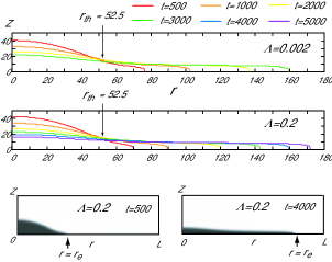
Figure 1: (Color online) Shapes of an axisymmetric droplet spreading on a cooler substrate with $T_{w}=0.870T_{c}$ at various times for $\Lambda=0.002$ (top) and $0.2$ (middle) in the $r$-$z$ plane. The system temperature was initially $T_{0}=0.875T_{c}$ at $t=0$. The boundary position between the main body of the droplet and the precursor film is fixed at $r=r_{{\rm th}}=52.5\ell$ for both $\Lambda$. The edge position $r_{e}(t)$ of the film increases with time as illustrated in the bottom plates.

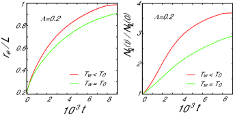
Figure 2: (Color online) Time evolutions of the edge position $r_{e}(t)$ divided by $L$ (left) and the particle number in the droplet $N_{\ell}(t)$ divided by $N_{\ell}(0)$ (right) for $\Lambda=0.2$. Two curves correspond to $T_{w}=0.870T_{c}<T_{0}$ (red) and $T_{w}=0.875T_{c}=T_{0}$ (green). The interface curve is determined by Eq.(4.2). The film edge reaches the side wall at $t\sim 10^{4}$. Condensation occurs faster in the cooled case than in the non-cooled case.

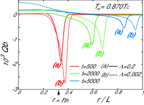
Figure 3: (Color online) Heat flux on the substrate $Q_{\rm b}(r,t)$ as a function of $r$ in units of $\epsilon\ell/v_{0}\tau_{0}$ at various times for $T_{w}=0.870T_{c}<T_{0}$ with $\Lambda=0.002$ and $0.2$. A negative peak at the film edge indicates absorption of latent heat from the fluid to the solid. At long times this absorption becomes weaker and there appears a heat flow from the solid to the fluid for $r<r_{\rm th}$.

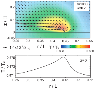
Figure 4: (Color online) Temperature $T$ around an advancing film edge at $t=1000$, where $T_{w}=0.870T_{c}$ and $\Lambda=0.2$. In the top, the color represents the temperature according to the color map, and the velocity field is shown by arrows with its maximum being $1.4\times 10^{-2}\ell/\tau_{0}$ as indicated below the plate. In the bottom, the substrate temperature at $z=0$ is plotted, which is maximum at the edge position due to a finite thermal conductivity of the solid.

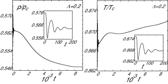
Figure 5: Pressure (left) and temperature (right) vs $t$ at the point $(z/H,r/L)=(0.48,0.5)$ far from the substrate in gas, where $T_{w}=0.870T_{c}$ and $\Lambda=0.2$. Their short time behavior ($t<200$) is due to propagation of a low-pressure sound pulse and is adiabatic (inset), while their long time behavior is due to gradual condensation.

IV.1 Evolution on long and short time scales

In Fig.1, the droplet spreads over the substrate in the complete wetting condition for $\Lambda=0.002$ and 0.2. The liquid region is divided into the droplet body in the region $r<r_{\rm th}$ and the precursor film in the region $r_{\rm th}<r<r_{e}(t)$. In our simulation, $r_{\rm th}$ is equal to $52.5\ell=0.26L$ independently of time, while $r_{e}(t)$ increased in time. The film thickness $\ell_{f}$ was only weakly dependent on time being about $5\ell$ for both $\Lambda$ (see the film profiles in Fig.6 below). However, for slightly deeper cooling (say, for $T_{w}=0.868T_{c}$) or for slightly larger $\Phi_{1}$ (say, for $\Phi_{1}=0.065$), a new liquid region (a ring here) appeared on the substrate ahead of the precursor film.

In Fig.2, we show $r_{e}(t)$ and the particle number in the liquid region $N_{\ell}(t)$ vs $t$ for $\Lambda=0.2$ in the cooled case with $T_{w}=0.870T_{c}$ and the non-cooled case with $T_{w}=T_{0}=0.875T_{c}$. We calculate $N_{\ell}(t)$ from

$$N_{\ell}(t)=2\pi\int_{0}^{r_{e}(t)}drr\int_{0}^{z_{\rm int}(r,t)}dz~{}n({\mbox{\boldmath$r$}},t),$$ (4.1)

where the interface height is at $z=z_{\rm int}(r,t)$ in the range $0<r<r_{e}(t)$. It starts from the initial number $N_{\ell}(0)=0.67\times 10^{5}\ell^{3}/v_{0}$ and becomes a few times larger at $t\sim 10^{4}$. Here condensation takes place even for the non-cooled case with $T_{w}=T_{0}$. In these two cases, the latent heat due to condensation is mostly absorbed by the solid reservoir. In calculating $N_{\ell}(t)$ we determine the film height $z_{\rm int}(r,t)$ from the relation,

$$n(r,z_{\rm int},t)=(n_{\ell}^{0}+n_{g}^{0})/2,$$ (4.2)

where $n_{\ell}^{0}=0.579v_{0}^{-1}$ and $n_{g}^{0}=0.123v_{0}^{-1}$ are the densities on the coexistence curve at $T=0.875T_{c}$. In our case, the film is so thin and there is no unique definition of $z_{\rm int}$.

In Fig.3, we display the heat flux on the substrate $Q_{\rm b}(r,t)$ for the same runs. From Eq.(3.7) it is defined in terms of the temperature gradient $T^{\prime}=\partial T/\partial z$ as

$$Q_{\rm b}(r,t)=-(\lambda_{w}T^{\prime})_{z=-0}=-(\lambda T^{\prime})_{z=+0}.$$ (4.3)

Negative peaks indicate absorption of latent heat from the fluid to the substrate around the film edge. However, at long times ($t=5000$ in the figure) heat is from the solid to the fluid in the region of the droplet body $r<r_{\rm th}$. The amplitude of $Q_{\rm b}(r,t)$ around the peak is larger for $\Lambda=0.002$ than for $\Lambda=0.2$, obviously because heat is more quickly transported for smaller $\Lambda$ or for larger $\lambda_{w}$. Also $Q_{\rm b}(r,t)$ is sensitive to $T_{0}-T_{w}$. For example, in the non-cooled case $T_{w}=T_{0}$, the minima of $Q_{\rm b}(r,t)$ became about half of those in Fig.3 (not shown here). In our previous simulation Teshi , a positive peak of $Q_{\rm b}(r,t)$ was found at the contact line of an evaporating droplet.

In the upper panel of Fig.4, we show the temperature near the edge at $t=1000$, where $\Lambda=0.2$ and $T_{w}=0.870T_{c}<T_{0}$. It exhibits a hot spot in the gas side produced by latent heat. In this run, the peak height of the hot spot $T_{\rm p}$ depended on $t$ as $10^{-2}(T_{\rm p}-T_{w})/T_{c}=1.0$, $0.7$,$0.5$, and $0.4$ for $10^{-3}t=1,2,3$, and $4$. The maximum of the gas velocity $v_{g}$ is $0.014$ around the hot spot, while the edge speed is a few times faster as $dr_{e}/dt\sim 0.04$. The corresponding Reynolds number $v_{g}\ell_{f}/\nu_{0}$ in the gas is very small $(\sim 0.07$ here). In the non-cooling case $T_{w}=T_{0}$ the peak height was reduced to $T_{\rm p}-T_{0}=0.007T_{c}$ and $v_{g}$ to $0.008$ at $t=10^{3}$. In the lower panel of Fig.4, the substrate temperature at $z=0$ is maximum at the film edge. Such a temperature variation in the solid should be measurable Stephan .

In Fig.5, we display the time evolution of the pressure and the temperature at the position $(z,r)=(0.48H,0.5L)$ in the gas region far from the substrate in the case $T_{w}=0.870T_{c}$ and $\Lambda=0.2$. In the inset, their initial deviations originate from a lower-pressure sound pulse emitted from the adsorption layer in Eq.(3.9). This acoustic process is an example of the piston effect Ferrell ; Miura . In this case the thermal diffusion layer due to cooling of the substrate gives rise to a smaller effect. The emitted pulse traverses the cell on the acoustic time $H/c_{g}\sim 50$ and is reflected at the top plate, where $c_{g}\sim 4$ is the sound velocity in the gas. The deep minimum of $T$ below $T_{w}$ and that of $p$ at $t\sim 25$ are due to its first passage. Here the adiabatic relation $\delta T=(\partial T/\partial p)_{s}\delta p$ is well satisfied for the deviations $\delta T=T-T_{0}$ and $\delta p=p-p_{0}$. The adiabatic coefficient $(\partial T/\partial p)_{s}$ is equal to $11T_{c}/p_{c}$ in the gas and is larger than that in the liquid by one order of magnitude. On long time scales, Fig.5 shows that the pressure gradually decreases with progress of condensation, while the temperature increases for $200\lesssim t\lesssim 1500$, slowly decreases for $1500\lesssim t\lesssim 3000$, and again increases for longer $t$. The gas temperature in the middle region is slightly higher than $T_{w}$ by $0.002T_{c}$ at $t=9000$. We note that the gas temperature is influenced by a gas flow from the droplet and behaves in a complicated manner.

IV.2 Profiles of density, temperature, and pressure

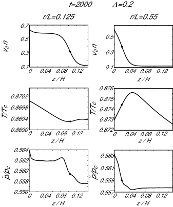
Figure 6: Density (top), temperature (middle), and normal pressure (bottom) as functions of the distance $z$ from the substrate at $r/L=0.125$ (left) and at $r/L=0.55$ (right), where $t=2000$, $T_{w}=0.870T_{c}$, and $\Lambda=0.2$. The former path passes through the droplet body, while the latter through the film edge. The black dot $\bullet$ on each curve indicates the interface position determined by Eq.(4.2).

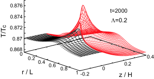
Figure 7: (Color online) Temperature $T$ around a film edge in the fluid (red) and in the solid (black) in the $r$-$z$ plane at $t=2000$, where $T_{w}=0.870T_{c}$ and $\Lambda=0.2$. See Fig.4 for the hot spot at $t=1000$ in color in the same run.

In Fig.6, we show the profiles of the density $n$, the temperature $T$, and the the stress component $\tilde{p}$ along the density gradient at $t=2000$ for $\Lambda=0.2$ and $T_{w}=0.870T_{c}$. We define $\tilde{p}$ as

$${\tilde{p}}=\sum_{ij}\hat{\nu}_{i}\hat{\nu}_{j}\Pi_{ij}=p-CT(n\nabla^{2}n-|\nabla n|^{2}/2),$$ (4.4)

where $\Pi_{ij}$ is the reversible stress tensor in Eq.(2.11), $p$ is the van der Waals pressure, and $\hat{\mbox{\boldmath$\nu$}}=\{\hat{\nu}_{i}\}=\{\nabla_{i}n/|\nabla n|\}$ is the unit vector along the density gradient $\nabla n$. Thus $\tilde{p}$ is called the normal pressure. Obviously, ${\tilde{p}}\cong p$ in the bulk region. In equilibrium, $\tilde{p}$ is equal to the saturation pressure $p_{\rm cx}(T)$ for a planar interface OnukiV , while it changes by the Laplace pressure difference $2\gamma/R$ along $\hat{\mbox{\boldmath$\nu$}}$ across an interface with mean curvature $1/R$. In nonequilibrium, we find that inhomogeneity of $\tilde{p}$ around an interface is much weaker than that of $p$ itself. The left panels for $r=0.125L<r_{\rm th}$ in Fig.6 indicate weak adsorption near the wall in Eq.(3.9), a well-defined interface at $z\sim 20$, and a negative temperature gradient within the droplet body. For this $r$, a heat flow is from the solid to the fluid. In the right panels for $r=0.55L>r_{\rm th}$ in Fig.6, $n$ decreases from a liquid density near the wall to a gas density without a region of a flat density and $T$ exhibits a peak at the hot spot. Furthermore, Fig.7 gives a bird view of the temperature near the edge from the same run, which corresponds to the middle right panel in Fig.6. Here the temperature inhomogeneity in the solid can also be seen.

It is of interest how the normal pressure and the temperature ($\tilde{p}$,$T$) at the interface is close to the coexistence line ($p_{\rm cx}(T),T)$ in the $p$-$T$ phase diagram. We define

$$h=\frac{T-T_{0}}{T_{c}}-{\bigg{(}}\frac{\partial{T}}{\partial{p}}{\bigg{)}}_{\rm cx}\frac{{\tilde{p}}-p_{0}}{T_{c}},$$ (4.5)

where the derivative $({\partial T}/{\partial p})_{\rm cx}$ along the coexistence line is equal to $0.38T_{c}/p_{c}$ at $T=0.875T_{c}$. The upper panel of Fig.8 displays $h$ around the film at $t=1000$, while the lower panel of Fig.8 gives $h$ along the surface $z=z_{\rm int}$ at four times for $\Lambda=0.2$ and 0.002. This quantity represents the distance from the coexistence line $p=p_{\rm cx}(T)$. In the bulk region, $h<0$ in stable liquid and metastable gas, while $h>0$ in stable gas and metastable liquid. We can see that $h$ nearly vanishes in the droplet body $r<r_{\rm th}$ and increases in the film $r_{\rm th}<r<r_{e}(t)$, but $h$ remains less than $10^{-2}$ even at the edge. Note that the Laplace pressure contribution to $h$ is $({\partial T}/{\partial p})_{\rm cx}2\gamma/T_{c}R$, which is of order $0.01$ in the droplet body $r<r_{\rm th}$ at $t=1000$.

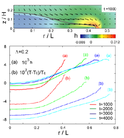
Figure 8: (Color online) Top: Distance from the coexistence line $h$ in Eq.(4.5) at $t=1000$ in color, which is negative in the droplet body and is positive in the film and in the gas. Here $T_{w}=0.870T_{c}$ and $\Lambda=0.2$. Bottom: (a) $h$ and (b) $(T-T_{0})/T_{c}$ along the interface at four times. For $r<r_{\rm th}$, $|h|$ is smaller than $(T_{0}-T)/T_{c}$. For $r>r_{\rm th}$, the distance from the coexistence line increases.

IV.3 Condensation rate and gas velocity

In our previous simulationTeshi , evaporation of a thick liquid droplet mostly takes place in the vicinity of the contact line in the partial wetting condition. We here examine the space dependence of the condensation rate of a thin fim in the complete wetting condition.

We introduce the number flux $J(r,t)$ from gas to liquid along $\hat{\mbox{\boldmath$\nu$}}=|\nabla n|^{-1}\nabla n$ through the interface,

$$J(r,t)=n({\mbox{\boldmath$v$}}-{\mbox{\boldmath$v$}}_{int})\cdot{\hat{\mbox{\boldmath$\nu$}}},$$ (4.6)

where ${\mbox{\boldmath$v$}}_{int}$ is the interface velocity. If $J$ is regarded as a function of the coordinate along the normal direction $\hat{\mbox{\boldmath$\nu$}}$, it is continuous through the interface from the number conservation, while $n$ and ${\mbox{\boldmath$v$}}\cdot\hat{\mbox{\boldmath$\nu$}}$ change discontinuously. Thus we may well determine $J$ on the interface. If it is positive, it represents the local condensation rate per unit area. In Fig.9, we plot $J(r,t)$ vs $r/L$ in the region $0<r<r_{e}(t)$ at three times for $\Lambda=0.002$ and 0.2 in the cooled case $T_{w}=0.870T_{c}$. We recognize that $J(r,t)$ steeply increases in the precursor film and is maximum at the edge. Moreover, it becomes negative in the body part $r<r_{\rm th}$ at $t=3000$, where evaporation occurs.

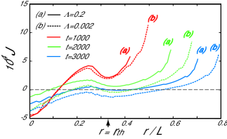
Figure 9: (Color online) Flux $J(r,t)$ on the interface in units of $\ell/v_{0}\tau_{0}$ vs $r/L$ in the region $0<r<r_{e}(t)$ at $10^{-3}t=1$, $2$, and $3$ for $T_{w}=0.870T_{c}$ in the two cases of $\Lambda=0.002$ and 0.2. A precursor film is on the left of the arrow (see Fig.1). In its positive region it is the condensation rate. In its negative region evaporation takes place.

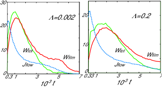
Figure 10: (Color online) Total condensation rate $W_{\rm tot}(t)$ (green), condensation rate onto the film $W_{\rm film}(t)$ (red), and flow from the droplet body to the film $J_{\rm flow}(t)$ (blue) in units of $\ell^{3}/v_{0}\tau_{0}$ as functions of time. The time range is $[3\times 10^{2},7\times 10^{3}]$ for $\Lambda=0.002$ (left) and $[3.3\times 10^{2},7\times 10^{3}]$ for $\Lambda=0.2$ (right).

The total condensation rate $W_{\rm tot}(t)$ is the surface integral of $J(r,t)$ on all the surface. The surface area in the range $[r,r+dr]$ is $da=2\pi drr/\sin\theta$, where $\theta$ is the angle between $\hat{\mbox{\boldmath$\nu$}}$ and the $r$ axis. Thus,

$$W_{\rm tot}(t)=2\pi\int_{0}^{r_{\rm c}}dr~{}{r}J(r,t)/{\sin\theta}.$$ (4.7)

The particle number in the liquid region $N_{\ell}(t)$ in Eq.(4.1) increases in time as

$$\frac{d}{dt}N_{\ell}(t)=W_{\rm tot}(t).$$ (4.8)

We also define the condensation rate in the film region,

$$W_{\rm film}(t)=2\pi\int_{r_{\rm th}}^{r_{e}(t)}dr~{}{r}J(r,t)/{\sin\theta},$$ (4.9)

where $\sin\theta\cong 1$. In this integral the vicinity of the edge gives rise to a main contribution. In fact, the contribution from the region $r_{e}-16\ell<r<r_{e}$ is about $50\%$ of the total contribution from the region $r_{\rm th}<r<r_{e}$. Therefore, in terms of the gas velocity $v_{g}$ and the gas density $n_{g}$ around the edge, we estimate $W_{\rm film}(t)$ as

$$W_{\rm film}(t)\sim 2\pi r_{e}{n}_{g}v_{g}\ell_{c},$$ (4.10)

where $\ell_{c}$ is the width of the condensation area estimated to be about $30\ell$.

The flux from the droplet body to the film is given by

$$J_{\rm flow}(t)=2\pi r_{\rm th}\int_{0}^{z_{\rm th}}dz~{}n(r_{\rm th},z,t)v_{r}(r_{\rm th},z,t),$$ (4.11)

where $v_{r}(r,z,t)=v_{x}x/r+v_{y}y/r$ is the velocity in the plane within the film. This lateral flux is defined at $r=r_{\rm th}$. More generally, we may introduce the flux

$$J_{\rm f}(r,t)=2\pi r\int_{0}^{z_{\rm th}}dz~{}n(r,z,t)v_{r}(r,z,t),$$ (4.12)

for $r\geq r_{\rm th}$ with $z_{\rm th}$ being the film thickness $\ell_{f}$. Then $J_{\rm flow}(t)=J_{\rm f}(r_{\rm th},t)$. In the presence of condensation onto the film, $J_{\rm f}(r,t)$ increases with increasing $r$. Its maximum $J_{\rm f}(r_{e}(t),t)$ is estimated as $2\pi r_{e}{\bar{n}}_{\ell}v_{\ell}\ell_{f}$, where ${\bar{n}}_{\ell}$ is the average density in the film and $v_{\ell}$ is the average fluid velocity in the film. At $t=1000$ (or $4000)$, the ratio $J_{\rm f}(r_{e}(t),t)/J_{\rm f}(r_{\rm th},t)$ was equal to 1.1 (or 2.4) for $\Lambda=0.2$.

In terms of $W_{\rm film}(t)$ and $J_{\rm flow}(t)$, the particle number in the film, written as $N_{\rm film}(t)$, changes in time as

$$\frac{d}{dt}N_{\rm film}(t)=W_{\rm film}(t)+J_{\rm flow}(t).$$ (4.13)

Using the edge velocity $\dot{r}_{e}=d{r}_{e}/dt$, we also obtain

$$\frac{d}{dt}N_{\rm film}(t)=2\pi r_{e}\dot{r}_{e}{\bar{n}}_{\ell}\ell_{f},$$ (4.14)

since the film thickness is fixed in our case. In Fig.10, we plot $W_{\rm tot}(t)$, $W_{\rm film}(t)$, and $J_{\rm flow}(t)$ vs $t$ for $\Lambda=0.002$ and 0.2. In an early stage ($t<1.5\times 10^{3}$ for $\Lambda=0.002$ and $t<2.6\times 10^{3}$ for $\Lambda=0.2$), $W_{\rm tot}(t)$ is larger than $W_{\rm film}(t)$, where condensation occurs on all the interfaces. Afterwards, the reverse relation $W_{\rm tot}(t)<W_{\rm film}(t)$ holds, where evaporation occurs in the droplet body $r<r_{\rm th}$. We also notice $W_{\rm film}(t)>J_{\rm flow}(t)$ for $t\gtrsim 1000$ for these two $\Lambda$. This means that the film extends mainly due to condensation near the film edge except in the early stage. For example, at $t=1000$ (or $4000$), we have the edge velocity ${\dot{r}}_{e}=0.04$ (or $0.012$) and the gas velocity $v_{g}=0.012$ (or $0.0064$) near the edge in the case $\Lambda=0.2$. The fluid velocity ${\bar{v}}_{\ell}$ in the film is $0.015$ (or $0.005$) at $r=r_{\rm th}$. These values surely yield $W_{\rm film}(t)\sim J_{\rm flow}(t)$ at $t=1000$ and $W_{\rm film}(t)\sim 3J_{\rm flow}(t)$ at $t=4000$ in accord with their curves in the right panel of Fig.10 and are consistent with Eqs.(4.13) and (4.14). Thus, condensation near the film edge can be the dominant mechanism of the precursor film growth, as originally expected by Hardy Hardy ; PG .

We next estimate the gas velocity $v_{g}$ near the edge. The heat flux is of order $\lambda_{\ell}(T_{\rm p}-T_{w})/\ell_{f}$ there, where $T_{\rm p}$ is the peak temperature and $\lambda_{\ell}$ is the liquid thermal conductivity. It balances with the convective latent heat flux $\sim n_{g}T_{0}\Delta sv_{g}$ in the gas, where $n_{g}$ is the gas density and $\Delta s$ is the entropy difference per particle. Therefore,

$$v_{g} \sim\lambda_{\ell}(T_{\rm p}-T_{w})/(\ell_{f}n_{g}T_{0}\Delta s)$$ (4.15)

$$\sim(T_{\rm p}-T_{w}){\bar{n}}_{\ell}\nu_{0}/(T_{0}n_{g}\ell_{f}),$$

where we set $\lambda_{\ell}=k_{B}\nu_{0}{\bar{n}}_{\ell}$ and $\Delta s(=2.1k_{B}$ here) in the second line. For example, in the upper plate of Fig.4 at $t=1000$ we have $v_{g}=0.014$, while the second line of Eq.(4.15) gives 0.012 with $\ell_{f}/\ell\sim 5$ and ${\bar{n}}_{\ell}/n_{g}\sim 5$.

V Spreading and Evaporation on a heated substrate

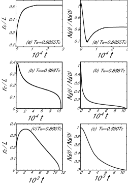
Figure 11: Time evolutions of the edge position $r_{e}(t)$ divided by $L$ (left) and the particle number in the droplet $N_{\ell}(t)$ divided by $N_{\ell}(0)$ (right) for $\Lambda=0.2$. The temperature $T_{w}$ at the solid bottom was raised at $t=0$ from $0.875T_{c}$ to (a) $0.8855T_{c}$ (top), (b) $0.888T_{c}$ (middle), and (c) $0.890T_{c}$ (bottom). The fluid tends to a steady two-phase state in (a), where the liquid region assumes a pancake thin film. The liquid evaporates to vanish on a time scale of $10^{5}$ in (b) and $10^{4}$ in (c).

Next, we present simulation results of a heated liquid droplet in the complete wetting condition, where $T_{w}$ is increased above $T_{0}=0.875T_{c}$ at $t=0$ with $\Lambda=0.2$. The other parameter values are the same as those in the previous section. The preparation method of a droplet is unchanged. Then a precursor film develops in an early stage (at least for small $T_{w}-T_{0}$), because of the complete wetting condition at $\Phi_{1}=0.061$ (see Eq.(3.4)). A new aspect is that evaporation dominates over condensation with increasing $T_{w}-T_{0}>0$. The experiment by Gu$\acute{\rm e}$na et al.Caza corresponds to this situation (see Section 1).

In Fig.11, we show the edge position $r_{e}(t)$ and the particle number in the liquid $N_{\ell}(t)$ as functions of $t$ for three cases (a) $T_{w}=0.8855T_{c}$, (b) $0.888T_{c}$, and (c) $0.890T_{c}$. In the weakest heating case (a) with $T_{w}-T_{0}=0.0105T_{c}$, $r_{e}(t)$ and $N_{\ell}(t)$ tend to constants at long times, where a thin pancake-like film is realized with radius $\sim 0.5L$ and thickness $\sim 4\ell$ in a steady state. For higher $T_{w}$, evaporation dominates over condensation and the liquid region eventually disappears. Thus, if $T_{w}-T_{0}$ exceeds a critical value, a liquid droplet has a finite lifetime due to evaporation even in the complete wetting condition. From Fig.11, this lifetime is of order $10^{5}$ at $T_{w}-T_{0}=0.018T_{c}$ in (b) and $10^{4}$ at $T_{w}-T_{0}=0.020T_{c}$ in (c).

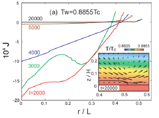
Figure 12: (Color online) Mass flux $J(r,t)$ through the interface in Eq.(4.6) for the weakly heated case $T_{w}=0.8855T_{c}$ corresponding to (a) in Fig.11. Evaporation takes place in the region $J<0$ except close to the edge. Here $J$ decreases in time. A steady two-phase state is approached at long times, where $J$ is nonvanishing only near the edge. Inset: temperature in color and velocity represented by arrows at $t=20000$.

Figure 13: (Color online) Mass flux through the interface $J(r,t)$ in Eq.(4.6) for the highest heating case $T_{w}=0.890T_{c}$ corresponding to (c) in Fig.11. Here evaporation takes place over the whole surface and the liquid disappears at $t=11000$. The inset displays the fim shape at $t=3000$, where $N_{\ell}(t)$ is half of the initial value.

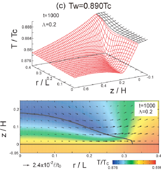
Figure 14: (Color online) Top: Temperature $T$ in the region $0<r/L<0.4$ and $-0.1<z/H<0.7$ at $t=1000$ in the highest heating $T_{w}=0.890T_{c}$ corresponding to (c) in Fig.11. Bottom: temperature in color and velocity by arrows at the same time in the same run. A liquid film supports a large temperature gradient and evaporation occurs all over the surface, while the temperature above the film is nearly flat due to a gas flow.

In Fig.12, we show the mass flux through the interface $J(r,t)$ defined in Eq.(4.6) in the weakly heated case (a) $T_{w}=0.8855T_{c}$. Its negativity implies evaporation. In the region far from the edge, evaporation is marked in transient states ($t\lesssim 4000$), but it tends to vanish at long times. We can also see the region of positive $J$ with width of order 10 near the edge ($r_{e}-10<r<r_{e}$), where the film is still flat and the angle $\theta$ in Eq.(4.7) is nearly $\pi/2$. In Fig.12, however, we do not show $J$ just at the edge ($r\cong r_{e}(t)$ and $0<z<\ell_{f}$), where $\theta$ changes from $\pi/2$ to zero in the $z$ direction and evaporation occurs ($J<0$). As a balance of condensation and evaporation in these two regions, the total condensation rate $W_{\rm tot}$ in Eq.(4.7) tends to vanish at long times, while there is no velocity field in the region $r<r_{e}-10$. In the inset of Fig.12, the velocity field around the edge is displayed at $t=20000$, where the maximum gas velocity is $v_{g}=1.1\times 10^{-3}\ell/\tau_{0}$.

In Fig.13, we show $J(r,t)$ at several times in the highest heating case (c) $T_{w}=0.890T_{c}$. In the whole surface, $J$ is negative and evaporation ocuurs. For $t\lesssim 40000$ evaporation is strongest at the fim center. At long times ($t=8000$ here), it becomes weakest at the film center. Figure 14 is produced by the same run. It gives a bird view of the temperature and a snapshot of the velocity field in the vicinity of the film edge at $t=1000$. We can see a steep temperature gradient within the film, which is much larger than in the gas, leading to a strong heat flux from the solid to the film. In this manner, evaporation is induced all over the surface and is strongest at the film center in the early stage. It is remarkable that the temperature gradient nearly vanishes in the gas region above the film away from the edge, where heat is transported by a gas flow. We can also see a significant temperature inhomogeneity in the solid part in contact with the film.

VI Summary and remarks

For one-component fluids we have examined spreading of a small droplet on a smooth substrate in the complete wetting condition in the axisymmetric geometry. In the dynamic van der Waals theory OnukiPRL ; OnukiV , we have integrated the entropy equation in Eq.(2.14) together with the continuity and momentum equations. This method may remove artificial flows around an interface para . In our phase field scheme, we need not introduce any surface boundary conditions. The condensation rate on the interface is a result and not a prerequisite of the calculation. We have also assumed that the substrate wall has a finite thickness $H_{w}$ and the solid temperature obeys the thermal diffusion equation, whereas an isothermal substrate is usually assumed in the literature. The temperature $T_{w}$ at the solid bottom $z=-H_{w}$ is a new control parameter in our simulation. Cooling (Heating) the fluid is realized by setting $T_{w}$ lower (higher) than the initial fluid temperature $T_{0}$. We give salient results in our simulation.

(i) In the cooled and non-cooled cases with $T_{w}\leq T_{0}$, a precursor film with a constant thickness has appeared ahead of the droplet body. Here the liquid volume has increased in time due to condensation on the film surface. In an very early stage, the piston effect comes into play due to sound propagation Ferrell ; Miura . At long times, the condensation rate has become localized near the film edge and the film has expanded dominantly due to condensation. As a result, a hot spot has appeared near the film edge due to the latent heat released.

(ii) At a critical value of $T_{w}$ slightly higher than $T_{0}$, we have realized a steady-state thin liquid film, where condensation and evaporation are localized and balanced at the edge. For higher $T_{w}$, evaporation has dominated and the liquid region has disappeared eventually. This lifetime decreases with increasing $T_{w}-T_{0}$. For a thin film, evaporation has appeared all over the film surface upon heating. In our previous simulation for one-component fluids Teshi evaporation of a thick droplet was mostly localized near the contact line in the partial wetting condition.

We give some critical remarks. (1) If the mesh length $\Delta x=\ell/2$ is a few $\rm\AA$, our system length is on the order of several ten manometers and the particle number treated is of order $10^{6}$ (see Sec.IIIC). Our continuum description should be imprecise on the angstrom scale. Thus examination of our results by large-scale molecular dynamics simulations should be informative. We should also investigate how our numerical results can be used or modified for much larger droplet sizes. (2) In future work, we shoud examine the role of the long-range van der Waals interaction in the wetting dynamics. As is well-known, it crucially influences the film thickness PG . (3) We should also include the slip effect at the contact line in our scheme slip ; Qian . (4) We should study the two-phase hydrodynamics in fluid mixtures, where a Marangoni flow decisively governs the dynamics even at small solute concentrations Str ; Larson ; maran .

- (1) P.G. de Gennes, Rev. Mod. Phys. 57, 827 (1985).
- (2) W. Hardy, Philos.Mag. 38, 49 (1919). See Ref.PG for comments on this original work.
- (3) V.E. Dussan, Ann. Rev. Fluid Mech. 11, 371 (1979).
- (4) L. Leger and J. F. Joanny, Rep. Prog. Phys. 55, 431 (992).
- (5) D. Bonn, J. Eggers, J. Indekeu, J. Meunier, and E. Rolley, Rev. Mod. Phys. 81, 740 (2009).
- (6) D. Ausserr, A. M. Picard, and L. Lger Phys. Rev. Lett. 57, 2671 (1986).
- (7) F. Heslot, A. M. Cazabat, and P. Levinson Phys. Rev. Lett. 62, 1286 (1989); F. Heslot, A. M. Cazabat, P. Levinson, and N. Fraysse ibid. 65, 599 (1990).
- (8) J.-X. Yang, J. Koplik, and J. R. Banavar, Phys. Rev. A 46, 7738 (1992).
- (9) J. A. Nieminen, D. B. Abraham, M. Karttunen, and K. Kaski, Phys. Rev. Lett. 69, 124 (1992).
- (10) T. Ala-Nissila, S. Herminghaus, T. Hjelt, and P. Leiderer, Phys. Rev. Lett. 76, 4003 (1996); T. Hjelt, S. Herminghaus, T. Ala-Nissila, and S. C. Ying, Phys. Rev. E 57, 1864 (1998).
- (11) J. A. Nieminen and T. Ala-Nissila, Phys. Rev. E 49, 4228 (1994); M. Haataja, J. A. Nieminen, and T. Ala-Nissila, ibid. 52, R2165 (1995);
- (12) J. De Coninck, U. d fOrtona, J. Koplik, and J. R. Banavar, Phys. Rev. Lett. 74, 928 (1995); U. d fOrtona, J. De Coninck, J. Koplik, and J. R. Banavar, Phys. Rev. E 53, 562 (1996).
- (13) J. Koplik, S. Pal, and J.R. Banavar, Phys. Rev. E 65, 021504 (2002).
- (14) A. Milchev and K. Binder, J. Chem. Phys. 116, 7691 (2002).
- (15) E. B. Webb III, G. S. Grest and D. R. Heine, Phys. Rev. Lett. 91, 236102 (2003).
- (16) G. Guna, C. Poulard, and A.M. Cazabat, Colloid and Interface Science 312 (2007) 164.
- (17) J. Hegseth, A. Oprisan, Y. Garrabos, V. S. Nikolayev, C. Lecoutre-Chabot, and D. Beysens Phys. Rev. E 72, 031602 (2005).
- (18) R.D. Deegan, O. Bakajin, T.F. Dupont, G. Huber, S.R. Nagel, and T.A. Witten, Nature 389, 827 (1997).
- (19) H. Hu and R.G. Larson, Langmuir 21, 3972 (2005).
- (20) N. Shahidzadeh-Bonn, S. Rafai, A. Azouni, and D. Bonn, J. Fluid. Mech. 549, 307 (2006).
- (21) H. J. Butt, D. S. Glovko, and E. Bonaccurso, J. Phys. Chem B 111, 5277 (2007).
- (22) R. Teshigawara and A. Onuki, Europhys. Lett. 84, 36003 (2008).
- (23) J. Straub, Int. J. Therm. Sci. 39, 490 (2000).
- (24) V.S. Nikolayev, D.A. Beysens, G.-L. Lagier, and J. Hegseth, Int. J. of Heat and Mass Transfer 44, 3499 (2001).
- (25) C. Hhmann, P. Stephan Experimental Thermal and Fluid Science 26, 157 (2002). In this boiling experiment, the substrate temperature exhibited a sharp drop by K near a contact line in a narrow region of m length.
- (26) D. Beysens, Y. Garrabos, V. S. Nikolayev, C. Lecoutre-Chabot, J.-P. Delville, and J. Hegseth, Europhys. Lett. 59, 245 (2002).
- (27) A. Onuki and K. Kanatani, Phys. Rev. E 72, 066304 (2005).
- (28) A. Onuki, Phys. Rev. E 79, 046311 (2009).
- (29) P. Ehrhard and S. H. Davis, J. Fluid Mech. 229, 365 (1991); D. M. Anderson and S.H. Davis, Phys. Fluids, 7, 248 (1995).
- (30) P. Seppecher, Int. J. Engng Sci. 34, 977 (1996).
- (31) D. Jasnow and J. Vials, Phys. Fluids 8, 660 (1996). R. Chella and J. Vials, Phys. Rev E 53, 3832 (1996).
- (32) D.M. Anderson, G.B. McFadden, and A.A. Wheeler, Annu. Rev. Fluid Mech. 30, 139 (1998).
- (33) D. Jacqmin, J. Comput. Phys. 155, 96 (1999).
- (34) D. Jamet, O. Lebaigue, N. Coutris and J. M. Delhaye, J. Comput. Phys. 169, 624 (2001).
- (35) R. Borcia and M. Bestehorn, Phys. Rev. E 67, 066307 (2003); ibid. 75, 056309 (2007).
- (36) T. Araki and H. Tanaka, Europhys. Lett. 65, 214 (2004).
- (37) B. J. Palmer and D. R. Rector, Phys. Rev. E 61, 5295 (2000). In an erratum to this paper (ibid. 69, 049903(E) (2004)), they pointed out a difficulty of the lattice Boltzmann algorithm in simulations of evaporation.
- (38) A. J. Briant, A.J. Wagner, and J. M. Yeomans, Phys. Rev. E 69, 031602 (2004).
- (39) T. Inamuro, T. Ogata, S. Tajima, N. Konishi, J. Comput. Phys. 198, 628 (2004).
- (40) C.M. Pooley, O. Kuksenok, and A.C. Balazs, Phys. Rev. E 71, 030501 (R) (2005).
- (41) A. Onuki, Phys. Rev. Lett. 94, 054501 (2005).
- (42) A. Onuki, Phys. Rev. E 75, 036304 (2007). In this paper, the energy equation (2.13) was integrated, resulting in a parasitic flow around an interface in Figs.3 and 6.
- (43) N. Takada and A. Tomiyama, Inter. J. of Mod, Phys. C 18, 5360 (2007).
- (44) G. Gonnella, A Lamura, and A Piscitelli, J. Phys. A: Math. Theor. 41, 105001 (2008).
- (45) A. Kawasaki, J. Onishi, Y. Chen, and H. Ohashi, Computers Mathematics with Applications 55, 1492 (2008).
- (46) G. Fang and C. A. Ward, Phys. Rev. E, 59, 417 (1999).
- (47) A. Onuki, Phase Transition Dynamics (Cambridge University Press, Cambridge, 2002).
- (48) L.D. Landau and E.M. Lifshitz, Fluid Mechanics (Pergamon, 1959).
- (49) If we set not including the potential , the term appears in the right hand side of Eq. (2.13) OnukiV .
- (50) J. Koplik, J.R. Banavar, and J.F. Willemsen, Phys. Rev. Lett. 60, 1282 (1988); P.A. Thompson and M.O. Robbins, ibid. 63, 766 (1989); J. L. Barrat and L. Bocquet, ibid. 82, 4671 (1999).
- (51) T. Qian, X. -P. Wang, and P. Sheng, Phys. Rev. E 68, 016306 (2003).
- (52) B. Lafaurie, C. Nardone, R. Scardovelli, S. Zaleski, and G. Zanetti, J. Comput. Phys. 113, 134 (1994); I. Ginzburg and G. Wittum, J. Comput. Phys. 166, 302 (2001); D. Jamet, D. Torres, and J. U. Brackbill, J. Comput. Phys. 182, 262 (2002); S. Shin, S. I. Abdel-Khalik, V. Daru, and D. Juric, J. Comput. Phys. 203, 493 (2005).
- (53) A. Onuki and R.A. Ferrell, Physica A 164, 245 (1990); A. Onuki, Phys. Rev. E 76, 061126 (2007).
- (54) Y. Miura, S. Yoshihara, M. Ohnishi, K. Honda, M. Matsumoto, J. Kawai, M. Ishikawa, H. Kobayashi, and A. Onuki, Phys. Rev. E 74, 010101 (R) (2006).