The potential of Red Supergiants as extra-galactic abundance probes at low spectral resolution

Abstract

Red Supergiants (RSGs) are among the brightest stars in the local universe, making them ideal candidates with which to probe the properties of their host galaxies. However, current quantitative spectroscopic techniques require spectral resolutions of R$\mathrel{\hbox{\hbox to0.0pt{\hbox{\lower 4.0pt\hbox{$\sim$}}\hss}\hbox{$>$}}}$17,000, making observations of RSGs at distances greater than 1Mpc unfeasible. Here we explore the potential of quantitative spectroscopic techniques at much lower resolutions, $R\approx$2-3000. We take archival $J$-band spectra of a sample of RSGs in the Solar neighbourhood. In this spectral region the metallic lines of Fe i, Mg i, Si i and Ti i are prominent, while the molecular absorption features of OH, H₂O, CN and CO are weak. We compare these data with synthetic spectra produced from the existing grid of model atmospheres from the MARCS project, with the aim of deriving chemical abundances. We find that all stars studied can be unambiguously fit by the models, and model parameters of $\log g$, effective temperatures $T_{\rm eff}$, microturbulence and global metal content may be derived. We find that the abundances derived for the stars are all very close to Solar and have low dispersion, with an average of $\log Z$=0.13$\pm$0.14. The values of $T_{\rm eff}$ fit by the models are $\sim$150K cooler than the stars’ literature values for earlier spectral types when using the Levesque et al. temperature scale, though we find that this discrepancy may be reduced at spectral resolutions of $R=3000$ or higher. In any case, the temperature discrepancy has very little systematic effect on the derived abundances as the equivalent widths (EWs) of the metallic lines are roughly constant across the full temperature range of RSGs. Instead, elemental abundances are the dominating factor in the EWs of the diagnostic lines. Our results suggest that chemical abundance measurements of RSGs are possible at low- to medium-resolution, meaning that this technique is a viable infrared-based alternative to measuring abundance trends in external galaxies.

Figure 1: Spectra of RSGs in the $J$-band, at resolution of 2,000. Positions and identifications of the dominant spectral features have been indicated.

1 Introduction

Red Supergiants (RSGs) are an evolved state of stars with initial masses 8$M$_⊙$\mathrel{\hbox{\hbox to0.0pt{\hbox{\lower 4.0pt\hbox{$\sim$}}\hss}\hbox{$<$}}}$$M_{\rm init}$$\mathrel{\hbox{\hbox to0.0pt{\hbox{\lower 4.0pt\hbox{$\sim$}}\hss}\hbox{$<$}}}$35$M$_⊙ (e.g. Meynet & Maeder, 2000). They have high bolometric luminosities ($L\mathrel{\hbox{\hbox to0.0pt{\hbox{\lower 4.0pt\hbox{$\sim$}}\hss}\hbox{$>$}}}10^{4.5}$$L$_⊙) which peak at around 1$\mu$m, meaning that they are tremendously bright at optical and near-IR wavelengths, with $M_{J}\sim-11$, rivalling the integrated light of globular clusters and dwarf galaxies.

As the lifetime of massive stars is short, RSGs are necessarily young objects, with ages of $\sim$50Myr at most. As they cannot have travelled very far from their place of birth, the chemical composition of RSGs should closely match that of the gas phase material in their environs, aside from a certain amount of CNO processing. Therefore, through quantititative spectroscopy of RSGs it should be possible to use them as probes of their local chemical abundances.

The evolutionary predecessors of RSGs, blue supergiants of spectral type A and B, have been very successfully used as tracers of chemical abundances out to 7 Mpc distance by means of low resolution quantitative spectral analyis at visual wavelengths (Kudritzki et al., 2008; Kudritzki, 2010). Using individual stars in galaxies as the source of information about chemical composition rather than HII-regions and their emission lines has clear advantages, because the latter are subject to substantial systematic uncertainties (Kewley & Ellison, 2008; Bresolin et al., 2009; Kudritzki, 2010). It is therefore important to find as many reliable stellar abundances as possible useful for the investigation of galaxies at larger distances. The goal of this paper is to demonstrate that RSGs have an enormous potential in this regard.

A difficulty in extracting chemical abundances from RSG spectra is that their cool atmospheres contain molecular material, and therefore their spectra are filled with literally thousands of strong molecular spectral lines. These lines overlap and blend with the metallic lines. To extract abundance information from the spectra it is necessary to observe at sufficiently high resolution so as to separate the molcular lines and isolate the metallic features. This typically means spectral resolutions in excess of $R\mathrel{\hbox{\hbox to0.0pt{\hbox{\lower 4.0pt\hbox{$\sim$}}\hss}\hbox{$>$}}}$ 17,000. Obtaining high signal-to-noise (SNR) data at this resolution out to Mpc distances is extremely challenging, even for the largest telescopes.

Abundance studies of RSGs to date have typically concentrated on high-resolution observations in the $H$-band, where there is a rich concentration of both molecular and metallic lines (see Cunha et al., 2007; Davies et al., 2009a, b). However, if one shifts focus to the $J$-band, one sees that the molecular transitions are much reduced in both number and in strength, with the dominant spectral features being the metallic lines of Fe i and the $\alpha$-elements Mg i, Si i and Ti i. Hence, it should be possible to observe this spectral region at much lower spectral resolution while still being able to extract abundance information. The only drawback is that one loses information about stellar nucleosynthesis within the RSGs themselves, which is redundant information if one is only concerned with the abundances of the local interstellar medium. This method of deriving chemical abundances from $J$-band spectra is largely untested and unexplored, the only such study to date being that of Origlia et al. (2004).

In this paper we will explore the potential of quantitative spectroscopy of RSGs in the $J$-band, using archival data and current grids of model atmospheres. In Sect. 2 we will describe the $J$-band observations of RSGs, the model atmospheres, and the fitting techniques we employ. The results of our analysis are presented and discussed in Sect. 3. We conclude in Sect. 5.

2 Data and analysis

2.1 $J$-band observations of RSGs

For the majority of our analysis we use data from the IRTF spectral library. The spectra cover the wavelength range 0.8-4$\mu$m, at spectral resolution of $R=2,000$, and at SNR$\mathrel{\hbox{\hbox to0.0pt{\hbox{\lower 4.0pt\hbox{$\sim$}}\hss}\hbox{$>$}}}$100. The spectra are all of bright stars in the Solar neighbourhood. For full details of the observations, see Rayner et al. (2009).

In Fig. 1 we plot these spectra, in order of increasing spectral type, in the wavelength range of 1.15-1.23$\mu$m. The spectra have been normalized by the continuum flux. This continuum level is not trivial to measure in spectra with many features – we measured it by ranking the channel values in the plotted range in order of decreasing flux level, and then taking the median of the ten highest values. The prominant spectral features have been identified, following Wallace et al. (2000).

The first thing to note is that the dominant spectral features at this resolution are due to metallic lines of Fe i, Mg i, Si i and Ti i. The fluctuations in continuum level are not due to noise, these are blends of molecular lines. However, in this wavelength range and at this resolution, the lines are very weak and behave as a ‘pseudo’-continuum. The second thing to note is that there is very little variation between spectral types; from K0 to M4 the lines appear to have very similar strengths. This may be due in part to the narrow temperature range spanned by RSGs ($\sim$3500-4100K), and the fact that all metal atoms are in the lowest ionization state at these temperatures.

2.2 Model atmospheres

For this study we use the existing model grids of the MARCS project (Gustafsson et al., 2008), which are computed in LTE with spherical symmetry for a range of stellar parameters. The mass of the star is kept as a free parameter in computing the hydrostatic structure of the spherically-symmetric atmosphere, and in this grid only masses up to 5$M$_⊙ are computed. As RSGs are typically thought to have masses of 15-20$M$_⊙, our use of the 5$M$_⊙ masses must be justified. The effect of the stellar mass in the MARCS model atmospheres is to control the so-called ‘extension’ (or geometrical thickness) of the atmosphere, $z$ (for an explanation of this quantity see Gustafsson et al., 2008). Since $z\propto L^{0.5}/M$, and $z\sim 20$ in Solar units for both Red Giants and RSGs, one does not expect there to be much difference between the model spectra of stars with masses 2-20$M$_⊙ if all other parameters are the same. Indeed, we find very little difference between the spectra of models with 2$M$_⊙ and 5$M$_⊙.

One caveat with the use of MARCS models for RSGs is that the atmospheres of RSGs are known to be inhomogeneous and out of hydrostatic equilibrium. Convective cells with sizes comparable to the stellar radii and with radial velocities greater than the local sound speed are thought to permeate the star. This can lead to a patchy temperature structure at the surface and atmospheres that are extended (i.e. greater pressure scale heights) compared to that predicted by hydrostatic equilibrium (see e.g. Schwarzschild, 1975; Josselin & Plez, 2007; Chiavassa et al., 2009). However, as the scale-height is inversly proportional to gravity, we may expect a model with increased scale-height to be the equivalent of a model with lower gravity. Also, as we will show later the metallic lines in the spectra of RSGs are very insensitive to temperature. Therefore, we expect that the effects of patchy surface temperature and increased scale-heights will have negligible impact on the derived abundance levels.

We also note that the spectra in the MARCS model grid are not strictly spectra, they are samplings of the SED flux at a grid of wavelengths. As the flux between the sampling points is not known, if any features are ‘missed’ this can introduce artifacts into the spectrum when degraded to lower resolution (for a discussion of this effect see Plez, 2008). We have run detailed comparisons between the MARCS flux-sampled ‘spectra’ and the fully-computed high-resolution synthetic spectrum from MARCS model atmospheres obtained from the pollux database, and we find that differences are minimal when the spectra are degraded to lower resolution; the only noticeable systematic difference is at the blend of Fe i and Si i at 1.198$\mu$m. In future studies we will use fully computed spectra as they become available, but for now we proceed with the existing grid.

In the MARCS grid effective temperatures are sampled at $T_{\rm eff}$/K = [3200,3400,3600,3800,4000,5000], which covers the entire range spanned by RSGs. Metallicities are sampled at $\log Z$=-1.5, and between -1.0 and +1.0 in steps of 0.25dex (normalized to Solar metallicity). This is easily sufficient to cover all metallicities expected in the Galaxy. The sampling in microturbulence is poorer, only values of $\xi$/ km s^-1=[2,5] are computed. As a crude way of improving this sampling, we have linearly interpolated the spectra between these models to estimate the spectra of models with $\xi$=3 km s^-1 and 4 km s^-1. The sampling in $\log g$-space is also poor for these models. For now we use only the models with $\log g$=(0.0, +1.0) (cgs units), which have been shown to be typical values for RSGs (see e.g. Davies et al., 2009b).

The MARCS models are also available with different CNO abundance mixtures. The grid sampling is complete for the unaltered case (i.e. relative abundances of CNO set to Solar mixture). However, RSGs are known to display the results of CNO processing at their surfaces (i.e. enhanced N, depleted C, see Davies et al., 2009b). For this reason we also examine the MARCS models with CN processing, though the grid sampling is poorer for these models.

Figure 2: An example of the fitting process for CD-31 49. The figure shows contours of equal $\chi^{2}$ in the $\log Z$-$T_{\rm eff}$ plane, at values of 0.5, 1.0, 2.0 and 4.0 above the minimum $\chi^{2}$. The cross indicates the location of the $\chi^{2}$ minimum. The gap in the contours is due to a missing model in the grid at $T_{\rm eff}$=3200K, $\log Z$=+0.5.

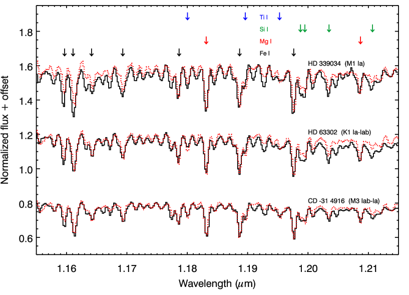
Figure 3: Examples of model fits (red dotted lines) to the data (black solid lines). Data have been resampled onto a 2$\times$ finer grid to help aid the identification of discrete spectral features. The top spectrum is an example of a poor fit, with reduced $\chi^{2}$=8.9. The middle spectrum is a “fair” fit, with $\chi^{2}$=4.5. The bottom spectrum has a good fit, with $\chi^{2}$=1.7.

2.3 Fitting procedure

Before comparing the observed and model spectra, we first degrade the spectral resolution of the model data to that of the observations using a gaussian convolution kernel. Then, in order to find the best-fit spectrum, we have experimented with several strategies. Firstly, we compare the normalized flux at each spectral channel and compute the reduced $\chi^{2}$ for each point in the model grid,

$$\chi^{2}=\frac{1}{\nu}\sum\displaystyle\left(\frac{f_{i,\rm obs}-f_{i,\rm mod}}{\sigma_{i}}\right)^{2}$$ (1)

where $f_{i,\rm obs}$ and $f_{i,\rm mod}$ are the observed and model fluxes at each wavelength channel $i$; $\sigma_{i}$ is the uncertainty in the flux, taken to be 0.01 at each channel (i.e. SNR=100); and $\nu$ is the number of degrees of freedom,

$$\nu=N-n-1$$ (2)

where $N$ is the number of wavelength channels, and $n$ is the number of model parameters being fitted. In the case of the MARCS grid, $n=3$ ($\log Z$, $T_{\rm eff}$, and $\xi$). We then take the best fitting model to be that point in the grid with the lowest value of $\chi^{2}$.

A second fitting method applies a similar principle, but this time instead of fitting the entire spectral region we fit only the equivalent widths (EWs) of the strongest spectral lines: those of Fe i (1.16108$\mu$m, 1.16414$\mu$m, 1.18866$\mu$m, 1.19763$\mu$m) and Mg i (1.18314$\mu$m, 1.20869$\mu$m). We again find the best fitting model by determining the point in the model grid with the lowest $\chi^{2}$. We estimate the typical uncertainty in EW measurements ($\sigma_{i}$) to be around 10%, from repeating EW measurements of lines and slightly varying the wavelength ranges.

The first ‘full-spectrum’ method has the advantage that it fits the whole spectrum, and so in principle can deal with blends of lines. The second ‘strong-lines’ method on the other hand takes into account only the most prominent spectral features and so is not swayed by unidentified blends for which the physical data may be poorly known. In practice, we settled on a method which is a hybrid of these two – we look at the residuals between the model and observed spectrum, as in the ‘full-spectrum’ method, but only at select regions of the spectrum. This allows us to place more emphasis on the strong lines, but also deal with blended lines such as the Fe i-Si i blend at 1.198$\mu$m.

To determine the best-fit physical properties and their respective uncertainties, we first find the point in the model grid with the lowest $\chi^{2}$, $\chi^{2}$_best. We then take into account all points in the grid with $\chi^{2}$-$\chi^{2}$${}_{\rm best}<\Delta$$\chi^{2}$, where $\Delta$$\chi^{2}$ is an arbitrary number. If there are fewer than 10 models within this range, we take the 10 models with the best $\chi^{2}$. We then compute the weighted mean of a physical property $\bar{X}$ and its uncertainty $\sigma\bar{X}$ from the relations,

$$\bar{X}=\frac{\sum^{N}_{i}w_{i}x_{i}}{\sum^{N}_{i}w_{i}},~{}~{}~{}\sigma\bar{X}=\sqrt{\frac{N^{\prime}}{N^{\prime}-1}\frac{\sum^{N}_{i}w_{i}(x_{i}-\bar{X})^{2}}{\sum^{N}_{i}w_{i}}}$$ (3)

where $x_{i}$ is that physical property (e.g. $T_{\rm eff}$, $\xi$, $\log Z$) in model $i$, and the weights $w_{i}$ are calculated from the $\chi^{2}$ of each model in the grid,

$$w_{i}=e^{-\chi^{2}/2}$$ (4)

and $N^{\prime}$ is the number of non-zero weights. The parameter which governs how many models are used in the computation of the physical parameters, $\Delta$$\chi^{2}$, is initially set to 2 (see also Mottram et al., submitted, for similar use of this analysis technique). However, we found that this significantly overestimated the errors, particularly in $\log Z$ (as will be discussed in Sect. 3), and we concluded that $\Delta$$\chi^{2}$=1 was more appropriate.

An example of this process is shown in Fig. 2, where we show $\chi^{2}$ contours in the $T_{\rm eff}$-$\log Z$ plane. The cross indicates the derived temperature and metallicity for one star in the sample. It can be seen from the figure that the inferred $\log Z$ has only a weak sensitivity to the fitted $T_{\rm eff}$.

Table 1: Derived parameters for the programme stars. Temperatures are those appropriate for their spectral types from the calibration of Levesque et al. (2005); where a star is between spectral types we linearly interpolate between the two. Abundance types are either ‘st’ for standard, or ‘CN’ for CN processed.

Name	Spec Type	T(K)	Tfit(K)	log[Z]	$\xi$/ km s-1	AbT	$\chi^{2}$
HD63302	K1Ia-Iab	4100	3660 $\pm$ 180	0.02 $\pm$ 0.20	3.4 $\pm$ 0.5	st	4.47
HD212466	K2O-Ia	4015	3770 $\pm$ 170	0.17 $\pm$ 0.20	3.8 $\pm$ 0.5	st	5.57
HD187238	K3Iab-Ib	4015	3630 $\pm$ 180	0.04 $\pm$ 0.21	2.3 $\pm$ 0.5	st	4.91
HD185622A	K4Ib	3928	3590 $\pm$ 170	0.12 $\pm$ 0.20	2.4 $\pm$ 0.5	st	5.95
HD216946	K5Ib	3840	3580 $\pm$ 230	-0.15 $\pm$ 0.27	2.5 $\pm$ 0.5	CN	3.29
HD14404	M1-Iab-Ib	3745	3580 $\pm$ 170	0.10 $\pm$ 0.19	2.5 $\pm$ 0.5	CN	4.45
HD39801	M1-M2Ia-Ia	3710	3520 $\pm$ 160	0.19 $\pm$ 0.21	2.3 $\pm$ 0.5	st	6.59
HD35601	M1.5Iab-Ib	3710	3630 $\pm$ 160	0.11 $\pm$ 0.19	2.8 $\pm$ 0.5	st	3.87
BD+60 265	M1.5Ib	3710	3570 $\pm$ 140	0.16 $\pm$ 0.17	2.3 $\pm$ 0.5	st	6.90
HD339034	M1Ia	3745	3820 $\pm$ 160	0.29 $\pm$ 0.15	3.5 $\pm$ 0.5	st	8.86
HD10465	M2Ib	3660	3520 $\pm$ 220	-0.08 $\pm$ 0.27	3.4 $\pm$ 0.6	st	1.78
HD14469	M3-M4Iab	3550	3530 $\pm$ 160	0.15 $\pm$ 0.22	2.4 $\pm$ 0.5	CN	5.76
CD-31 49	M3Iab-Ia	3605	3580 $\pm$ 220	-0.15 $\pm$ 0.29	3.1 $\pm$ 0.6	st	1.67
RW Cyg	M3toM4Ia-I	3550	3680 $\pm$ 180	0.31 $\pm$ 0.21	2.6 $\pm$ 0.5	st	6.98

As an additional check on the significance of each abundance measurement, we look at the $\log Z$ of the models in the grid with $T_{\rm eff}$$\pm$200K and $\xi\pm$1 km s^-1. In each extreme, we determine the ‘best-fit’ $\log Z$ from the model with the lowest $\chi^{2}$. Therefore, we derive a range of $\log Z$ values by varying $T_{\rm eff}$ and $\xi$. In the vast majority of cases, we find that the range in $\log Z$ is less than the sampling of the model grid (0.25dex), and in the worst case two grid points ($\pm$0.25dex). This is smaller than the typical uncertainties on each measurement (see next Section).

3 Results

Before moving on to the derived stellar parameters for the programme stars, we first give examples of the quality of fits we achieve. In Fig. 3 we show the range of fits obtained, from the worst to the best. In the case of the worst fit (HD 339034, top spectrum in Fig. 3), it is clear that in the most part the strongest lines, those of Fe i and Mg i, are still matched very well, apart from at the blue end of the displayed spectrum where there may be a problem with the continuum normalization. The deficiencies come mainly from unresolved and unidentified blends, such as that at 1.194$\mu$m, and from the Si i lines. However, at higher spectral resolution the Si i lines would be unblended and could be incorporated into the fitting procedure, possibly obtaining much better fits (as will be shown in Sect. 4.2). A thorough examination of this requires higher resolution data and is left for a future study.

The other stars in Fig. 3 are fit very well by the procedure. This quality of fit is more typical of the results, as can be seen from the last column of Table LABEL:tab:averesults.

Figure 4: Results of the analysis process on the programme stars, as a function of their temperatures inferred from their literature spectral types and the temperature calibration scale of Levesque et al. (2005). The top panel shows the difference in $T_{\rm eff}$ between the literature values and that derived by the fitting procedure. The bottom panel shows the derived average metal content $\log Z$. The weighted means of each parameter are shown in the panels.

3.1 Derived stellar parameters

We now address the results of the fitting procedure across all stars studied. The temperatures, microturbulent velocities and average abundances for each star are listed in Table LABEL:tab:averesults. In Fig. 4 we show the values of $T_{\rm eff}$ and $\log Z$ derived for each star, as well as the averages of each parameter, as a function of the stars’ literature temperatures, assuming the temperature scale of Levesque et al. (2005). In terms of temperature, we find generally acceptable agreement with the literature values. We do find on average that the temperatures we derive are cooler by $\approx$150K, with a 1$\sigma$ standard deviation of 170K on the distribution. This effect is more pronounced at higher temperatures. However, if one takes the old temperature scale from Humphreys & McElroy (1984), which are on average $\sim$200K cooler than those of Levesque et al., the agreement is almost perfect. This is curious, as the RSG temperature scale was rederived from the current generation of MARCS model atmospheres, but concentrating mainly on the $R$ and $I$ spectral windows. We will discuss how the derived temperature may be affected by line blending in Sect. 4, but we will also show in Sect. 3.2 that the fitted stellar temperature has very little impact on the measured abundances, so for now we are not concerned by this minor discrepancy.

The fitted values of $\log Z$ are very tightly distributed around zero, with mean metallicity of $\log Z$=$0.13\pm 0.14$, where the uncertainty again is the 1$\sigma$ standard deviation. These values are therefore consistent with Solar metal abundances, which is a reassuring result for a sample of objects in the Solar neighbourhood. If we assume for the moment that all objects in the sample have $\log Z$=0.0, then the bottom panel of Fig. 4 serves to illustrate an empirical determination of the precision of our analysis method, that is that we are deriving abundances accurate to $\pm$0.14dex. However, there is likely some intrinsic spread in the metallicities of the objects in our sample, so this value is an upper limit to the experimental uncertainty. This compares to the average errors we determined in the fitting process of $\sim$0.2dex (see column 4 of Table LABEL:tab:averesults). So, it is likely that our analysis process overestimates the experimental errors slightly. When we used $\Delta$$\chi^{2}$=2 in the fitting process (see previous Section) these errors were higher still, at around $\pm$0.25-0.3dex, yet the average $\log Z$ and its standard deviation were the same as with $\Delta$$\chi^{2}$=1. This is the reason we opted for $\Delta$$\chi^{2}$=1 during the fitting, since the errors were more comparable to ‘empirical’ error of $\pm$0.14dex. This level of precision is as good as any other abundance measurement technique.

For the microturbulent velocities $\xi$, all measured values are between 2-4 km s^-1, with an average of $2.8\pm 0.5$ km s^-1. This is a typical value for RSGs (see e.g. Davies et al., 2009b; Cunha et al., 2007). We note however that the $\xi$-sampling of the MARCS grid is very coarse, with computed models at 2 and 5 km s^-1 only. Our grid points at 3 and 4 km s^-1 were simple linear interpolations in between the computed models, and so if non-linear effects are present there will be a systematic uncertainty in our derived values of $\xi$. However, we can say that the current $\xi$-sampling of the model grid encompasses the range of values expected from the RSGs in our sample. The impact of the uncertainty in $\xi$ on abundance measurements will be explored in the next Section.

We explored two sets of models with different CNO mixtures – the ‘standard’ set, and the CNO-processed set with depleted C and enhanced N. For the majority of the objects studied the standard CNO abundance models provided the best fits. As with $\xi$, our sensitivity to this free parameter will be explored next.

Figure 5: The impact of fixing various input parameters on the results of the fitting process. Each panel shows the results of the best fit (i.e. letting all parameters vary), fixing $\xi$=2 km s^-1 and $\xi$=4 km s^-1, fixing the CNO elemental abundances to the ‘standard’ and ‘processed’ values, and fixing $\log g$=+1.0. The top panel shows the weighted-mean abundance level of all stars and its standard deviation. The bottom panel shows the median $\chi^{2}$ of all fits from each of the fitting methods.

3.2 Robustness of abundance measurements

In the previous Section we have shown that the abundances we measure in this technique are extremely consistent with the expected values, with a very high level of precision. To investigate the robustness of these measurements, we now explore the effect of varying the free parameters on the results. In Fig. 5 we plot the weighted mean of all stars’ fitted abundance levels, the standard deviation on this value, and the reduced $\chi^{2}$ values when forcing each of the model input parameters to be fixed.

Sensitivity to microturbulence

This parameter affects the EWs of strong lines. If lines are saturated, then by adding a degree of microturbulence the overall capacity to absorb is increased, and stronger absorption lines are observed. The second and third points on the $y$-axis in Fig. 5 show the impact of forcing the fitting routine to find the best fit when the microturbulence is fixed at $\xi$=2 km s^-1 and $\xi$=4 km s^-1. A systematic effect on the derived $\log Z$ can be seen, that is for lower $\xi$, higher $\log Z$ is found. However, the difference is small ($\pm$0.2dex), while larger dispersion in $\log Z$ is found, illustrated by the size of the error bar. The larger dispersion indicates that, on average, poorer fits are found, in accordance with the larger values of $\chi^{2}$ from the fitting procedure (bottom panel of Fig. 5). The small change in the average $\log Z$ suggests that the uncertainties in abundance levels propagated through from uncertainties in $\xi$ are typically less than the experimental error in $\log Z$.

Sensitivity to CNO abundances

We find very little sensitivity to this input parameter. Whether the ‘standard’ or ‘CNO processed’ abundances are used, the derived $\log Z$ is very close to the best-fit value, with similar error-bar (see the fourth and fifth points on the $y$-axis in Fig. 5).

Sensitivity to gravity

It is not possible as yet to make as thorough an investigation of the effect of varying this parameter as for the others, as it is poorly sampled in the MARCS grid for supergiants. However, models do exist for $\log g$=+1.0 and 0.0. These values probably bracket the accepted values for most RSGs, with $\log g$=0.0 being the most commonly used number (Lambert et al., 1984; Carr et al., 2000; Levesque et al., 2005; Cunha et al., 2007). Though values of $\log g$ as low as -0.5 have been measured for some RSGs, the vast majority of RSGs have gravities of $\log g$=0.0 and higher (see Fig. 5 of Cunha et al., 2007). We find that, on average the $\log g$=+1.0 fits produce significantly larger $\chi^{2}$, and a slightly larger spread on the $\log Z$ distribution. The average $\log Z$ however remains consistent with the best-fit solution to within the errors. We experimented with using the $\log g$=+1.0 models in the formal fitting procedure, and deriving best-fit values for $\log g$ rather than assuming a blanket value of $\log g$=0.0. In all cases we found that the derived values of $\log g$ were between 0.0 and 0.2, with negligible effect on the derived $\log Z$ and $T_{\rm eff}$.

Sensitivity to input $T_{\rm eff}$

The top panel of Fig. 5 illustrates that, for any set of model parameters used, we consistently derive temperatures that are systematically lower than the literature values, especially for earlier spectral types. As commented upon earlier, this may be due in part to the recently-rederived temperature scale for RSGs. Nevertheless, to investigate the significance of this effect we re-ran the fitting procedures but this time forced the fitted temperature to be the same as the literature temperatures, allowing the rest of the parameters to vary. The results are shown in the right-most points of Fig. 5. Though the reduced $\chi^{2}$ values are slightly worse than for any of the other model runs, the average abundances are again extremely consistent with the best-fit model, only with a slightly larger dispersion.

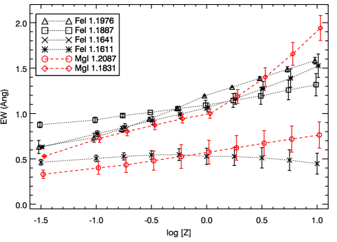
Figure 6: The effect of average metal content $\log Z$ on the EWs of the diagnostic lines used in this study, as measured from the synthetic spectra in the MARCS model grid. Points show the average EWs, while error bars show the range of EWs measured across the effective temperature range of RSGs (3400-4000K). All models use $\log g$=0.0, $\xi$=3 km s^-1, and standard CNO abundances. The $x$-values of each of the curves have been slightly offset from one another for clarity.

From this analysis, it appears that the free parameters the fitting process, namely $T_{\rm eff}$, $\xi$, $\log g$, and $X(\rm CNO)$, have very little effect on the derived abundances. The standard deviation on the results of each model run in Fig. 5 is only 0.2dex, with a mean of +0.0dex. These numbers are comparable to those derived for the ‘best-fit’ results. Thus, it seems that any systematic uncertainty in the fitting process is only comparable to the random error, and the derived abundance level is robust to fluctuations in the model’s free parameters.

4 Discussion

4.1 RSGs as abundance probes

The results of this study suggest that the MARCS model atmospheres provide excellent fits to the $J$-band spectra of Solar-neighbourhood RSGs. Moreover, the derived abundances seem to be relatively insensitive to the model input parameters $T_{\rm eff}$, $\log g$, $\xi$ and the mix of CNO abundances. Therefore, by constraining these input parameters to the ranges that are known to be valid for RSGs, it should be possible to derive metal abundances for RSGs to a precision of 0.1dex using medium resolution $J$-band spectroscopy.

To illustrate the sensitivity of the $J$-band diagnostic lines to average metal content, in Fig. 6 we plot the strengths of the strong lines identified in Sect. 2.3 as a function of $\log Z$ for the model spectra in the MARCS grid. The error-bars indicate the minimum and maximum EWs observed across the range of RSG temperatures, from 3400 to 4000K. All measurements were computed from the $\log g$=0.0, $\xi$=3 km s^-1 models with standard CNO abundances. The plot shows that, for these lines, there is very little variation with RSG spectral type, presumably due to the narrow range of temperatures that RSGs span. By contrast, the effect of changing metal content is much more pronounced. For the typical abundance gradient in a spiral galaxy of 0.05-0.2dex/kpc (see Garnett et al., 1997; Kudritzki et al., 2008; Bresolin et al., 2009; U et al., 2009), the strengths of these lines could increase by $\sim$50% between the innermost and outermost regions. As such variations in line strength would be easily detectable, RSGs could be powerful tools with which to study abundance trends in their host galaxies.

Table 2: Derived parameters for the two stars for which higher spectral resolution was available.

Name	Spec Type	$T$(K)	$T_{\rm fit}$(K)	$\log Z$	$\xi$( km s-1)
$\alpha$ Her	M5 Ib	3450	3460$\pm$220	-0.26$\pm$0.22	3.9$\pm$0.3
$\alpha$ Ori	M1.5 Iab	3710	3660$\pm$170	0.24$\pm$0.22	4.4$\pm$0.5

4.2 Benefits of increased spectral resolution

The spectra studied here were taken from the IRTF spectral library, the spectral resolution of which is $R=2000$. At this resolution we have identified six spectral lines which have sufficient strength to be largely unaffected by blending. Nevertheless, there is clearly some blending present between the metallic lines, e.g. those of Fe i and Ti i. At lower metallicities, where the metallic lines will tend to have lower EWs, blending may begin to introduce problems.

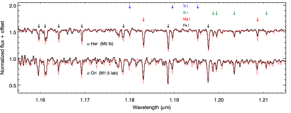
Figure 7: Best fits to the $J$-band spectrum of $\alpha$ Her and $\alpha$ Ori, with spectral resolution $R=6000$, published in Wallace et al. (2000). See text for details.

However, at greater spectral resolution the blending of the major lines is greatly reduced, increasing the number of strong diagnostic lines that may be studied, as well as increasing the number of elements that can be probed. This is illustrated in Fig. 7, where we plot the spectra of $\alpha$ Her and $\alpha$ Ori originally presented in Wallace et al. (2000). At this spectral resolution of $R=6000$ we see the lines of Si i and Ti i as unblended from the Fe i lines, particularly at 1.189$\mu$m and 1.198$\mu$m. The results of the fitting process for these two stars are shown in Table LABEL:tab:r3000. Note that the abundance measured for $\alpha$ Ori of $\log Z$=+0.24$\pm$0.22 is entirely consistent with the results of Lambert et al. (1984, Fe/H$\approx$+0.1)

The benefits of this are twofold. Firstly, it is possible to add the Si i and Ti i lines to the list of ‘strong features’ that are measured during the fitting process, enabling a more robust fit and determination of stellar temperature. For example, using only the Fe i and Mg i lines in the fitting procedure, we measure a temperature for $\alpha$ Ori of $T_{\rm eff}$=3300$\pm$200K. However, these fits underestimate the strengths of the Si i lines, as in the case of HD 212466 (see Sect. 3). When the Si i and Ti i lines are folded into the analysis we measure $T_{\rm eff}$=3660$\pm$170K, which is much closer to the temperature appropriate for its spectral type (M1.5 Iab, $T_{\rm eff}$=3710K, using the calibration of Levesque et al., 2005). We note however that the derived metallicity is relatively insensitive to this effect, changing by only $\sim$0.1dex.

Secondly, at increased spectral resolution the number of metallic elements that it is possible to investigate is greater. By studying the combined abundances of Mg, Si and Ti, combined with more detailed modelling, it should be possible to make a quantitative comparison of the relative abundances of Fe-group and $\alpha$-group elements, a key diagnostic of a galaxy’s star-forming history. Though the spectra we show in Fig. 7 have resolution of $R=6000$, we have found that it is still possible to separate the spectral lines at resolution of only $R=3000$. As lower resolutions mean shorter exposure times for objects of a given brightness, the limiting distance at which RSGs could be studied in this way is increased.

4.3 Extragalactic potential

The potential of RSGs as extragalactic abundance probes is enormous. With absolute magnitudes of $M_{J}\sim-8$ to $-11$ mag and very characteristic colors ( $V-I\approx 2.0$ mag) they can easily be detected as individual objects in galaxies at large distances. Using new IR multi-object spectrographs such as KMOS at the ESO VLT or MOSFIRE at Keck one will be able to reach limiting magnitudes of $M_{J}\approx 19$ mag with a spectral resolution of $R$=3000 and a signal-to-noise of 100 in long exposure sequences (for instance, totalling two nights). In this way quantitative spectroscopy of RSGs out to 10 Mpc distances will be possible allowing precise chemical abundances of galaxies to be determined and the evolution of galaxies to be disentangled.

The future, with next generation of 30m+ ground-based telescopes and the James Webb Space Telescope, is even more promising. These new facilities will be optimized for very high spatial resolution observations in the IR, so that the gain in limiting fluxes for multi-object spectrographs increases with the fourth power of aperture diameter. For instance, using the E-ELT exposure time estimator and including the dramatic effects of adaptive optics we will be able to go down $M_{J}\approx 22$ mag, which will give us a limiting distance of 30 Mpc. This opens up a truly remarkable volume of the local universe for very detailed and precise studies of the formation and chemical evolution of entire galaxy clusters, such as Virgo, Fornax, Puppis and Eridanus.

5 Conclusions

To demonstrate that it is possible to get accurate and precise abundance measurements from Red Supergiants (RSGs) at modest spectral resolutions of $R$=2-3000, we have studied a sample of RSGs in the Solar neighbourhood in conjunction with the latest MARCS model atmospheres. With no a priori assumptions about stellar parameters, we derive chemical abundances for each object which are close to the Solar value, with a mean abundance for the whole sample of 0.13$\pm$0.14dex. This dispersion in the mean is notwithstanding any intrinsic spread inherent in the sample, and is indicative of our experimental uncertainty. The level of precision achieved by this method is therefore as good as any other abundance indicator. We find that the derived abundance levels are relatively insensitive to the other model parameters of effective temperature, microturbulent velocity, CNO mixture and surface gravity, though the effects of very low surface gravities ($\log g$$<$0.0) have not been investigated here.

Though we do find effective temperatures which are on average lower than the literature values by $\sim$100-200K, this has very little impact on the derived abundances since $\log Z$ is extremely insensitive to $T_{\rm eff}$. Forcing the fitted temperature to be the same as the literature temperature for each star resulted in output abundances that were very similar and within the errors of the best fits. Furthermore, we argue that this $T_{\rm eff}$ discrepancy may be solved at resolutions of $R>3000$ when the blending of key diagnostic lines is diminished.

The results of our work therefore suggest that it is possible to obtain accurate abundance information at spectral resolutions which are much lower than commonly used at present. This opens the door for abundance studies of entire galaxies at infrared wavelengths, out to distances of several Mpc.

As for the future, we will shortly present an analysis of a sample of RSGs from the two Magellanic Clouds, showing that this technique can be applied across a large range of metallicities. We are also in the process of expanding the model grid to include a broader range of gravities, better sampling in $\xi$-space, and with accurate synthetic spectra computed at high resolution.

References

- Bresolin et al. (2009) Bresolin, F., Gieren, W., Kudritzki, R., Pietrzyński, G., Urbaneja, M. A., & Carraro, G. 2009, ApJ, 700, 309
- Carr et al. (2000) Carr, J. S., Sellgren, K., & Balachandran, S. C. 2000, ApJ, 530, 307
- Chiavassa et al. (2009) Chiavassa, A., Plez, B., Josselin, E., & Freytag, B. 2009, A&A, 506, 1351
- Cunha et al. (2007) Cunha, K., Sellgren, K., Smith, V. V., Ramirez, S. V., Blum, R. D., & Terndrup, D. M. 2007, ApJ, 669, 1011
- Davies et al. (2009a) Davies, B., Origlia, L., Kudritzki, R., Figer, D. F., Rich, R. M., & Najarro, F. 2009a, ApJ, 694, 46
- Davies et al. (2009b) Davies, B., Origlia, L., Kudritzki, R., Figer, D. F., Rich, R. M., Najarro, F., Negueruela, I., & Clark, J. S. 2009b, ApJ, 696, 2014
- Garnett et al. (1997) Garnett, D. R., Shields, G. A., Skillman, E. D., Sagan, S. P., & Dufour, R. J. 1997, ApJ, 489, 63
- Gustafsson et al. (2008) Gustafsson, B., Edvardsson, B., Eriksson, K., Jørgensen, U. G., Nordlund, Å., & Plez, B. 2008, A&A, 486, 951
- Humphreys & McElroy (1984) Humphreys, R. M. & McElroy, D. B. 1984, ApJ, 284, 565
- Josselin & Plez (2007) Josselin, E. & Plez, B. 2007, A&A, 469, 671
- Kewley & Ellison (2008) Kewley, L. J. & Ellison, S. L. 2008, ApJ, 681, 1183
- Kudritzki et al. (2008) Kudritzki, R., Urbaneja, M. A., Bresolin, F., Przybilla, N., Gieren, W., & Pietrzyński, G. 2008, ApJ, 681, 269
- Kudritzki (2010) Kudritzki, R. P. 2010, ArXiv e-prints
- Lambert et al. (1984) Lambert, D. L., Brown, J. A., Hinkle, K. H., & Johnson, H. R. 1984, ApJ, 284, 223
- Levesque et al. (2005) Levesque, E. M., Massey, P., Olsen, K. A. G., Plez, B., Josselin, E., Maeder, A., & Meynet, G. 2005, ApJ, 628, 973
- Meynet & Maeder (2000) Meynet, G. & Maeder, A. 2000, A&A, 361, 101
- Origlia et al. (2004) Origlia, L., Ranalli, P., Comastri, A., & Maiolino, R. 2004, ApJ, 606, 862
- Plez (2008) Plez, B. 2008, Physica Scripta Volume T, 133, 014003
- Rayner et al. (2009) Rayner, J. T., Cushing, M. C., & Vacca, W. D. 2009, ApJS, 185, 289
- Schwarzschild (1975) Schwarzschild, M. 1975, ApJ, 195, 137
- U et al. (2009) U, V., Urbaneja, M. A., Kudritzki, R., Jacobs, B. A., Bresolin, F., & Przybilla, N. 2009, ApJ, 704, 1120
- Wallace et al. (2000) Wallace, L., Meyer, M. R., Hinkle, K., & Edwards, S. 2000, ApJ, 535, 325