Stochastic backgrounds of gravitational waves from extragalactic sources

Abstract

Astrophysical sources emit gravitational waves in a large variety of processes occurred since the beginning of star and galaxy formation. These waves permeate our high redshift Universe, and form a background which is the result of the superposition of different components, each associated to a specific astrophysical process. Each component has different spectral properties and features that it is important to investigate in view of a possible, future detection. In this contribution, we will review recent theoretical predictions for backgrounds produced by extragalactic sources and discuss their detectability with current and future gravitational wave observatories.

1 Introduction

A stochastic background of gravitational waves (GWs) is expected to arise as a super-position of a large number of unresolved sources, from different directions in the sky, and with different polarizations. It is usually described in terms of the GW spectrum,

$$\Omega_{\rm GW}=\frac{f}{\rho_{\rm cr}}\frac{d\rho_{\rm GW}}{df},$$

where $d\rho_{\rm GW}$ is the energy density of GWs in the frequency range $f$ to $f+df$ and $\rho_{\rm cr}$ is the critical energy density of the Universe.

Stochastic backgrounds of GWs are interesting to investigate because they (i) represent a foreground signal for the detection of primordial backgrounds (see the contribution of M. Maggiore in this conference), and (ii) provide important information on GW sources and on the properties of distant stellar populations.

The starting point in any calculation of the GW backgrounds produced by extragalactic sources is the redshift evolution of the comoving star formation rate density. This is generally inferred from observations which have been recently extended out to redshifts $z\sim 10$ following the analysis of the deepest near-infrared image ever obtained on the Hubble Ultra Deep Field using the new/IR camera on HST (Bouwens et al. 2010). The detection of galaxies at $z=8.4-10$, just 500-600 Myr after recombination and in the heart of the reionization epoch, provides clues about galaxy build-up at a time that must have been as little as 200-300 Myr since the first substantial star formation (at $z\sim 15-20$). The existence of galaxies at $z\sim 10$ shows that galaxy formation was well underway at this very early epoch.

2 GW backgrounds from extragalactic sources: early predictions

The most interesting astrophysical sources of gravitational radiation such as the core-collapse of a massive star to a black hole, the instabilities of a rapidly rotating neutron star or the inspiral and coalescence of a compact binary system are all related to the ultimate stages of stellar evolution. Thus, the rate of formation of these stellar remnants can be deduced from the rate of formation of the corresponding stellar progenitors once a series of assumptions are made regarding the stellar evolutionary track followed.

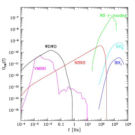
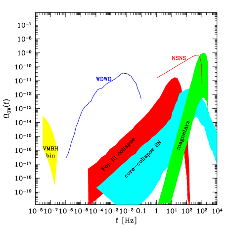
Figure 1: Left panel: collection of GW background signals for different sources, such as double neutron stars (NSNS) and white dwarfs (WDWD, Schneider et al. 2001), rapidly rotating neutron stars (NS r-modes, Ferrari et al. 1999b), black hole collapse assuming two possible values for the specific angular momentum (BH1, BH2, Ferrari et al. 1999a), collapse of super-massive stars to black hole (VMBH, Schneider et al. 2000). Right panel: collection of GW backgrounds predicted by additional studies for double neutron stars (NSNS, Regimbau & Chauvinaeu 2007), double white dwarfs (WDWD, Farmer & Phinney 2003), collapse of Population II (core-collapse SN) and III stars (Pop III collapse, Buonanno et al. 2005), magnetars (Regimbau & de Freitas Pacheco 2006), binary very massive black hole systems (VMBH bin, Sesana et al. 2008).

A few years ago we have published estimates of the stochastic backgrounds produced by astrophysical sources, concentrating in particular on the (i) gravitational collapse of a massive star that leads to the formation of a black hole (Ferrari, Matarrese & Schneider 1999a), (ii) the emission of GWs by newly born rapidly rotating neutron stars (Ferrari, Matarrese & Schneider 1999b), (iii) gravitational collapse of a super-massive star to black hole (Schneider et al. 2000), (iv) the orbital decay of various degenerate binary systems that loose angular momentum as a consequence of the emission of gravitational radiation (Schneider et al. 2001).

While to compute the first two classes of backgrounds we could simply derive the black holes and neutron stars formation rate as a function of redshift from the corresponding star formation rate (estimated from observational data) via an assumed stellar initial mass function (IMF), the last two classes required additional information from theoretical models for the evolution of primordial objects (VMBHs), and from a binary population synthesis model (compact binaries). We refer the interested reader to the original papers for further details. The resulting GW backgrounds are presented in the left panel of Fig. 1. In the right panel of the same figure, we also show a collection of signals predicted by additional studies on double compact stellar binaries (Farmer & Phinney 2003; Regimbau & Chauvineau 2007), on the collapse of Population II and III stars (Buonanno et al. 2005), on strongly magnetized neutron stars (Regimbau & de Freitas Pacheco 2006), and on very massive black hole binary systems (Sesana, Vecchio & Colacino 2008). Shaded regions illustrate the sensitivity of the corresponding signal to variations of critical parameters.

3 GW backgrounds from Population III and II stars

Our present understanding of Pop III star formation suggests that these stars are not necessarily confined to form in the first dark matter halos at redshift $z>20$ but may continue to form during cosmic evolution in regions of sufficiently low metallicity, with $Z<Z_{\rm cr}=10^{-5\pm 1}Z_{\odot}$. At these low metallicities, the reduced cooling efficiency and large accretion rates favor the formation of massive stars, with characteristic masses $\geq 100M_{\odot}$ (Bromm et al. 2001; Schneider et al. 2002, 2006a; Omukai et al. 2005). With the exception of the dynamical range $(140-260)M_{\odot}$, where they are expected to explode as pair-instability SNe (Heger & Woosley 2002), these stars are predicted to collapse to black holes of comparable masses and thus to be efficient sources of GWs. Earlier estimates of the extragalactic background generated by the collapse of the first stars, discussed in the previous section, were limited by our poor understanding of their characteristic masses and formation rates. In particular, the Pop III star formation rate and the cosmic transition between Pop III and Pop II stars is regulated by the rate at which metals are formed and mixed in the gas surrounding the first star forming regions, a mechanism that we generally refer to as chemical feedback.

Semi-analytic studies which implement chemical feedback generally find that, due to inhomogeneous metal enrichment, the transition is extended in time, with coeval epochs of Pop III and Pop II star formation, and that Pop III stars can continue to form down to moderate redshifts, $z<5$ (Scannapieco, Schneider & Ferrara 2003; Schneider et al. 2006b). To better assess the validity of these semi-analytic models, Tornatore, Ferrara & Schneider (2007) have performed a set of cosmological hydrodynamic simulations with an improved treatment of chemical enrichment. In the simulation, it is possible to assign a metallicity-dependent stellar IMF. When $Z>Z_{\rm cr}$ Pop II stars are assumed to form according to a Salpeter IMF $\Phi(M)\propto M^{-(1+x)}$ with $x=1.35$ and lower (upper) mass limit of $0.1M_{\odot}$ ($100M_{\odot}$). Stars with masses in the $8-40M_{\odot}$ range explode as Type-II SNe and the explosion energy and metallicity-dependent metal yields are taken from Woosley & Weaver (1985). Stars with masses $>40M_{\odot}$ do not contribute to metal enrichment as they are assumed to directly collapse to black holes. Very massive Pop III stars form in regions where $Z<Z_{\rm cr}$; since theoretical models do not yet provide any indication on the shape of the Pop III IMF, Tornatore et al. (2007) adopt a Salpeter IMF shifted to the mass range $100-500M_{\odot}$; only stars in the pair-instability range ($140-260M_{\odot}$) contribute to metal-enrichment and the metal yields and explosion energies are taken from Heger & Woosley (2002). The simulation allows to follow metal enrichment properly accounting for the finite stellar lifetimes of stars of different masses, the change of the stellar IMF and metal yields. The numerical schemes adopted to simulate metal transport ad diffusion are discussed in Tornatore et al. (2007) to which we refer the interested reader for more details.

The top panel in Fig. 2 shows the redshift evolution of the cosmic star formation rate and the contribution of Pop III stars predicted by the simulation. In this model, the critical metallicity which defines the Pop III/Pop II transition is taken to be $Z_{\rm cr}=10^{-4}Z_{\odot}$, at the upper limit of the allowed range. However, additional runs show that decreasing the critical metallicity to $10^{-6}Z_{\odot}$ reduces the Pop III star formation rate by a factor $<10$. It is clear from the figure that Pop II stars always dominate the cosmic star formation rate; however, in agreement with previous semi-analytic studies, the simulation shows that Pop III stars continue to form down to $z<5$, although with a decreasing rate. Over cosmic history, the fraction of baryons processed by Pop III stars is predicted to be $f_{b}=2\times 10^{-6}$.

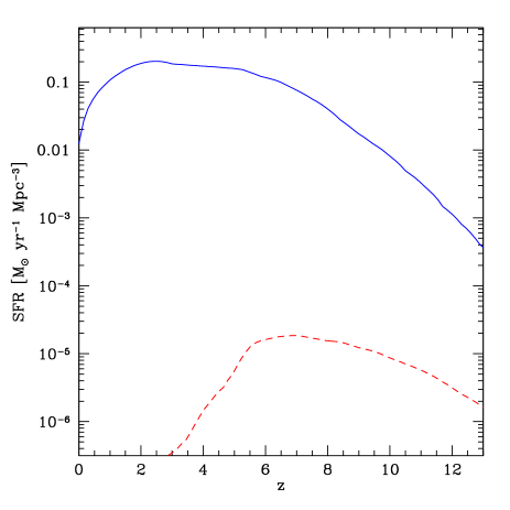
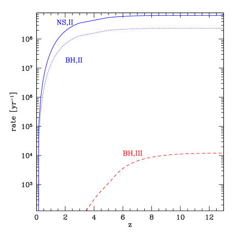
Figure 2: Left panel: redshift evolution of the comoving star formation rate density (solid lines). The dotted line shows the contribution of Pop III stars (see text). Right panel: redshift evolution of the number of gravitational wave sources formed per unit time within a comoving volume. The top curves show the contribution of Pop II stars leaving behind neutron stars (NS,II solid line) and black holes (BH,II dotted); the bottom dotted line represents the contribution of Pop III stars collapsing to black holes (BH,III dashed).

3.1 GW emission from $[8-20]M_{\odot}$ Pop II stars

The first class of sources we have considered are core-collapse SNe leaving behind a NS remnant. To model the GW emission from these sources we have used the waveforms predicted by Muller et al. (2004) using sophisticated 2D numerical simulations with a detailed implementation of neutrino transport and neutrino-matter interactions. In particular, we adopt as our template spectrum that of a rotating 15 $M_{\odot}$ star which also gives the most optimistic GW signals, which corresponds to a GW emission efficiency of $1.8\times 10^{-8}M_{\odot}c^{2}$. The waveform is shown in the upper left panel of Fig. 3.

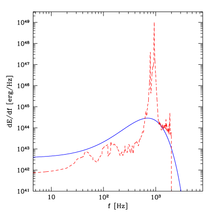
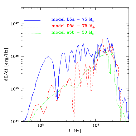
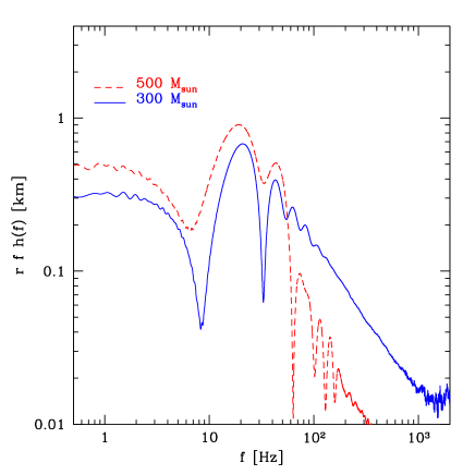
Figure 3: Upper left panel: template GW energy spectrum for core collapse to neutron stars. The solid line is the rotating 15 $M_{\odot}$ progenitor model of Muller et al. (2004), the dashed line is the g-mode spectrum for a 25 $M_{\odot}$ progenitor model of Ott et al. (2006). Upper right panel: template GW energy spectrum for core collapse to black holes. Three selected models from the analysis of Sekiguchi & Shibata (2005) are shown, which differ for the initial progenitor mass and equation of state. The resulting dynamical evolution and GW emission is different (see text). Lower panel: GW spectral distribution taken from Suwa et al. (2007) for two different template progenitor models with $300$ and $500M_{\odot}$.

As an alternative upper limit to the GW emission associated to these sources we have also assumed as a template for our single source spectrum the waveform obtained by Ott et al. (2006); in this scenario, based on axisymmetric Newtonian core-collapse supernova simulations, the dominant contribution to gravitational wave emission is due to the oscillations of the protoneutron star core. These are predominantly g-modes oscillations, which are excited hundreds of milliseconds after bounce by turbulence and by accretion downstreams from the SN shock (undergoing the Standing-Accretion-Shock-Instability, SASI), and typically last for several hundred milliseconds. In this phase a strong GW emission has been shown to occur, with a corresponding energy ranging from $1.5\times 10^{-8}M_{\odot}c^{2}$ for a 11 $M_{\odot}$ progenitor, to $8.2\times 10^{-5}M_{\odot}c^{2}$ for a 25 $M_{\odot}$ progenitor. In the latter case, the largest emission is caused by the more massive iron core, higher post-bounce accretion rates and higher pulsation frequencies and amplitudes. In these models the contribution of the anisotropic neutrinos emission is found to be negligible. If we take the 25 $M_{\odot}$ progenitor model, we can assume this to be an upper limit to the GW emission from these sources. The corresponding waveform is also shown in the upper left panel of Fig. 3.

3.2 GW emission from $[20-100]M_{\odot}$ Pop II stars

Progenitors with masses between 20 and 100 $M_{\odot}$ may lead to a prompt collapse to BH or to the formation of a proto-neutron star that, due to signficant fall-back, will end its life as a black hole. To model the GW emission from these events we have used the results of numerical simulations performed in full GR by Sekiguchi & Shibata (2005) of a grid of rotating stellar cores resulting from the evolution of stellar progenitors with masses 50-100 $M_{\odot}$. We have selected three representative models: D5a and D5d are associated to 75 $M_{\odot}$ stars, A5b to a 50 $M_{\odot}$ star. These models, which are shown in the upper right panel of Fig. 3, also differ for the equations of state, which translate into distinct collapse dynamics. The gravitational energy emitted is typically in the range $[2-3]\times 10^{-7}M_{\odot}c^{2}$.

3.3 GW emission from $[100-140]M_{\odot}$ and $[260-500]M_{\odot}$ Pop III stars

The collapse of Pop III stars to black holes has been suggested to be a much more efficient source of GWs than todays’ SN population: according to 2D simulations of a zero-metallicity 300 $M_{\odot}$ stars which take the effects of GR and neutrino transport into account, the estimated total energy released in GWs ranges between $[2\times 10^{-4}-2\times 10^{-3}]M_{\odot}c^{2}$ (Suwa et al. 2007, Fryer et al. 2001), with a factor of ten discrepancy among the two analyses ascribed to different initial angular momentum distribution. Since we want to be conservatives, we take the gravitational waveforms predicted by the most recent analysis of Suwa et al. (2007) which we show in the lower panel of Fig. 3.

4 Results

In Fig. 4, we show the function $\Omega_{\rm GW}$ evaluated integrating the single source spectra described above over the corresponding rate evolution (Marassi, Schneider & Ferrari 2009),

$$\Omega_{\rm GW}(f)=\frac{f}{c^{3}\rho_{cr}}\left[\frac{dE}{dSdfdt}\right],$$

where $dE/(dSdfdt)$ is the spectral energy density of the stochastic background,

$$\frac{dE}{dSdfdt}=\int^{z_{f}}_{0}\int^{M_{f}}_{M_{i}}dR(M,z)\big{<}\frac{dE}{dSdf}\big{>},$$

$dR(M,z)$ is the differential source formation rate,

$$dR(M,z)=\frac{\dot{\rho}_{\star}(z)}{(1+z)}\frac{dV}{dz}\Phi(M)dMdz,$$

and $\big{<}\frac{dE}{dSdf}\big{>}$ is the locally measured average energy flux emitted by a source at distance $r$. For sources at redshift $z$ it becomes,

$$\big{<}\frac{dE}{dSdf}\big{>}=\frac{(1+z)^{2}}{4\pi d_{L}(z)^{2}}\frac{dE^{e}_{GW}}{df_{e}}[f(1+z)]$$

where $f=f_{e}(1+z)^{-1}$ is the redshifted emission frequency $f_{e}$, and $d_{L}(z)$ is the luminosity distance to the source. The redshift evolution of the GW source formation rates, integrated over the comoving volume element, are shown in the right panel of Fig. 2.

We see that below $\sim 10$ Hz the Pop III GWB dominates over the Pop II background; its maximum amplitude is $\Omega_{\rm GW}\simeq 10^{-14}$ at $f=2.74$ Hz. At larger frequencies the background produced by Pop II stars is much larger than that of Pop III. Stars with progenitors in the range (20-100)$M_{\odot}$ contribute with a nearly monotonically increasing behavior, reaching amplitudes $\Omega_{\rm GW}\simeq 4\times 10^{-10}$ at $f\in(759-850)$ Hz. For stars with progenitors in the range (8-25)$M_{\odot}$ the GWB has a shape which depends on the waveform used as representative of the collapse: that obtained using the waveform of Muller et al. (2004) is quite smooth and peaks at $f=387$ Hz, with amplitude $\Omega_{\rm GW}\simeq 10^{-12}$. The background obtained using waveforms produced by the core-collapse model of Ott et al. (2006), instead, is comparable in amplitude with those produced by more massive progenitors, reaching the maximum amplitude $\Omega_{\rm GW}\simeq 7\times 10^{-10}$ at $f=485$ Hz.

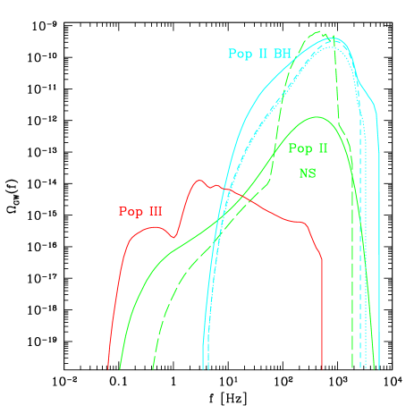
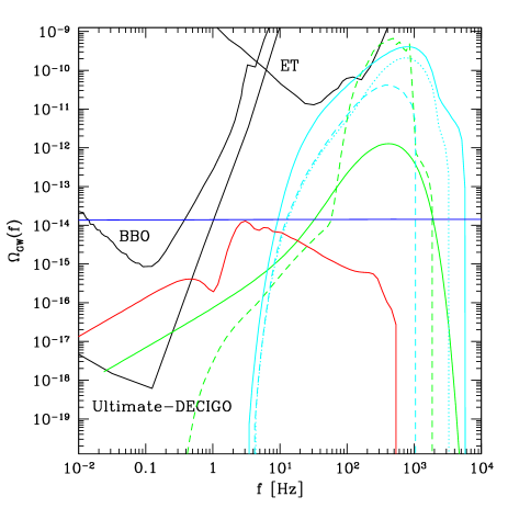
Figure 4: Left panel: the function $\Omega_{\rm GW}$ as a function of frequency for stochastic backgrounds associated to Pop III/II stars (see text). Right panel: same as in the left panel but applying the zero-frequency limit to the background signals where the gravitational wave emission below $1~{}Hz$ is dominated by the neutrino contribution. Superimposed on the astrophysical signals are the sensitivity curves for the next generation gravitational telescopes (BBO, Ultimate-DECIGO, ET) and the upper limit on the stochastic background generated during the inflationary epoch (see text).

In the right panel of Fig. 4, we have applied to the same signals the so-called zero-frequency limit: in fact, current numerical simulations describe the source collapse at most for a few seconds, and cannot predict the emission below a fraction of Hz. To evaluate the background in the low frequency region $f\leq$ 0.1 Hz, it is customary to extend the single source waveform $f|\tilde{h}(f)|$ to lower frequencies, where the emission is dominated by the neutrino signal. Superimposed on the predicted signals, we also show the foreseen sensitivity curves of the next generation of GW telescopes (BBO, Seto 2006; Ultimate-DECIGO, Kanda, private communication; ET, Regimbau, private communication). All the sensitivity curves are obtained assuming correlated analysis of the outputs of independent spacecrafts (or of different ground-based detectors). It is clear for the figure that BBO has no chance to detect the background signals produced by Pop III/Pop II stars; these signals, however, are within the detection range of Ultimate-DECIGO and are marginally detectable by ET.

The horizontal line in the same panel shows the upper limit on the stochastic background generated during the inflationary epoch taken from Abbott et al. (2009). Thus, the Pop III/II signals dominate over the primordial background only for frequencies $\geq 3$ Hz. Even below this frequency range, however, it may be possible to discriminate the astrophysical backgrounds from dominant instrumental noise or from primordial signals exploiting the non-Gaussian (shot-noise) structure of the former, which are characterized by duty-cycles of the order of $10^{-2}$ ($10^{-4}$) for Pop II (Pop III) sources (see Marassi et al. 2009).

In particular Seto (2008) has proposed a method to check if the detected GWB is an inflation-type background or if it is contaminated by undetectable weak burst signals from Pop III/Pop II collapse. If, in the future, it will be possible to extract information on the Pop III GWB component, we can have a tool to investigate the formation history of these first stars.

References

References

- [1] Andersson N. 1998, ApJ, 502, 708
- [2] Andersson N., Kokkotas K. & Schutz B. F. 1999, ApJ, 510, 846
- [3] Bouwens R. J. et al. 2010, ApJ, 709, 133
- [4] Buonanno A., Sigl G., Raffelt G. G., Janka H., Muller E., 2005, Phys. Rev. D, 72, 084001
- [5] Bromm V., Ferrara A., Coppi P.S., Larson R.B., 2001, MNRAS, 328, 969
- [6] Farmer A. J. & Phinney E. S. 2003, MNRAS, 346, 1197
- [7] Ferrari V., Matarrese S., Schneider R., 1999a, MNRAS, 303, 247
- [8] Ferrari V., Matarrese S., Schneider R., 1999b, MNRAS, 303, 258
- [9] Fryer C. L., Woosley S. E., Heger A., 2001, APJ 550, 372
- [10] Heger A., Woosley S. E., 2002, ApJ, 567, 532
- [11] Marassi S., Schneider R. & Ferrari V. 2009, MNRAS, 398, 293
- [12] Muller E., Rapp M., Buras R., Janka H. T., Shoemaker D. H., 2004, APJ 603, 221
- [13] Omukai K., Tsuribe T., Schneider R., Ferrara A., 2005, ApJ, 626, 627
- [14] Ott C. D., Burrows A., Dessart L., Livne E., 2006, PRL, 96 201102
- [15] Regimbau T. & Chauvineau B. 2007, Classical and Quantum Gravity, 24, 627
- [16] Regimbau T. & de Freitas Pacheco J. A. 2006, ApJ, 642, 455
- [17] Scannapieco E., Schneider R., Ferrara A., 2003, ApJ, 589, 35
- [18] Schneider R., Ferrara A., Ciardi B., Ferrari V., Matarrese S., 2000, MNRAS, 317, 385
- [19] Schneider R., Ferrari V., Matarrese S. & Portegies-Zwart S., 2001, MNRAS
- [20] Schneider R., Ferrara A., Natarajan P., Omukai K., 2002, ApJ, 571, 30
- [21] Schneider R., Omukai K., Inoue A. K., Ferrara A., 2006a, MNRAS, 369, 1437
- [22] Schneider R., Salvaterra R., Ferrara A., Ciardi B., 2006b, MNRAS, 369, 825
- [23] Sekiguchi Y. & Shibata M., Phys. Rev. D, 2005, 71, 084013
- [24] Seto N., 2006, Phys. Rev. D, 73, 063001
- [25] Seto N., 2008, APJ, 683, L95
- [26] Sesana A., Vecchio A. & Colacino C. N. 2008, MNRAS, 390, 192
- [27] Stark T. F. & Piran T. 1985, Phys. Rev. Lett., 55 891
- [28] Suwa Y., Takiwaki T., Kotake K., Sato K., 2007a, APJ 665, L43
- [29] Tornatore L., Ferrara, A., Schneider, R. 2007a, MNRAS, 382, 945
- [30] Woosley S.E., Weaver T.A., 1995, ApJ, 101, 181