Chemical composition of the old globular clusters NGC 1786, NGC 2210 and NGC 2257 in the Large Magellanic Cloud.

Abstract

This paper presents the chemical abundance analysis of a sample of 18 giant stars in 3 old globular clusters in the Large Magellanic Cloud, namely NGC 1786, NGC 2210 and NGC 2257. The derived iron content is [Fe/H]= –1.75$\pm$0.01 dex ($\sigma$= 0.02 dex),  –1.65$\pm$0.02 dex ($\sigma$= 0.04 dex) and  –1.95$\pm$0.02 dex ($\sigma$= 0.04 dex) for NGC 1786, NGC 2210 and NGC 2257, respectively. All the clusters exhibit similar abundance ratios, with enhanced values ($\sim$+0.30 dex) of [$\alpha$/Fe], consistent with the Galactic Halo stars, thus indicating that these clusters have formed from a gas enriched by Type II SNe. We also found evidence that r-process are the main channel of production of the measured neutron capture elements (Y, Ba, La, Nd, Ce and Eu). In particular the quite large enhancement of [Eu/Fe] ($\sim$+0.70 dex) found in these old clusters clearly indicates a relevant efficiency of the r-process mechanism in the LMC environment.

1 Introduction

In the last decade, the advent of the high resolution spectrographs mounted on the 8-10 m telescopes has allowed to extend the study of the chemical composition of individual Red Giant Branch (RGB) stars outside our Galaxy up to dwarf and irregular galaxies of the Local Group. Chemical analysis of RGB stars are now available for several isolated dwarf spheroidal (dSph) galaxies as Sculptor, Fornax, Carina, Leo I, Draco, Sextans and Ursa Minor (Shetrone, Coté & Sargent, 2001; Shetrone et al., 2003; Letarte et al., 2006) and the Sagittarius (Sgr) remnant (Bonifacio et al., 2000; Monaco et al., 2005, 2007; Sbordone et al., 2007). As general clue, these studies reveal that the chemical abundance patterns in the extragalactic systems do not resemble those observed in the Galaxy, with relevant differences in the [$\alpha$/Fe] , [Ba/Fe] and [Ba/Y] ratios, thus suggesting different star formation history and chemical evolution (see e.g. Venn et al., 2004; Geisler et al., 2007; Tolstoy, Hill & Tosi, 2009).

Unlike the dSphs, the irregular galaxies as the Large Magellanic Cloud (LMC) contain large amount of gas and dust, showing an efficient ongoing star-formation activity. The LMC globular clusters (GCs) span a wide age/metallicity range, with both old, metal-poor and young, metal-rich objects, due to its quite complex star formation history. Several events of star formation occurred: the first one $\sim$13 Gyr ago and 4 main bursts at later epochs, 2 Gyr, 500 Myr, 100 Myr and 12 Myr ago (Harris & Zaritsky, 2009). Until the advent of the new generation of spectrographs, the study of the chemical composition of the LMC stars was restricted to red and blue supergiants (Hill et al., 1995; Korn et al., 2000, 2002), providing information only about the present-day chemical composition. The first studies based on high resolution spectra of RGB stars (Hill et al., 2000; Johnson et al., 2006; Pompeia et al., 2008) provided first and crucial information about the early chemical enrichment and nucleosynthesis.

Of the $\sim$300 compact stellar clusters listed by Kontizas et al. (1990), metallicity determinations from Ca II triplet are available for some tens of objects (Olszewski et al., 1991; Grocholski et al., 2006) and only for 7 clusters high-resolution spectroscopic analysis have been carried out (Hill et al., 2000; Johnson et al., 2006). With the final aim of reconstructing the formation history of star clusters in the LMC, a few years ago we started a systematic spectroscopic screening of giants in a sample of LMC GCs with different ages.

In the first two papers of the series (Ferraro et al., 2006; Mucciarelli et al., 2008) we presented the chemical analysis of 20 elements for 4 intermediate-age LMC clusters (namely, NGC 1651, 1783, 1978, 2173). Moreover, Mucciarelli et al. (2009) discussed the iron content and the abundances of O, Na, Mg and Al for 3 old LMC clusters (namely NGC 1786, 2210 and 2257), discovering anticorrelation patterns similar to those observed in Galactic clusters. Here we extend the abundance analysis to additional 13 chemical elements in these 3 LMC clusters, also performing a detailed comparison with stellar populations in our Galaxy (both in the field and in globulars) and in nearby dSphs.

The paper is organized as follows: Section 2 presents the dataset and summarized the adopted procedure to derive radial velocities; Section 3 describes the methodology used to infer the chemical abundances; Section 4 discusses the uncertainties associated to the chemical abundances. Finally, Section 5 and  6 present and discuss the results of the chemical analysis.

2 Observational data

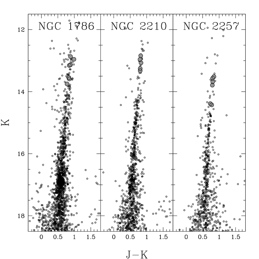
Figure 1: Color-Magnitude Diagrams in the (K, J-K) plane of the 3 LMC old clusters: grey points indicate the stars observed with FLAMES.

The observations were carried out with the multi-object spectrograph FLAMES (Pasquini et al., 2002) at the UT2/Kuyeen ESO-VLT (25-27 December 2007). We used FLAMES in the UVES+GIRAFFE combined mode, feeding 8 fibers to the UVES high-resolution spectrograph and 132 to the GIRAFFE mid-resolution spectrograph. The UVES spectra have a wavelength coverage between 4800 and 6800 $\mathring{A}$ with a spectral resolution of $\lambda/\Delta\lambda\sim$45000. We used the following GIRAFFE gratings: HR 11 (with a wavelength range between 5597 and 5840 $\mathring{A}$ and a resolution of $\sim$24000) and HR 13 (with a wavelength range between 6120 and 6405 $\mathring{A}$ and a resolution of $\sim$22000). These 2 setups have been chosen in order to measure several tens of iron lines, $\alpha$-elements and to sample Na and O absorption lines. Target stars have been selected on the basis of (K, J-K) Color-Magnitude Diagrams (CMDs), as shown in Fig. 1, from near infrared observations performed with SOFI@NTT (A. Mucciarelli et al. 2010, in preparation). For each exposure 2 UVES and a ten of GIRAFFE fibers have been used to sample the sky and allow an accurate subtraction of the sky level.

The spectra have been acquired in series of 8-9 exposures of $\sim$45 min each and pre-reduced independently by using the UVES and GIRAFFE ESO pipeline , including bias subtraction, flat-fielding, wavelength calibration, pixel re-sampling and spectrum extraction. For each exposure, the sky spectra have been combined together; each individual sky spectrum has been checked to exclude possible contaminations from close stars. Individual stellar spectra have been sky subtracted by using the corresponding median sky spectra, then coadded and normalized. We note that the sky level is only a few percents of the stars level, due to brightness of our targets, introducing only a negligible amount of noise in the stellar spectra. Note that the fibre to fibre relative transmission has been taken into account during the pre-reduction procedure. The accuracy of the wavelength calibration has been checked by measuring the position of some telluric OH and $O_{2}$ emission lines selected from the catalog of Osterbrock et al. (1996).

2.1 Radial velocities

Radial velocities have been measured by using the IRAF task FXCOR, performing a cross-correlation between the observed spectra and high S/N - high resolution spectrum of a template star of similar spectral type. For our sample we selected a K giant (namely HD-202320) whose spectrum is available in the ESO UVES Paranal Observatory Project database (Bagnulo et al., 2003). Then, heliocentric corrections have been computed with the IRAF task RVCORRECT. Despite the large number of availables fibers, only a few observed stars turned out to be cluster-member, due to the small size of the clusters within the FLAMES field of view. We selected the cluster-member stars according to their radial velocity, distance from the cluster center and position on the CMD. Finally, we identified a total of 7 stars in NGC 1786, 5 stars in NGC 2210 and 6 stars in NGC 2257. We derived average radial velocities of $V_{r}$= 264.3 km $s^{-1}$ ($\sigma$= 5.7 km $s^{-1}$), 337.5 km $s^{-1}$ ($\sigma$= 1.9 km $s^{-1}$) and 299.4 km $s^{-1}$ ($\sigma$= 1.5 km $s^{-1}$) for NGC 1786, 2210 and 2257, respectively. The formal error associated to the cross-correlation procedure is of $\sim$0.5–1.0 km $s^{-1}$. The derived radial velocities are consistent with the previous measures, both from integrated spectra (Dubath, Meylan & Mayor, 1997) and from low/high-resolution individual stellar spectra (Olszewski et al., 1991; Hill et al., 2000; Grocholski et al., 2006). In fact, for NGC 1786 Olszewski et al. (1991) estimated 264.4 km $s^{-1}$ ($\sigma$=4.1 km $s^{-1}$) from 2 giant stars, while Dubath, Meylan & Mayor (1997) provide a value of 262.6 km $s^{-1}$. For NGC 2210 the radial velocity provided by Olszewski et al. (1991) is of 342.6 km $s^{-1}$ ($\sigma$=7.8 km $s^{-1}$), while Dubath, Meylan & Mayor (1997) and Hill et al. (2000) obtained radial velocities of 338.6 and 341.7 km $s^{-1}$ ($\sigma$=2.7 km $s^{-1}$), respectively. For NGC 2257, Grocholski et al. (2006) provided a mean value of 301.6 km $s^{-1}$ ($\sigma$=3.3 km $s^{-1}$) and Olszewski et al. (1991) of 313.7 km $s^{-1}$ ($\sigma$=2.1 km $s^{-1}$). For all the targets Table 1 lists the S/N computed at 6000 $\mathring{A}$ for the UVES spectra and at 5720 and 6260 $\mathring{A}$ for the GIRAFFE-HR11 and -HR13 spectra, respectively. Also, we report $V_{r}$, dereddened $K_{0}$ magnitudes and $(J-K)_{0}$ colors and the RA and Dec coordinates (onto 2MASS astrometric system) of each targets.

3 Chemical analysis

Similarly to what we did in previous works (Ferraro et al., 2006; Mucciarelli et al., 2008, 2009), the chemical analysis has been carried out using the ROSA package (developed by R. G. Gratton, private communication). We derived chemical abundances from measured equivalent widths (EW) of single, unblended lines, or by performing a $\chi^{2}$ minimization between observed and synthetic line profiles for those elements (O, Ba, Eu) for which this approach is mandatory (in particular, to take into account the close blending between O and Ni at 6300.3 $\mathring{A}$ and the hyperfine splitting for Ba and Eu lines). We used the solar-scaled Kurucz model atmospheres with overshooting and assumed that local thermodynamical equilibrium (LTE) holds for all species. Despite the majority of the available abundance analysis codes works under the assumption of LTE, transitions of some elements are known to suffer from large NLTE effects (Asplund, 2005). Our Na abundances were corrected for these effects by interpolating the correction grid computed by Gratton et al. (1999).

The line list employed here is described in details in Gratton et al. (2003) and Gratton et al. (2007) including transitions for which accurate laboratory and theoretical oscillator strengths are available and has been updated for some elements affected by hyperfine structure and isotopic splitting. Eu abundance has been derived by the spectral synthesis of the Eu II line at 6645 $\mathring{A}$, in order to take into account its quite complex hyperfine structure, with a splitting in 30 sublevels. Its hyperfine components have been computed using the code LINESTRUC, described by Wahlgren (2005) and adopting the hyperfine constants A and B by Lawler et al. (2001) and the meteoritic isotopic ratio, being Eu in the Sun built predominantly through r-process. For sake of homogeneity we adopted the log gf by Biemont et al. (1982) already used in Mucciarelli et al. (2008) instead of the oscillator strength by Lawler et al. (2001). Ba II lines have relevant hyperfine structure components concerning the odd-number isotopes ¹³⁵Ba and ¹³⁷Ba, while the even-number isotopes have no hyperfine splitting; moreover, there are isotopic wavelength shifts between all the 5 Ba isotopes. In order to include these effects, we employed the linelist for the Ba II lines computed by Prochaska (2000) that adopted a r-process isotopic mixture. We note that the assumption of the r-process isotopic mixture instead of the solar-like isotopic mixture is not critical for the 3 Ba II lines analyzed here (namely, 5853, 6141 and 6496 $\mathring{A}$), because such an effect is relevant for the Ba II resonance lines (see Table 4 by Sneden et al., 1996).

For the La abundances we have not taken into account the hyperfine structure because the observed lines are too weak (typically 15-30 m$\mathring{A}$) and located in the linear part of the curve of growth where the hyperfine splitting is negligible, changing the line profile but preserving the EW. Abundances of V and Sc include corrections for hyperfine structure obtained adopting the linelist by Whaling et al. (1985) and Prochaska & McWilliam (2000).
In a few stars only upper limits for certain species (i.e. O, Al, La and Ce) can be measured. For O, upper limits have been obtained by using synthetic spectra (as described in Mucciarelli et al., 2009), while for Al, La and Ce computing the abundance corresponding to the minimum measurable EW (this latter has been obtained as 3 times the uncertainty derived by the classical Cayrel formula, see Section 3.1).

As reference solar abundances, we adopted the ones computed by Gratton et al. (2003) for light Z-odd, $\alpha$ and iron-peak elements, using the same linelist employed here. For neutron-capture elements (not included in the solar analysis by Gratton et al., 2003) we used the photospheric solar values by Grevesse & Sauval (1998). All the adopted solar values are reported in Tables 3, 4 and 5.

3.1 Equivalent Widths

All EWs have been measured by using an interactive procedure developed at our institute. Such a routine allows to extract a spectral region of about 15-25 $\mathring{A}$ around any line of interest. Over this portion of spectrum we apply a $\sigma$-rejection algorithm to remove spectral lines and cosmic rays. The local continuum level for any line has been estimated by the peak of the flux distribution obtained over the surviving points after the $\sigma$-rejection. Finally the lines have been fitted with a gaussian profile (rejecting those lines with a FWHM strongly discrepant with respect to the nominal spectral resolution or with flux residuals asymmetric or too large) and the best fits are then integrated over the selected region to give the EW. We excluded from the analysis lines with $\lg{(EW/\lambda)}<$–4.5, because such strong features can be dominated by the contribution of the wings and too sensitive to the velocity fields. We have also rejected lines weaker than $\lg{(EW/\lambda)}$=–5.8 because they are too noisy.

In order to estimate the reliability and uncertainties of the EW measurements, we performed some sanity checks by using the EWs of all the measured lines, excluding only O, Na, Mg, and Al lines, due to their intrinsic star-to-star scatter (see Mucciarelli et al. (2009) and Sect.5):

• The classical formula by Cayrel (1988) provides an approximate method to estimate the uncertainty of EW measurements, as a function of spectral parameters (pixel scale, FWHM and S/N). For the UVES spectra, we estimated an uncertainty of 1.7 m$\mathring{A}$ at S/N= 50 , while for the GIRAFFE spectra an uncertainty of 2 m$\mathring{A}$ at S/N= 100. As pointed out by Cayrel (1988) this estimate should be considered as a lower limit for the actual EW uncertainty, since the effect of the continuum determination is not included.

• In each cluster we selected a pair of stars with similar atmospheric parameters and compared the EW measured for a number of absorption lines in the UVES spectra. The final scatter (obtained diving the dispersion by $\sqrt{2}$) turns out to be 5.6, 8.3 and 7.6 m$\mathring{A}$ for NGC 1786, 2210 and 2257, respectively.

• We compared the EWs of two target stars with similar atmospherical parameters observed with UVES (NGC 1786-1248) and GIRAFFE (NGC 1786-978), in order to check possible systematic errors in the EW measurements due to the use of different spectrograph configurations. We found a scatter of 6.5 m$\mathring{A}$. Within the uncertainties arising from the different S/N conditions and the small numbers statistic, we do not found relevant systematic discrepancies between the EWs derived from the two different spectral configurations.

3.2 Atmospherical parameters

Table 2 lists the adopted atmospherical parameters for each target stars and the corresponding [Fe/H] abundance ratio. The best-model atmosphere for each target star has been chosen in order to satisfy simultaneously the following constraints:
(1)  $T_{eff}$ must be able to well-reproduce the excitation equilibrium, without any significant trend between abundances derived from neutral iron lines and the excitation potential;
(2)  log g is chosen by forcing the difference between log N(Fe I) and log N(Fe II) to be equal to the solar value, within the quoted uncertainties;
(3)  the microturbulent velocity ($v_{t}$) has been obtained by erasing any trend of Fe I lines abundances with their expected line strengths, according with the prescription of Magain (1984);
(4)  the global metallicity of the model must reproduce the iron content [Fe/H];
(5)  the abundance from the Fe I lines should be constant with wavelength.

Initial guess values $T_{eff}$ and log g have been computed from infrared photometry, obtained with SOFI@NTT (A. Mucciarelli et al. 2010, in preparation). Effective temperatures were derived from dereddened $(J-K)_{0}$ colors by means of the $(J-K)_{0}$-$T_{eff}$ calibration by Alonso et al. (1999, 2001). The transformations between photometric systems have been obtained from Carpenter (2001) and Alonso et al. (1999). For all the target clusters we adopted the reddening values reported by Persson et al. (1983). Photometric gravities have been calculated from the classical equation:

$$log~{}(g/g_{\odot})=4\cdot log(T_{eff}/T_{eff,\odot})+log~{}(M/M_{\odot})-0.4\cdot(M_{bol}-M_{bol,\odot})$$

by adopting the solar reference values according to IAU recommendations (Andersen, 1999), the photometric $T_{eff}$ , a distance modulus of 18.5 and a mass value of M=0.80 $M_{\odot}$, obtained with the isochrones of the Pisa Evolutionary Library (Cariulo, Degl’Innocenti & Castellani, 2004) for an age of 13 Gyr and a metal fraction of Z= 0.0006.

The photometric estimates of the atmospherical parameters have been optimized spectroscopically following the procedure described above. Generally, we find a good agreement between the photometric and spectroscopic $T_{eff}$ scales, with an average difference $T_{eff}^{spec}$-$T_{eff}^{phot}$= -14 K ($\sigma$= 59 K) and only small adjustments were needed (for sake of completeness we report in Table 2 both the spectroscopic and photometric $T_{eff}$). Changes in gravities are of $\pm$0.2-0.3 dex, consistent within the uncertainty of the adopted stellar mass, distance modulus and bolometric corrections.

An example of the lack of spurious trends between the Fe I number density and the expected line strength, the wavelength and the excitational potential is reported in Fig. 2 (linear best-fits and the corresponding slopes with associated uncertainties are labeled).

4 Error budget

In the computation of errors, we have taken into account the random component related mainly to the EW measurement uncertainty and the systematic component due to the atmospheric parameters. The total uncertainty has been derived as the sum in quadrature of random and systematic uncertainties.

(i) Random errors.  Under the assumption that each line provides an independent indication of the abundance of a species, the line-to-line scatter normalized to the root mean square of the observed lines number ($\sigma/\sqrt{N_{lines}}$) is a good estimate of the random error, arising mainly from the uncertainties in the EWs (but including also secondary sources of uncertainty, as the line-to-line errors in the employed log gf). Only for elements with less than 5 available lines, we adopted as random error the line-to-line scatter obtained from the iron lines normalized for the root mean square of the number of lines. These internal errors are reported in Tables 2 - 5 for each abundance ratio and they are of the order of 0.01–0.03 dex for [Fe/H] (based on the highest number of lines) and range from $\sim$0.02 dex to $\sim$0.10 dex for the other elements.

(ii) Systematic errors.  The classical approach to derive the uncertainty due to the choice of the atmospherical parameters is to re-compute the abundances by altering each parameter of the corresponding error and fixing the other quantity each time. Then, the resulting abundance differences are summed in quadrature, providing the total uncertainty. In the case of our analysis, where the spectroscopic method to infer the parameters has been adopted, $T_{eff}$, log g and $v_{t}$ turn out to be not independent each other. Variations of $T_{eff}$ affect in different ways Fe I and Fe II abundances, and imply related changes in log g to compensate. Moreover, strongest lines have typically lower excitation potential, and any change in $T_{eff}$ requires a change in $v_{t}$. The method to sum in quadrature the abundance uncertainties under the assumption that $T_{eff}$, log g and $v_{t}$ are uncorrelated is unable to take into account the covariance terms due to the dependencies among the atmospherical parameters. The risk to use this technique, when the spectroscopical optimization is adopted, is to overestimate this source of error, providing only a conservative upper limit, especially in cases of abundances with relevant covariance terms.
A more realistic estimate of the effective error due to the atmospherical parameters, can be obtained with the procedure described by Cayrel et al. (2004). We repeated the analysis of a target star (namely, NGC 1786-2310, chosen as representative of the entire sample) varying $T_{eff}$ by $\pm$100 K with respect to the best model $T_{eff}$ and repeating the entire procedure to optimize the other parameters, deriving new best values for log g and $v_{t}$: we obtained log g= 0.9 and $v_{t}$= 2 km $s^{-1}$ when we increase $T_{eff}$ of 100 K, and log g= 0.3 and $v_{t}$= 1.85 km $s^{-1}$ when we decrease $T_{eff}$ of 100 K. The two variations are basically symmetric and we chose as final error the absolute value of the largest one. Table 6 lists the differences between the new analysis and the original one for each abundance ratio. This method naturally includes both the errors due to the parameters and the covariance terms due to the interdependence between the parameters (see also McWilliam et al., 1995, for a complete discussion about the covariance terms).

5 Chemical abundance results

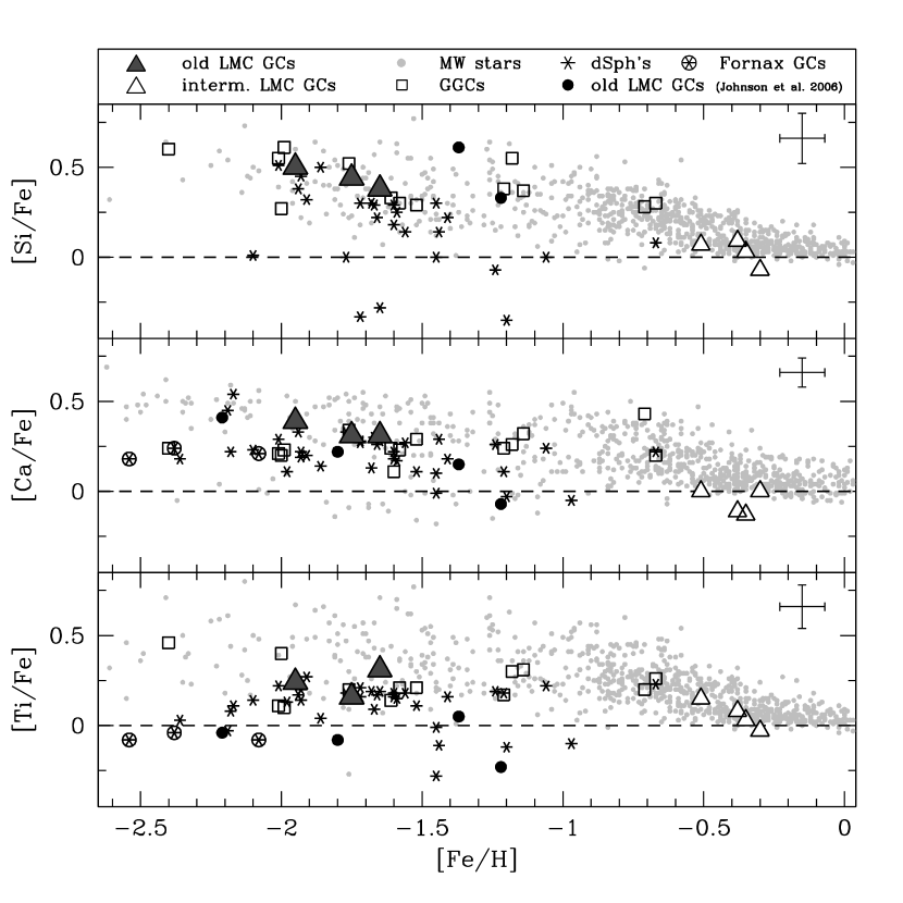
Figure 3: Behavior of [Si/Fe], [Ca/Fe] and [Ti/Fe] abundance ratios as a function of [Fe/H]. The LMC clusters of this study are plotted as grey triangles and the results by Mucciarelli et al. (2008) as white triangles. Small grey points are Galactic stars. Empty squares are GGCs. Asteriks are dSphs field stars and Fornax GCs. Black points are the old LMC GCs by Johnson et al. (2006). All the references are in Table 8. Dashed lines mark the solar value. The errorbar in the corner indicates the typical uncertainty associated to each abundance ratio and computed by summing in quadrature the internal error (reported in Tables 2-5) and the error from the adopted parameters (see Table 6).

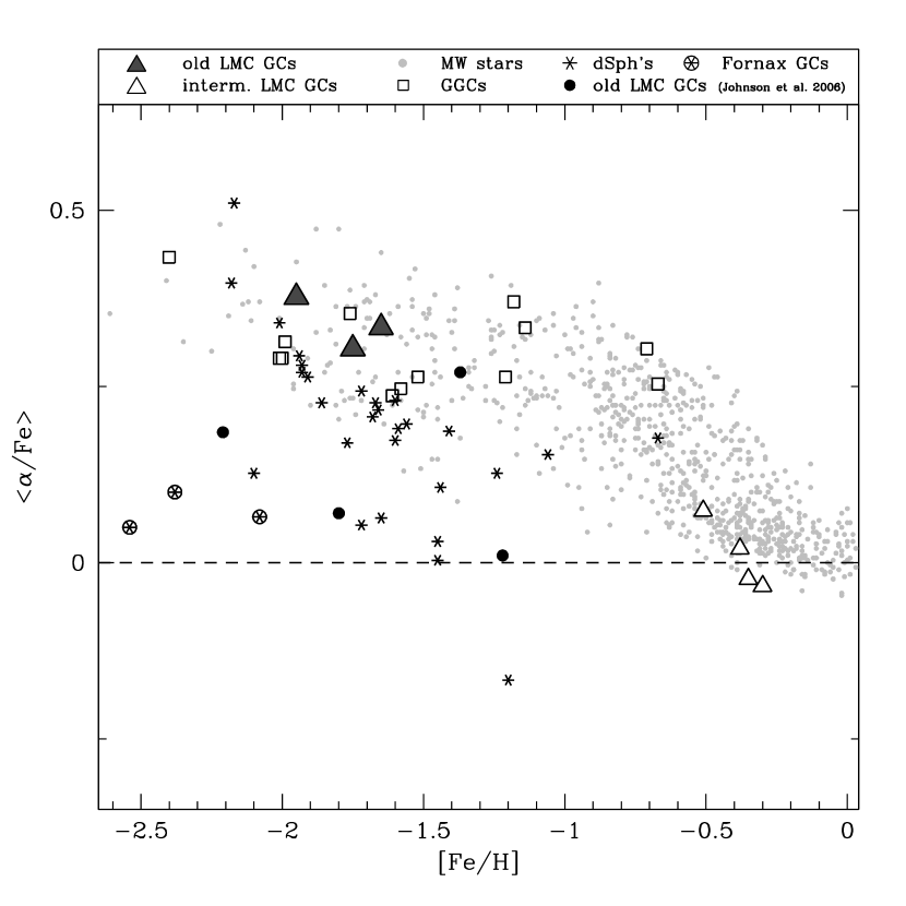
Figure 4: Behavior of the average $<\alpha/Fe>$ ratio (defined as mean of [Si/Fe], [Ca/Fe] and [Ti/Fe]) as a function of [Fe/H].

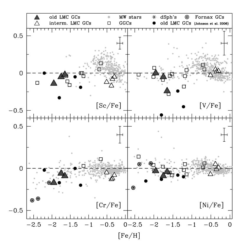
Figure 5: Behavior of [Sc/Fe], [V/Fe], [Cr/Fe] and [Ni/Fe] as a function of [Fe/H].

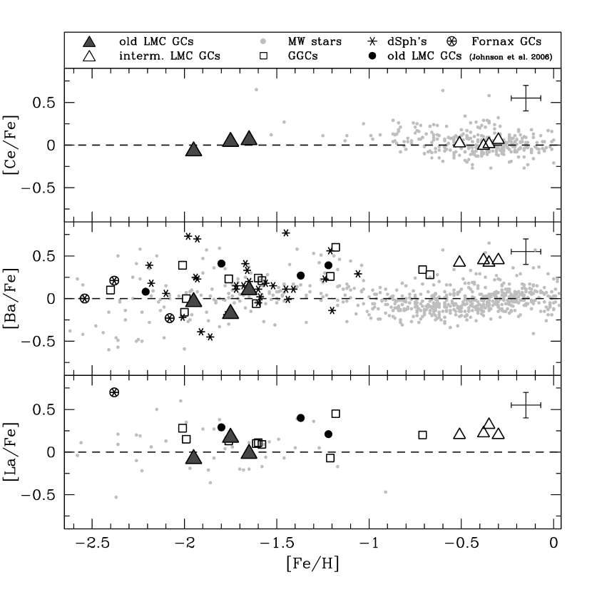
Figure 6: Behavior of [Ce/Fe], [Ba/Fe] and [La/Fe] as a function of [Fe/H].

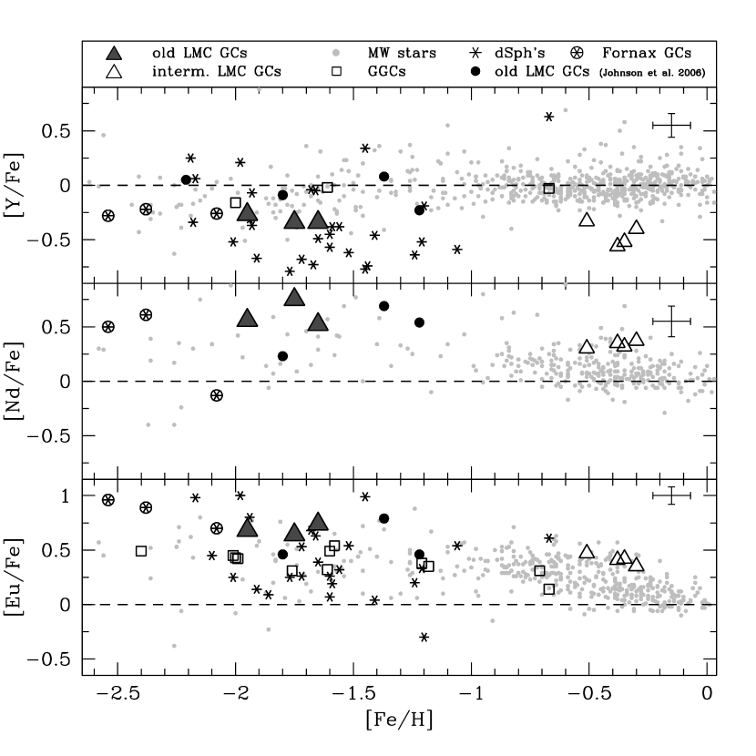
Figure 7: Behavior of [Y/Fe], [Nd/Fe] and [Eu/Fe] as a function of [Fe/H].

Tables 3 - 5 list the derived abundance ratios for all the studied stars. Table 7 summarizes the cluster average abundance ratios, together with the dispersion around the mean. Figures 3 - 7 show the plot of some abundance ratios as a function of the iron content obtained in this work (as grey triangles) and in Mucciarelli et al. (2008) (as white triangles). In these figures abundances obtained for Galactic field stars (small grey circles), GGCs (squares), dSph’s stars (asterisks) and for the sample of old LMC clusters by Johnson et al. (2006) (black points) are also plotted for comparison. All the reference sources are listed in Table 8. For sake of homogeneity and in order to avoid possible systematic effects in the comparison, we perform a study of the oscillator strengths and adopted solar values of the comparison samples, aimed at bringing all abundances in a common system. Since our analysis is differential, we decide not to correct abundances derived with the same methodology (Edvardsson et al., 1993; Gratton et al., 2003; Reddy et al., 2003, 2006). All the other dataset have been re-scaled to our adopted oscillator strengths and solar values. We compared oscillator strengths of lines in common with our list, finding, if any, negligible offsets (within $\pm$0.03 dex). Log gf of the Ti I lines adopted by Fulbright (2000), Shetrone, Coté & Sargent (2001) and Shetrone et al. (2003) are 0.07 dex higher than ours, while log gf of the Y II lines by Stephens & Boesgaard (2002) results lower than ours by -0.09 dex. The differences in the individual element solar values are small, typically less than 0.05 dex and generally the offsets of log gf and solar values cancel out, with the only exception of the Ca abundances based on the solar value by Anders & Grevesse (1989), which turns out to be 0.09 dex higher than ours.

The main abundance patterns are summarized as follows:

• Fe, O, Na, Mg and Al— Results about Fe, O, Na, Mg and Al of the target stars have been presented and discussed in Mucciarelli et al. (2009). We derived an iron content of [Fe/H]= –1.75$\pm$0.01 dex ($\sigma$= 0.02 dex),  –1.65$\pm$0.02 dex ($\sigma$= 0.04 dex) and  –1.95$\pm$0.02 dex ($\sigma$= 0.04 dex) for NGC 1786, NGC 2210 and NGC 2257, respectively.
  At variance with the other elements, Mg and Al exhibit large star-to-star variations in each cluster, while similar dishomogeneities have been found in the O content of NGC 1786 and 2257, and in the Na content of NGC 1786. Such scatters are not compatible with the observational errors and indicate the presence of intrinsic variations. The same Na-O and Mg-Al anticorrelations observed in the GGCs have been found in these LMC clusters (see Fig. 2 of Mucciarelli et al., 2009). Similar patterns have been already detected in the GGCs studied so far and they are generally interpreted in terms of a self-enrichment process, where the ejecta of the primordial Asymptotic Giant Branch (AGB) stars (in which O and Mg have been destroyed producing large amount of Na and Al) are able to trigger the formation of a second stellar generation (Ventura et al., 2001; Ventura & D’Antona, 2008). A complete discussion about the Na-O and Mg-Al anticorrelations in these 3 LMC clusters is also presented in Mucciarelli et al. (2009).

• $\alpha$-elements— Fig. 3 shows the behavior of [Si/Fe], [Ca/Fe] and [Ti/Fe] as a function of [Fe/H] for the observed clusters and the comparison samples. The first 2 abundance ratios are enhanced, with [Si/Fe]$\sim$ +0.40 dex and [Ca/Fe]$\sim$ +0.30 dex, in good agreement with the Halo and GGCs stars, while [Ti/Fe] is only moderately enhanced ($\sim$ +0.2 dex). Fig. 4 shows the average of [Si/Fe], [Ca/Fe] and [Ti/Fe] abundance ratios. We find $<\alpha/Fe>$ of 0.30$\pm$0.08, +0.33$\pm$0.02 and +0.38$\pm$0.08 for NGC 1786, 2210 and 2257, respectively. Such a level of $\alpha$-enhancement is consistent with that observed in the Galactic Halo ( both in field and cluster stars of similar metallicity), while dSphs display $<\alpha/Fe>$ ratios only $\sim$0.1-0.15 dex lower. It is worth noticing that recent studies indicate that the $\alpha$-enhancement of the Sculptor stars well agrees with the Halo stars for lower metallicities (see e.g. Tolstoy, Hill & Tosi, 2009), while the Fornax GCs show only a mild enhancement (Letarte et al., 2006), see Fig. 4.

  The only previous chemical analysis of $\alpha$-elements in old LMC GCs has been performed by Johnson et al. (2006), analyzing 4 GCs (namely, NGC 2005, 2019, 1898 and Hodge 11) in the metallicity range [Fe/H]= –2.2 / -1.2 dex (none of these objects is in common with our sample). At variance with us, they find solar or sub-solar [Ti/Fe] ratios and moderately enhanced [Ca/Fe] ratios, while their [Si/Fe] abundance ratios turn out to be enhanced in good agreement with our abundances. However, we point out that the solar zero-point for their [Ca/Fe] (including both the solar reference for Ca and Fe) is +0.11 dex higher than ours. Taking into account this offset, their Ca abundances are only 0.1 dex lower and still barely consistent within the quoted uncertainties. Conversely, for Ti, the offset in the log gf scale of -0.06 dex is not sufficient to erase the somewhat larger discrepancy ($\sim$0.2-0.3 dex) between the two abundance estimates.

• Iron-peak elements— The abundance ratios for [Sc/Fe], [V/Fe], [Cr/Fe] and [Ni/Fe] are plotted in Fig. 5. Such ratios turn out to be solar or (in a few case) moderately depleted, and consistent with the patterns observed in the Galactic Halo. The old LMC clusters analyzed by Johnson et al. (2006) exhibit similar abundance ratios, with the exception of [V/Fe] that appears to be depleted with respect to the solar value ([V/Fe]$<$–0.25 dex). V is very sensitive to the adopted $T_{eff}$, as far as Ti, and we checked possible systematic offset between our $T_{eff}$ scale and that by Johnson et al. (2006). Both scales are based on the excitational equilibrium, thus, the derived $T_{eff}$ are formally derived in a homogenous way. We checked possible offset in the adopted Fe log gf, finding an average difference $log~{}gf_{J06}$-$log~{}gf_{this~{}work}$= -0.004 ($\sigma$= 0.11). Moreover, there are no trends between the difference of the log gf and $\chi$. We repeated our analysis for some stars by using the Fe log gf by Johnson et al. (2006), finding very similar $T_{eff}$ (within $\pm$50 K) with respect to our ones. Thus, we can consider that the two $T_{eff}$ scales are compatible each other. We cannot exclude that the different treatment of the hyperfine structure for the V I lines between the two works be the origin of this discrepancy. Unfortunately, we have no GCs in common with their sample and a complete comparison cannot be performed.

• Neutron-capture elements— Elements heavier than the iron-peak (Z$>$31) are built up through rapid and slow neutron capture processes (r- and s-process, respectively). Eu is considered a pure r-process element, while the first-peak s-process element Y and the second-peak s-process elements Ba, La, Ce and Nd (see Fig. 6 and 7), have an r contribution less than $\sim$20-25% in the Sun. Nd is equally produced through s and r-process (see e.g. Arlandini et al., 1999; Burris et al., 2000). Since the s-process mainly occurs in AGB stars during the thermal pulse instability phase, s-process enriched gas should occur at later ($\sim$100-200 Myr) epochs.

  In the measured old LMC clusters we find a general depletion ($\sim$ –0.30 dex) of [Y/Fe], still consistent (within the quoted uncertainties) with the lower envelope of the [Y/Fe] distribution of the Galactic stars, which show a solar-scaled pattern. Also the metal-rich LMC clusters by Mucciarelli et al. (2008) are characterized by such a depletion, with [Y/Fe] between –0.32 and –0.54 dex (see Fig. 7). Depleted [Y/Fe] ratios have been already observed in dSphs field stars (Shetrone, Coté & Sargent, 2001; Shetrone et al., 2003) and in the Fornax GCs (Letarte et al., 2006).

  The stars of NGC 2210 and NGC 2257 exhibit roughly solar [Ba/Fe] ratios (+0.10 and –0.04 dex, respectively), while in NGC 1786 this abundance ratio is depleted ([Ba/Fe]= –0.18 dex). Also [La/Fe] and [Ce/Fe] show solar or slightly enhanced values, while [Nd/Fe] is always enhanced ($\sim$+0.50 dex). The [Ba/Fe] ratio (as far as the abundances of other heavy s-process elements) appears to be indistinguishable from the metal-poor stars in our Galaxy.

  Fig. 7 (lower panel) shows the behavior of [Eu/Fe] as a function of the [Fe/H]. The 3 old LMC clusters exhibit enhanced ($\sim$ +0.7 dex) [Eu/Fe] ratios. These values are consistent with the more Eu-rich field stars in the Galactic Halo (that display a relevant star-to-star dispersion probably due to an inhomogeneous mixing), while the GGCs are concentrated around [Eu/Fe]$\sim$+0.40 dex (James et al., 2004). The only other estimates of the [Eu/Fe] abundance ratio in LMC clusters have been provided by Johnson et al. (2006) who find enhanced values between $\sim$ +0.5 and +1.3 dex, fully consistent with our finding.

6 Discussion

The $\alpha$-elements are produced mainly in the massive stars (and ejected via type II Supernovae (SNe) explosions) during both hydrostatic and explosive nucleosynthesis. As showed in Fig. 3 and 4, the LMC clusters of our sample display a behavior of [$\alpha$/Fe] as a function of [Fe/H] similar to the one observed in the Milky Way stars. The enhanced [$\alpha$/Fe] ratios in the old LMC clusters suggest that the gas from which these objects have been formed has been enriched by type II SNe ejecta on a relative short time-scale. Such an observed pattern in the metal-poor regime agrees with the $\alpha$-enhancement of the Halo and GGCs stars, pointing out that the chemical contribution played by massive stars (concerning the nucleosynthesis of the $\alpha$-elements) in the early epochs of the LMC and Milky Way has been similar.

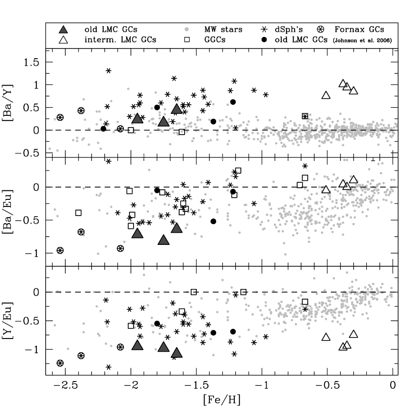
Figure 8: Behavior of [Ba/Y], [Ba/Eu] and [Y/Eu] (lower panel) as a function of [Fe/H].

[Ba/Y] is a convenient abundance ratio to estimate the relative contribution between heavy and light s-elements, [Ba/Eu] the relative contribution between heavy s and r-elements and [Y/Fe] the contribution between light s and r-elements. As shown in Fig. 8 (upper panel), [Ba/Y] is solar or moderate enhanced in old LMC as in the Milky Way, but lower than the dSphs. At higher metallicities the ratio increases appreciably due to the combined increase of Ba and decrease of Y. Such an increase of [Ba/Y] with iron content can be ascribed to the rise of the AGB contribution, with a significant metallicity dependence of the AGB yields (as pointed out by Venn et al., 2004).

In the old LMC clusters, both the [Ba/Eu] and [Y/Eu] are depleted with respect to the solar value, with [Ba/Eu]$\sim$–0.70 dex and [Y/Eu]$\sim$–1 dex. Such a depletion is consistent with the theoretical prediction by Burris et al. (2000) and Arlandini et al. (1999) in the case of pure r-process. Moreover, [Y/Eu] remains constant at all metallicities, at variance with [Ba/Eu] ratio. It is worth noticing that the precise nucleosynthesis site for Y is still unclear. Despite of the fact that most of the s-process elements are produced mainly in the He burning shell of intermediate-mass AGB stars, the lighter s-process elements, such as Y, are suspected to be synthesized also during the central He burning phase of massive stars (see e.g. the theoretical models proposed by Prantzos, Hashimoto & Nomoto, 1990). Our results suggest that in the early ages of the LMC the nucleosynthesis of the heavy elements has been dominated by the r-process, both because this type of process seems to be very efficient in the LMC and because the AGB stars have had no time to evolve and leave their chemical signatures in the interstellar medium. The contribution by the AGB stars arises at higher metallicity (and younger age) when the AGB ejecta are mixed and their contribution becomes dominant. This hypothesis has been suggested also by Shetrone et al. (2003) in order to explain the lower [Y/Fe] abundance ratios observed in dSph’s, pointing out a different Y nucleosynthesis for the Galaxy and the dSph’s, with a dominant contribution by type II SNe in the Galactic satellites.

Fig. 9 show the behaviour of [Y/$\alpha$], [Ba/$\alpha$] and [Eu/$\alpha$]. [Y/$\alpha$] and [Ba/$\alpha$] abundance ratios turns out to be depleted ($<$–0.30 dex) at low metallicity, with a weak increase at higher metallicity for [Y/$\alpha$], while [Ba/$\alpha$] reaches $\sim$+0.50 dex. This finding seems to confirm as Y is mainly produced by type II SNe, with a secondary contribution by low-metallicity AGB stars, at variance with Ba. In fact, in the low-metallicity AGB stars, the production of light s-process elements (as Y) is by-passed in favor to the heavy s-process elements (as Ba), because the number of seed nuclei (i.e. Fe) decrease decreasing the metallicity, while the neutron flux per nuclei seed increases. In light of the spectroscopic evidences arising from our database of LMC GCs and from the previous studies about Galactic and dSphs stars, both irregular and spheroidal environments seem to share a similar contribution from AGB stars and type II SNe (concerning the neutron capture elements) with respect to our Galaxy.

Our LMC clusters sample shows a remarkably constant [Eu/$\alpha$] ratio of about $\sim$ +0.4 dex over the entire metallicity range, pointing toward a highly efficient r-process mechanism . First hints of such an enhanced [Eu/$\alpha$] pattern have been found in some supergiant stars in the Magellanic Clouds (Hill et al., 1995, 1999), in Fornax GCs (Letarte et al., 2006) and field stars (Bruno Letarte, Ph.D. Thesis) and in a bunch of Sgr stars (Bonifacio et al., 2000; McWilliam & Smecker-Hane, 2005).

7 Conclusion

We have analyzed high-resolution spectra of 18 giants of 3 old LMC GCs, deriving abundance ratios for 13 elements, in addition to those already discussed in Mucciarelli et al. (2009) and sampling the different elemental groups, i.e. iron-peak, $\alpha$ and neutron-capture elements. The main results of our chemical analysis are summarized as follows:

• the three target clusters are metal-poor, with an iron content of [Fe/H]= –1.75$\pm$0.01 dex ($\sigma$= 0.02 dex),  –1.65$\pm$0.02 dex ($\sigma$= 0.04 dex) and  –1.95$\pm$0.02 dex ($\sigma$= 0.04 dex) for NGC 1786, NGC 2210 and NGC 2257, respectively (see Mucciarelli et al., 2009);

• all the three clusters show the same level of enhancement of the $<\alpha/Fe>$ ratio ($\sim$ +0.30 dex), consistent with a gas enriched by type II SNe, while metal-rich, younger LMC clusters exhibit solar-scaled $<\alpha/Fe>$ ratio, due to the contribution of type Ia SNe at later epochs;

• the iron-peak elements (Sc, V, Cr, Ni) follow a solar pattern (or slightly sub-solar, in some cases), according with the observed trend in our Galaxy and consistent with the canonical nucleosynthesis scenario;

• the studied clusters show a relevant ($\sim$–0.30 dex) depletion of [Y/Fe], while the other s-process elements (with the exception of Nd) display abundance ratios consistent with the Galactic distributions. [Ba/Fe] and [Ba/Y] in the old LMC GCs are lower than the values measured in the metal-rich, intermediate-age LMC GCs, because in the former the AGB stars had no time to evolve and enrich the interstellar medium;

• [Eu/Fe] is enhanced ($\sim$+0.70 dex) in all the clusters. This seems to suggest that the r-process elements production is very efficient in the LMC, being also the main channel of nucleosynthesis for the other neutron-capture elements.

In summary, the old, metal-poor stellar population of the LMC clusters closely resembles the GGCs in many chemical abundance patterns like the iron-peak, the $\alpha$ and heavy s-process elements, and concerning the presence of chemical anomalies for Na, O, Mg and Al. When compared with dSphs the LMC old stellar population shows remarkably different abundance patterns for [$\alpha$/Fe] and neutron-capture elements.

Figure 2: The behavior of the number density abundance of the neutral iron lines as a function of the expected line strength (upper panel), of the wavelength (middle panel) and of the excitational potential (lower panel). In each panel is also reported the linear best-fit (dashed lines) and the corresponding slope (with associated error) is labelled.

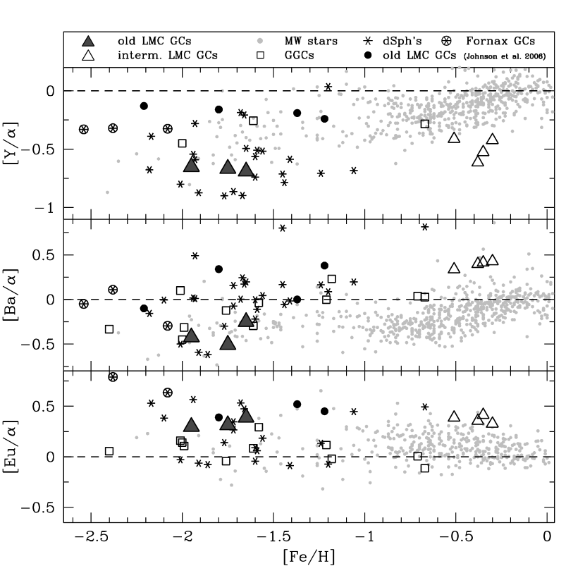
Figure 9: Behavior of [Y/$\alpha$], [Ba/$\alpha$] and [Eu/$\alpha$] as a function of [Fe/H].

Table 1: Information about the target stars. S/N have been computed at 6000 $\mathring{A}$ for the UVES spectra and at 5720 and 6260 $\mathring{A}$ for the GIRAFFE HR 11 and 13 spectra respectively. RA and Dec are onto 2MASS astrometric system. Last column reports the adopted instumental configuration (U for UVES and G for GIRAFFE spectra).

Star ID	$S/N$	$V_{helio}$	$K_{0}$	$(J-K)_{0}$	RA(J2000)	Dec(J2000)	spectrum
		(km/s)
NGC 1786-978	— / 70 / 110	260.5	13.55	0.78	74.7878641	-67.7285246	G
NGC 1786-1248	45 / — /—	255.4	13.50	0.77	74.7688292	-67.7408723	U
NGC 1786-1321	50 / — /—	273.5	13.11	0.78	74.7638489	-67.7546146	U
NGC 1786-1436	— / 60 / 90	267.1	13.71	0.72	74.7555606	-67.7353347	G
NGC 1786-1501	40 / — /—	265.9	12.92	0.93	74.7493142	-67.7514295	U
NGC 1786-2310	50 / — /—	262.2	12.83	0.82	74.7588569	-67.7432595	U
NGC 1786-2418	— / 70 / 100	265.5	13.09	0.82	74.8215213	-67.7387519	G
NGC 2210-122	40 / — /—	337.7	13.22	0.75	92.9389070	-69.1122894	U
NGC 2210-309	40 / — /—	338.4	13.29	0.75	92.9025764	-69.1129818	U
NGC 2210-431	50 / — /—	340.0	13.04	0.77	92.8887909	-69.1137252	U
NGC 2210-764	40 / — /—	335.7	12.93	0.74	92.8575073	-69.1267703	U
NGC 2210-1181	50 / — /—	335.6	12.81	0.77	92.8756190	-69.1137519	U
NGC 2257-136	40 / — /—	298.1	13.65	0.77	97.5823810	-64.3262965	U
NGC 2257-189	—  / 70 / 90	299.6	13.54	0.77	97.5741597	-64.3299382	G
NGC 2257-295	35 / — /—	301.4	14.40	0.74	97.5615868	-64.3159959	U
NGC 2257-586	—  / 50 / 60	300.6	14.36	0.70	97.5327178	-64.3129344	G
NGC 2257-842	45 / — /—	297.4	13.77	0.76	97.5591210	-64.3394905	U
NGC 2257-993	—  / 70 / 90	298.9	13.49	0.81	97.4855884	-64.3174261	G

Table 2: Atmospherical parameters and derived [Fe/H] ratio (with the number of used lines and the associated internal error defined as $\sigma/\sqrt{N_{lines}}$) for all the observed stars. Solar value for Fe is 7.54 dex (Gratton et al., 2003). Photometric temperatures (column 3) have been reported in comparison with the spectroscopic ones (column 2).

Star ID	$T_{eff}^{spec}$	$T_{eff}^{phot}$	log g	[A/H]	$v_{t}$	n	[Fe/H]
	(K)	(K)	(dex)		(km/s)		(dex)
NGC 1786-978	4250	4260	0.57	-1.75	1.40	14	-1.73 $\pm$ 0.02
NGC 1786-1248	4280	4285	0.75	-1.75	1.70	60	-1.74 $\pm$ 0.02
NGC 1786-1321	4250	4260	0.65	-1.75	1.80	54	-1.73 $\pm$ 0.01
NGC 1786-1436	4420	4412	0.76	-1.75	1.70	15	-1.76 $\pm$ 0.02
NGC 1786-1501	4100	3936	0.55	-1.80	1.80	57	-1.79 $\pm$ 0.01
NGC 1786-2310	4100	4167	0.47	-1.75	1.90	47	-1.72 $\pm$ 0.01
NGC 1786-2418	4160	4167	0.47	-1.80	1.50	16	-1.75 $\pm$ 0.02
NGC 2210-122	4300	4334	0.60	-1.65	1.70	31	-1.66 $\pm$ 0.02
NGC 2210-309	4250	4334	0.55	-1.70	1.80	35	-1.69 $\pm$ 0.03
NGC 2210-431	4200	4285	0.70	-1.65	1.80	46	-1.67 $\pm$ 0.02
NGC 2210-764	4270	4360	0.60	-1.60	1.90	42	-1.58 $\pm$ 0.02
NGC 2210-1181	4200	4285	0.60	-1.60	1.80	46	-1.64 $\pm$ 0.02
NGC 2257-136	4290	4285	0.65	-1.90	1.95	38	-1.94 $\pm$ 0.02
NGC 2257-189	4290	4285	0.61	-1.90	1.60	17	-1.92 $\pm$ 0.02
NGC 2257-295	4360	4360	0.96	-2.00	1.50	40	-1.95 $\pm$ 0.03
NGC 2257-586	4480	4466	0.82	-2.00	1.50	13	-1.92 $\pm$ 0.03
NGC 2257-842	4320	4309	0.95	-1.90	1.50	39	-1.96 $\pm$ 0.02
NGC 2257-993	4200	4190	0.52	-2.00	1.50	17	-2.02 $\pm$ 0.03

Table 3: [O/Fe], [Na/Fe], [Mg/Fe], [Al/Fe], [Si/Fe] and [Ca/Fe] abundance ratios for each observed stars with the number of used lines and the corresponding internal error.

Star ID	n	[O/Fe]	n	[Na/Fe]	n	[Mg/Fe]	n	[Al/Fe]	n	[Si/Fe]	n	[Ca/Fe]
SUN		8.79		6.21		7.43		6.23		7.53		6.27
NGC 1786-978	1	-0.15 $\pm$ 0.12	3	0.47 $\pm$ 0.03	1	0.25 $\pm$ 0.06	—	—	1	0.36$\pm$0.06	6	0.22$\pm$0.08
NGC 1786-1248	2	0.26 $\pm$ 0.08	2	0.16 $\pm$ 0.08	2	0.51 $\pm$ 0.08	—	$<$0.27	3	0.24$\pm$0.07	14	0.32$\pm$0.02
NGC 1786-1321	2	0.31 $\pm$ 0.07	2	-0.18 $\pm$ 0.07	2	0.41 $\pm$ 0.07	—	$<$0.11	3	0.49$\pm$0.06	17	0.23$\pm$0.03
NGC 1786-1436	1	0.18 $\pm$ 0.09	1	-0.01 $\pm$ 0.09	1	0.40 $\pm$ 0.09	—	—	1	0.57$\pm$0.09	5	0.37$\pm$0.07
NGC 1786-1501	2	0.30 $\pm$ 0.08	4	0.60 $\pm$ 0.06	1	0.49 $\pm$ 0.12	2	0.79 $\pm$ 0.08	1	0.41$\pm$0.12	16	0.23$\pm$0.03
NGC 1786-2310	—	$<$-0.60	3	0.66 $\pm$ 0.05	1	-0.21 $\pm$ 0.08	2	1.02 $\pm$ 0.06	4	0.51$\pm$0.04	14	0.40$\pm$0.03
NGC 1786-2418	—	$<$-0.40	4	0.77 $\pm$ 0.03	1	-0.31 $\pm$ 0.07	—	—	1	0.52$\pm$0.07	5	0.39$\pm$0.04
NGC 2210-122	2	0.31 $\pm$ 0.08	1	-0.08 $\pm$ 0.11	1	0.39 $\pm$ 0.11	—	$<$0.54	1	0.22$\pm$0.11	16	0.33$\pm$0.06
NGC 2210-309	1	0.10 $\pm$ 0.14	4	0.69 $\pm$ 0.10	1	0.20 $\pm$ 0.14	1	0.80 $\pm$ 0.14	1	0.30$\pm$0.14	15	0.49$\pm$0.05
NGC 2210-431	2	0.12 $\pm$ 0.11	3	0.64 $\pm$ 0.07	1	0.33 $\pm$ 0.12	2	0.55 $\pm$ 0.08	2	0.40$\pm$0.08	15	0.28$\pm$0.05
NGC 2210-764	2	0.25 $\pm$ 0.10	2	0.32 $\pm$ 0.10	1	0.43 $\pm$ 0.14	—	$<$0.30	2	0.48$\pm$0.10	13	0.25$\pm$0.04
NGC 2210-1181	2	0.27 $\pm$ 0.08	2	-0.03 $\pm$ 0.08	2	0.28 $\pm$ 0.11	—	$<$0.20	2	0.50$\pm$0.08	13	0.19$\pm$0.04
NGC 2257-136	1	0.22 $\pm$ 0.11	2	0.20 $\pm$ 0.11	1	0.34 $\pm$ 0.11	1	0.88 $\pm$ 0.11	2	0.54$\pm$0.08	13	0.29$\pm$0.02
NGC 2257-189	—	$<$-0.20	2	0.49 $\pm$ 0.07	1	0.42 $\pm$ 0.10	—	—	1	0.62$\pm$0.10	5	0.37$\pm$0.04
NGC 2257-295	1	0.24 $\pm$ 0.18	3	0.58 $\pm$ 0.10	1	0.12 $\pm$ 0.18	1	1.17 $\pm$ 0.18	2	0.53$\pm$0.13	14	0.53$\pm$0.03
NGC 2257-586	—	$<$-0.20	2	0.22 $\pm$ 0.08	1	0.36 $\pm$ 0.11	—	—	1	0.53$\pm$0.11	5	0.31$\pm$0.05
NGC 2257-842	1	-0.08 $\pm$ 0.15	2	0.54 $\pm$ 0.10	1	0.52 $\pm$ 0.15	—	$<$0.68	2	0.46$\pm$0.11	15	0.47$\pm$0.04
NGC 2257-993	—	$<$-0.20	2	0.90 $\pm$ 0.09	1	0.24 $\pm$ 0.13	—	—	1	0.34$\pm$0.13	5	0.39$\pm$0.04

Table 4: [Ti/Fe], [Sc/Fe] II, [V/Fe], [Cr/Fe] and [Ni/Fe] abundance ratios for each observed stars with the number of used lines and the corresponding internal error.

Star ID	n	[Ti/Fe]	n	[Sc/Fe]II	n	[V/Fe]	n	[Cr/Fe]	n	[Ni/Fe]
SUN		5.00		3.13		3.97		5.67		6.28
NGC 1786 978	3	0.11$\pm$0.03	3	-0.04$\pm$0.03	—	—	—	—	4	-0.04$\pm$0.03
NGC 1786 1248	12	0.16$\pm$0.02	5	0.06$\pm$0.07	5	0.05$\pm$0.06	5	-0.03$\pm$0.05	10	-0.12$\pm$0.02
NGC 1786 1321	9	0.13$\pm$0.02	5	-0.17$\pm$0.07	7	-0.14$\pm$0.06	6	-0.11$\pm$0.04	11	-0.08$\pm$0.04
NGC 1786 1436	4	0.40$\pm$0.05	4	-0.14$\pm$0.05	1	-0.05$\pm$0.09	—	—	2	-0.09$\pm$0.06
NGC 1786 1501	12	0.01$\pm$0.05	6	-0.05$\pm$0.06	6	-0.18$\pm$0.08	5	-0.10$\pm$0.08	10	-0.11$\pm$0.05
NGC 1786 2310	15	0.15$\pm$0.05	4	0.03$\pm$0.04	6	0.05$\pm$0.06	3	0.00$\pm$0.05	12	-0.03$\pm$0.03
NGC 1786 2418	2	0.13$\pm$0.05	4	-0.03$\pm$0.04	1	-0.04$\pm$0.07	—	—	4	-0.14$\pm$0.04
NGC 2210 122	6	0.38$\pm$0.08	5	-0.05$\pm$0.07	2	-0.23$\pm$0.08	3	-0.07$\pm$0.06	7	-0.04$\pm$0.04
NGC 2210 309	9	0.35$\pm$0.06	4	0.12$\pm$0.07	5	-0.22$\pm$0.08	3	-0.05$\pm$0.08	8	0.14$\pm$0.03
NGC 2210 431	7	0.26$\pm$0.07	5	0.06$\pm$0.04	4	-0.09$\pm$0.07	6	-0.04$\pm$0.08	7	-0.15$\pm$0.05
NGC 2210 764	7	0.26$\pm$0.09	6	-0.19$\pm$0.06	5	-0.29$\pm$0.08	3	-0.11$\pm$0.08	10	-0.01$\pm$0.07
NGC 2210 1181	5	0.28$\pm$0.09	5	-0.06$\pm$0.09	5	-0.35$\pm$0.03	3	-0.16$\pm$0.06	7	-0.14$\pm$0.08
NGC 2257 136	8	0.24$\pm$0.05	6	-0.16$\pm$0.06	1	-0.12$\pm$0.11	7	-0.06$\pm$0.07	7	0.05$\pm$0.05
NGC 2257 189	3	0.25$\pm$0.01	4	-0.19$\pm$0.05	—	—	—	—	2	0.02$\pm$0.07
NGC 2257 295	4	0.33$\pm$0.08	4	-0.10$\pm$0.08	2	0.13$\pm$0.06	4	-0.28$\pm$0.08	5	-0.11$\pm$0.04
NGC 2257 586	—	—	3	-0.17$\pm$0.06	—	—	—	—	1	-0.14$\pm$0.11
NGC 2257 842	9	0.24$\pm$0.06	6	-0.04$\pm$0.02	1	-0.01$\pm$0.15	7	-0.18$\pm$0.04	8	0.01$\pm$0.08
NGC 2257 993	3	0.16$\pm$0.05	4	-0.16$\pm$0.07	—	—	—	—	2	-0.03$\pm$0.09

Table 5: [Y/Fe] II, [Ba/Fe] II, [La/Fe] II, [Ce/Fe] II, [Nd/Fe] II and [Eu/Fe] II abundance ratios for each observed stars with the number of used lines and the corresponding internal error.

Star ID	n	[Y/Fe]II	n	[Ba/Fe]II	n	[La/Fe]II	n	[Ce/Fe]II	n	[Nd/Fe]II	n	[Eu/Fe]II
SUN		2.24		2.13		1.17		1.58		1.50		0.51
NGC 1786 978	—	—	1	-0.21$\pm$0.12	1	0.11$\pm$0.12	—	—	—	—	—	—
NGC 1786 1248	3	-0.36$\pm$0.09	3	-0.18$\pm$0.07	1	0.01$\pm$0.12	1	0.08$\pm$0.12	3	0.65$\pm$0.07	1	0.60$\pm$0.12
NGC 1786 1321	2	-0.48$\pm$0.08	3	-0.21$\pm$0.06	1	0.32$\pm$0.10	1	0.11$\pm$0.10	3	0.85$\pm$0.06	1	0.78$\pm$0.10
NGC 1786 1436	—	—	1	-0.24$\pm$0.09	—	—	—	—	—	—	—	—
NGC 1786 1501	1	-0.20$\pm$0.12	3	-0.16$\pm$0.07	1	0.24$\pm$0.12	1	-0.13$\pm$0.12	3	0.87$\pm$0.07	1	0.69$\pm$0.12
NGC 1786 2310	2	-0.32$\pm$0.06	3	-0.06$\pm$0.05	1	0.10$\pm$0.08	1	0.10$\pm$0.08	2	0.63$\pm$0.06	1	0.49$\pm$0.08
NGC 1786 2418	—	—	1	-0.19$\pm$0.07	1	0.26$\pm$0.07	—	—	—	—	—	—
NGC 2210 122	2	-0.32$\pm$0.08	3	0.11$\pm$0.06	1	-0.12$\pm$0.11	1	0.10$\pm$0.11	3	0.65$\pm$0.06	1	0.82$\pm$0.11
NGC 2210 309	1	-0.31$\pm$0.14	2	0.09$\pm$0.10	—	—	—	—	3	0.64$\pm$0.08	1	0.70$\pm$0.14
NGC 2210 431	1	-0.40$\pm$0.12	3	0.07$\pm$0.07	1	0.08$\pm$0.12	1	0.07$\pm$0.12	3	0.56$\pm$0.07	1	0.77$\pm$0.12
NGC 2210 764	2	-0.25$\pm$0.10	3	0.03$\pm$0.10	1	0.00$\pm$0.14	1	-0.08$\pm$0.14	3	0.34$\pm$0.10	1	0.75$\pm$0.14
NGC 2210 1181	2	-0.41$\pm$0.08	3	0.09$\pm$0.06	1	-0.06$\pm$0.11	1	0.15$\pm$0.11	3	0.43$\pm$0.06	1	0.63$\pm$0.11
NGC 2257 136	2	-0.29$\pm$0.08	3	0.01$\pm$0.06	1	$<$–0.10	1	$<$0.00	3	0.71$\pm$0.06	1	0.75$\pm$0.11
NGC 2257 189	—	—	1	-0.06$\pm$0.10	1	$<$–0.10	—	—	—	—	—	—
NGC 2257 295	1	-0.28$\pm$0.18	3	-0.07$\pm$0.10	1	$<$0.00	1	$<$0.10	4	0.48$\pm$0.09	1	0.59$\pm$0.18
NGC 2257 586	—	—	1	-0.11$\pm$0.11	—	—	—	—	—	—	—	—
NGC 2257 842	2	-0.23$\pm$0.11	3	-0.01$\pm$0.09	1	$<$–0.10	1	$<$0.10	3	0.50$\pm$0.09	1	0.70$\pm$0.15
NGC 2257 993	—	—	1	0.02$\pm$0.13	1	$<$–0.10	—	—	—	—	—	—

Table 6: Variation of each abundance ratio due to atmospherical parameters, obtained according to the method by Cayrel et al. (2004). Second column reports the difference for each abundance ratio between the model with $T_{eff}$ increased by 100 K (and the re-optimization of the other parameters) and the original one. The third column reports the same differences but considering a model $T_{eff}$ decreased by 100 K. The last column lists the final average error.

Ratio	$(MOD)_{+100K}$-MOD	$(MOD)_{-100K}$-MOD	Average
	(dex)	(dex)	(dex)
$[O/Fe]$	+0.13	–0.11	$\pm$0.12
$[Na/Fe]$	–0.07	+0.06	$\pm$0.07
$[Mg/Fe]$	–0.04	+0.05	$\pm$0.05
$[Al/Fe]$	–0.05	+0.04	$\pm$0.05
$[Si/Fe]$	–0.03	+0.10	$\pm$0.07
$[Ca/Fe]$	–0.02	+0.01	$\pm$0.02
$[Sc/Fe]II$	+0.06	+0.02	$\pm$0.04
$[Ti/Fe]$	+0.09	–0.10	$\pm$0.10
$[V/Fe]$	+0.11	–0.12	$\pm$0.12
$[Cr/Fe]$	+0.03	–0.06	$\pm$0.05
$[Fe/H]$	+0.08	–0.09	$\pm$0.09
$[Ni/Fe]$	+0.03	–0.02	$\pm$0.03
$[Y/Fe]II$	+0.02	–0.04	$\pm$0.04
$[Ba/Fe]II$	+0.07	–0.09	$\pm$0.09
$[La/Fe]II$	+0.15	–0.09	$\pm$0.15
$[Ce/Fe]II$	+0.09	–0.03	$\pm$0.06
$[Nd/Fe]II$	–0.08	+0.11	$\pm$0.10
$[Eu/Fe]II$	+0.04	–0.03	$\pm$0.04

Table 7: Average abundance ratios for the 3 old LMC clusters discussed in this study with the corresponding dispersion by the mean.

Ratio	NGC 1786		NGC 2210		NGC 2257
	Mean	$\sigma$	Mean	$\sigma$	Mean	$\sigma$
$[O/Fe]$	$<$–0.04	0.36	0.23	0.07	$<$–0.06	0.18
$[Na/Fe]$	0.22	0.34	0.33	0.09	0.33	0.14
$[Mg/Fe]$	0.35	0.36	0.31	0.36	0.46	0.29
$[Al/Fe]$	$<$0.55	0.43	$<$0.48	0.23	$<$0.91	0.25
$[Si/Fe]$	0.44	0.11	0.38	0.12	0.50	0.09
$[Ca/Fe]$	0.31	0.08	0.31	0.11	0.39	0.09
$[Sc/Fe]II$	–0.05	0.08	–0.02	0.12	–0.14	0.06
$[Ti/Fe]$	0.16	0.12	0.31	0.05	0.24	0.06
$[V/Fe]$	–0.05	0.09	–0.24	0.10	0.00	0.12
$[Cr/Fe]$	–0.06	0.05	–0.09	0.05	–0.17	0.11
$[Fe/H]$	–1.75	0.02	–1.65	0.04	–1.95	0.04
$[Ni/Fe]$	–0.09	0.04	–0.04	0.12	–0.03	0.08
$[Y/Fe]II$	–0.34	0.11	–0.34	0.07	–0.27	0.03
$[Ba/Fe]II$	-0.18	0.05	0.10	0.03	–0.04	0.05
$[La/Fe]II$	0.17	0.12	-0.02	0.08	$<$-0.08	0.04
$[Ce/Fe]II$	0.04	0.11	0.06	0.10	$<$-0.07	0.06
$[Nd/Fe]II$	0.75	0.12	0.52	0.14	0.56	0.13
$[Eu/Fe]II$	0.64	0.12	0.74	0.07	0.68	0.08

Note. — [Fe/H], [O/Fe], [Na/Fe], [Mg/Fe] and [Al/Fe] abundance ratios are from Mucciarelli et al. (2009) and reported here for sake of completeness.

Table 8: Literature sources for the comparison samples.

	Reference
	Galactic GCs
47 Tuc	Carretta et al. (2004), James et al. (2004)
NGC 2808	Carretta (2006)
NGC 6287	Lee & Carney (2002)
NGC 6293	Lee & Carney (2002)
NGC 6397	James et al. (2004)
NGC 6541	Lee & Carney (2002)
NGC 6752	Yong et al. (2005)
M3	Sneden et al. (2004)
M4	Ivans et al. (1999)
M5	Ivans et al. (2001)
M10	Kraft et al. (1995)
M13	Sneden et al. (2004)
M15	Sneden et al. (1997)
M71	Ramirez & Cohen. (2002)
	Galactic Field Stars
Thin/Thick	Edvardsson et al. (1993); Koch & Edvardsson (2002)
Halo	Burris et al. (2000)
Halo/Thick	Fulbright (2000)
Halo/Thick	Stephens & Boesgaard (2002)
Halo/Thick	Gratton et al. (2003)
Thin	Reddy et al. (2003)
Thick	Reddy et al. (2006)
	dSph
Draco	Shetrone, Coté & Sargent (2001)
Sextans	Shetrone, Coté & Sargent (2001)
Ursa Minor	Shetrone, Coté & Sargent (2001)
Sculptor	Shetrone et al. (2003); Geisler et al. (2005)
Fornax	Shetrone et al. (2003); Letarte et al. (2006)
Carina	Shetrone et al. (2003)
Leo I	Shetrone et al. (2003)

References

- Alonso et al. (1999) Alonso, A., Arribas, S., & Martinez-Roger, C., 1999, A&AS, 140, 261
- Alonso et al. (2001) Alonso, A., Arribas, S., & Martinez-Roger, C., 2001, A&A, 376, 1039
- Anders & Grevesse (1989) Anders, E., & Grevesse, N., 1989, Geochim. Cosmochim. Acta., 53, 197
- Andersen (1999) Andersen, J., 1999, IAU Trans. A, Vol. XXIV, (San Francisco, CA:ASP), pp. 36, 24, A36
- Arlandini et al. (1999) Arlandini, C., Kapplere, F., Wisshak, K., Gallino, R., Lugaro, M., Busso, M. & Straniero, O., 1999, ApJ, 525, 886
- Asplund (2005) Asplund, M., 2005, ARA&A, 43, 481
- Bagnulo et al. (2003) Bagnulo, S. et al.. 2003, Messenger, 114, 10
- Biemont et al. (1982) Biemont, E., Karner, C., Meyer, G., Traeger, F., & zu Putlitz, G. 1982, A&A, 107, 166
- Bonifacio et al. (2000) Bonifacio, P., Hill, V., Molaro, P., Pasquini, L., Di Marcantonio, P., & Santin, P., 2000, A&A, 359, 663
- Burris et al. (2000) Burris, D. L., Pilachowski, C. A., Armandroff, T. E., Sneden, C., Cowan, J. J., & Roe, H., 2000, ApJ, 544, 302
- Cariulo, Degl’Innocenti & Castellani (2004) Cariulo, P., Degl’Innocenti, S., & Castellani, V., 2004, A&A, 421, 1121
- Carpenter (2001) Carpenter, J. M., 2001, AJ, 121, 2851
- Carretta et al. (2004) Carretta, E., Gratton, R. G., Bragaglia, A., Bonifacio, P., & Pasquini, L., 2004. A&A, 416, 925
- Carretta (2006) Carretta, E., 2006, AJ, 131, 1766
- Cayrel (1988) Cayrel, R., 1988, in IAU Symp. 132, ”The Impact of Very High S/N Spectroscopy on Stellar Physics”, ed. G. Cayrel de Strobel & M. Spite, Dordrecht, Kluwer, 345
- Cayrel et al. (2004) Cayrel, R. et al., 2004, A&A, 416, 1117
- Dubath, Meylan & Mayor (1997) Dubath, P., Meylan, G., & Mayor, M., 1997, A&A, 324, 505
- Edvardsson et al. (1993) Edvardson, B., Andersen, J., Gustafsson, B., Lambert, L., Nissen, P. E., & Tomkin, J., 1993, A&A, 275, 101
- Ferraro et al. (2006) Ferraro, F. R., Mucciarelli, A., Carretta, E., & Origlia, L., 2006, ApJ, 645L, 33
- Fulbright (2000) Fulbright, J. P., 2000, AJ, 120, 1841
- Geisler et al. (2005) Geisler, D., Smith, V. V., Wallerstein, G., Gonzalez, G., & Charbonnel, C., 2005, AJ, 129, 1428
- Geisler et al. (2007) Geisler, D., Wallerstein, G., Smith, V. V., & Casetti-Dinescu, D. I., 2007, PASP, 119, 939
- Gopka & Yushchenko (1984) Gopka, V. F. & Yushchenko, A. V., 1984, AstL, 20, 352
- Gratton et al. (1999) Gratton, R. G., Carretta, E., Eriksson, K., & Gustafsson, B., 1999, A&A, 350, 955
- Gratton et al. (2001) Gratton, R. G. et al., 2001, A&A, 369, 87
- Gratton et al. (2003) Gratton, R. G., Carretta, E., Claudi, R., Lucatello, S., & Barbieri, M., 2003, A&A, 404, 187
- Gratton et al. (2007) Gratton, R. G., et al., 2007, A&A, 464, 953
- Grevesse & Sauval (1998) Grevesse, N, & Sauval, A. J., 1998, SSRv, 85, 161
- Grocholski et al. (2006) Grocholski, A. J., Cole, A. A., Sarajedini, A., Geisler, D., & Smith, V. V., 2006, AJ, 132, 1630
- Harris & Zaritsky (2009) Harris, J., & Zaritsky, D., 2009, AJ, 138, 1243
- Hill et al. (1995) Hill, V., Andrievsky, S., & Spite, M., 1995, A&A, 293, 347
- Hill et al. (1999) Hill, V., 1999, A&A, 345, 430
- Hill et al. (2000) Hill, V., Francois, P., Spite, M., Primas, F. & Spite, F., 2000, A&AS, 364, 19
- Koch & Edvardsson (2002) Koch, A. & Edvardsson, B., 2002, A&A, 381, 500
- Kontizas et al. (1990) Kontizas, M., Morgan, D. H., Hatzidimitriou, D., & Kontizas, E., 1990, A&AS, 84, 527
- Korn et al. (2000) Korn, A. J., Becker, S. R., Gummersbach, C. A., & Wolf, B., 2000, A&A, 353, 655
- Korn et al. (2002) Korn, A. J., Keller, S. C., Kaufer, A., Langer, N., Przybilla, N., Stahl, O., & Wolf, B., 2002, A&A, 385, 143
- Kraft et al. (1995) Kraft, R. P., Sneden, C., Langer, G. E., Shetrone, M. D., & Bolte, M., 1995, AJ, 109, 2586
- Ivans et al. (1999) Ivans, I. I., Sneden, C., Kraft, R. P., Suntzeff, N. B., Smith, V. V., Langer, G. E., & Fulbright, J. P., 1999, AJ, 118, 1273
- Ivans et al. (2001) Ivans, I. I., Kraft, R. P., Sneden, C. Smith, G. H., Rich, R. M., & Shetrone, M., 2001, AJ, 122, 1438
- Yong et al. (2005) Yong, D., Grundahl, F., Nissen, P. E., Jensen, H. R., & Lambert, D. L., 2005, A&A, 438, 875
- James et al. (2004) James, G., Francois, P., Bonifacio, P., Carretta, E., Gratton, R. G., & Spite, F., 2004, A&A, 427, 825
- Johnson et al. (2006) Johnson, J. A., Ivans, I. I.,& Stetson, P. B., 2006,ApJ, 640, 801
- Lawler et al. (2001) Lawler, J. E., Wickliffe, M. E., den Hartog, E. A., & Sneden, C., 2001, ApJ, 563, 1075
- Lecureur et al. (2007) Lecureur, A., Hill, V., Zoccali, M., Barbuy, B., Gomez, A., Minniti, D., Ortolani, S., & Renzini, A., 2007, A&A, 465, 799
- Lee & Carney (2002) Lee, J.-W., & Carney, B. W., 2002, AJ, 124, 1511
- Letarte et al. (2006) Letarte, B., Hill, V., Jablonka, P., Tolstoy, E., Francois, P., & Meylan,G., 2006, A&A, 453, 547L
- Magain (1984) Magain, P. 1984, A&A, 134, 189
- McWilliam et al. (1995) Mc William, A., Preston, G., Sneden, C., & Searle, L., 1995, AJ, 109, 2757
- McWilliam & Smecker-Hane (2005) Mc William, A. & Smecker-Hane, T. A.(2005), ASPC, 336, 221
- Monaco et al. (2005) Monaco, L., Bellazzini, M., Bonifacio, P., Ferraro, F. R., Marconi, G., Pancino, E., Sbordone, L., & Zaggia, S., 2005, A&A, 441, 141
- Monaco et al. (2007) Monaco, L., Bellazzini, M., Bonifacio, P., Buzzoni, A., Ferraro, F. R., Marconi, G., Sbordone, L., & Zaggia, S., 2007, A&A, 464, 201
- Mucciarelli et al. (2008) Mucciarelli, A., Carretta, E., Origlia, L., & Ferraro, F. R., 2008, ApJ, 136, 375
- Mucciarelli et al. (2009) Mucciarelli, A., Origlia, L., Ferraro, F. R., & Pancino, E., 2009, ApJ, 695L, 134
- Olszewski et al. (1991) Olszewski, E. W., Schommer, R. A., Suntzeff, N. B. & Harris, H. C., 1991, AJ, 101, 515
- Osterbrock et al. (1996) Osterbrock, D. E., Fulbright, J. P., Martel, A. R., Keane, M. J., Trager, S. C., & Basri, G., 1996, PASP, 108, 277
- Pasquini et al. (2002) Pasquini, L. et al., Messenger, 110, 1
- Persson et al. (1983) Persson, S. E., Aaronson, M., Cohen, J. G., Frogel, J. A., & Matthews, K.,1983
- Peterson et al. (1993) Peterson, R., C., Dalle Ore, C. M., & Kurucz, R. L., 1993, ApJ, 404, 333
- Pompeia et al. (2008) Pompeia, L., Hill, V., Spite, M., Cole, A., Primas, F., Romaniello, M., Pasquini, L., Cioni, M-R., & Smecker Hane, T., 2008, A&A, 480, 379
- Prantzos, Hashimoto & Nomoto (1990) Prantzos, N., Hashimoto, M., & Nomoto, K., 1990, A&A, 234, 211
- Prochaska (2000) Prochaska, J. X., Naumov, S. O., Carney, B. W., McWilliam, A., & Wolfe, A., 2000, AJ, 120, 2513
- Prochaska & McWilliam (2000) Prochaska, J. X., &, McWilliam, A., 2000, ApJ, 537L, 57
- Ramirez & Cohen. (2002) Ramirez, S. V., & Cohen, J., 2002, AJ, 123, 3277
- Reddy et al. (2003) Reddy, B. E., Tomkin, J., Lambert, D. L., & Allende Prieto, C., 2003, MNRAS, 340, 304
- Reddy et al. (2006) Reddy, B. E., Lambert, D. L., & Allende Prieto, C., 2006, MNRAS, 367, 1329
- Sbordone et al. (2007) Sbordone, L., Bonifacio, P., Buonanno, R., Marconi, G., Monaco, L., & Zaggia, S., 2007, A&A, 465, 815
- Shetrone, Coté & Sargent (2001) Shetrone, M., Coté, P., & Sargent, W. L. W., 2001, ApJ, 548, 592
- Shetrone et al. (2003) Shetrone, M., Venn, K. A., Tolstoy, E., Primas, F., Hill, V., & Kaufer, A., 2003, AJ, 125, 684
- Sneden et al. (1996) Sneden, C., McWilliam, A., Preston, G. W., Cowan, J. J., Burris, D. L., & Armosky, B. J., 1996, ApJ, 467, 840
- Sneden et al. (1997) Sneden, C., Kraft, R. P., Shetrone, M. D., Smith, G. H., Langer, G. E., & Prosser, C. F., 1997, AJ, 391, 354
- Sneden et al. (2004) Sneden, C., Kraft, R. P., Guhatahakurta, P., Peterson, R. C., & Fulbright, J. P., 2004, AJ, 127, 2162
- Stephens & Boesgaard (2002) Stephens, A., & Boesgaard, A. M., 2002, AJ, 123, 1647
- Tolstoy, Hill & Tosi (2009) Tolstoy, E, Hill, V, & Tosi, M., 2009, ARA&A, 47, 371
- Venn et al. (2004) Venn, K. A., Irwin, M., Shetrone, M. D., Tout, C. A., Hill, V., & Tolstoy, E., 2004, AJ, 128, 1177
- Ventura et al. (2001) Ventura, P., D’Antona, F., Mazzitelli, I., & Gratton, R., 2001, ApJ, 550L, 65
- Ventura & D’Antona (2008) Ventura, P., & D’Antona, F., 2008, MNRAS, 385, 2034
- Wahlgren (2005) Wahlgren, G. M., 2005, Memorie della Società Astronomica Italiana Supplementi, 8, 108
- Whaling et al. (1985) Whaling, W. Hannaford, P., Lowe, R. M., Biemont, E., & Grevesse, N., 1985, A&A, 153, 109