On the gluon spectrum in the glasma

Abstract

We study the gluon distribution in nucleus-nucleus collisions in the framework of the Color-Glass-Condensate. Approximate analytical solutions are compared to numerical solutions of the non-linear Yang-Mills equations. We find that the full numerical solution can be well approximated by taking the full initial condition of the fields in Coulomb gauge and using a linearized solution for the time evolution. We also compare $k_{T}$-factorized approximations to the full solution.

I Introduction

In the Color Glass Condensate (CGC) framework (for reviews see Iancu:2003xm ; Weigert:2005us ), particle multiplicities are dominated by classical gluon dynamics. The spectra of gluons produced in the collision of two heavy nuclei at high energy is determined McLerran:1994ni ; McLerran:1994ka ; McLerran:1994vd completely by the classical glasma Lappi:2006fp gauge field $A^{\mu}$ that is the solution of the classical Yang-Mills (CYM) equations of motion:

$$[D_{\mu},F^{\mu\nu}]=J^{\nu},$$ (1)

where $D_{\mu}=\partial_{\mu}-igA_{\mu}$ is the covariant derivative and $F_{\mu\nu}=\partial_{\mu}A_{\nu}-\partial_{\nu}A_{\mu}-ig[A_{\mu},A_{\nu}]$. The current $J^{\mu}$, which must be covariantly conserved ($[D_{\mu},J^{\mu}]=0$), describes the colliding nuclei. At lowest order in the color densities of the nuclei it reads

$$J^{+}=\rho_{{}_{A}}(x^{+},\mathbf{x}_{T}),\;J^{-}=\rho_{{}_{B}}(x^{-},\mathbf{x}_{T}),\;J^{i}=0,$$ (2)

with $x^{\pm}=(t\pm z)/\sqrt{2}$. This current reflects the kinematics of two nuclei $A$ and $B$ moving in the $-z$ and $+z$ direction, respectively, at almost the speed of light. With a specific gauge choice, for instance with the light-cone gauge or the Fock-Schwinger gauge, the conserved current can be fully determined, allowing us to solve the CYM equations on the light-cone. The problem of gluon production reduces then to an initial value problem of solving the CYM equations $[D_{\mu},F^{\mu\nu}]=0$ in the forward light-cone, $x^{\pm}\geq 0$. The initial condition for the gauge field can be determined explicitly by solving the CYM near the light-cone, i.e., at proper time $\tau=\sqrt{2x^{+}x^{-}}=0^{+}$.

An often used approximation for computing gluon production in heavy ion collisions is to express the spectrum as a convolution of the unintegrated gluon distribution functions, leading to the so-called $k_{T}$-factorization, which holds exactly in the dilute “pp” (proton-proton) and the dilute-dense “pA” (proton-nucleus) limits, that is, when one or both of the color sources are weak Kharzeev:2003wz ; Blaizot:2004wu ; Gelis:2005pt ; Gelis:2006tb . In these cases the CYM equations can be linearized and solved explicitly.

In a recent work Blaizot:2008yb the spectrum of gluons has been obtained by solving the Yang-Mills equations near the light-cone and treating the evolution in time linearly. It has been shown that this procedure yields the correct “pA” spectrum after expanding the solution at first order in the weak proton sources, provided one chooses a gauge that removes the transverse pure gauge component of the fields of the nuclei when they are not interacting. In the present paper, we investigate the accuracy of this approach in the nucleus-nucleus case. More precisely, the following questions will be addressed:

• What is the role of the nonlinearities in the initial condition of the CYM calculations and in the time evolution for $\tau>0$? How well can one approximate the full solution of the nonlinear equations by one where the initial condition is treated exactly but the time evolution is assumed linear?

• How good an approximation is a $k_{T}$-factorized expression for the gluon spectrum in the glasma?

We will argue in the following that a specific gauge, namely the Fock-Schwinger gauge $A_{\tau}=0$ combined with a two dimensional transverse Coulomb gauge condition $\partial_{i}A_{i}=0$ at $\tau=0^{+}$, allows us to minimize the magnitude of the initial gauge fields and therefore to reduce the “final state interactions,” i.e., the non-linear dynamics inside the forward-light-cone. We shall then, in Sec. V, discuss the range of validity of $k_{T}$-factorization.

In order to answer the questions above, we shall compare approximate solutions with the full numerical solutions of the CYM equations, obtained using the method developed in Refs. Krasnitz:1998ns ; Krasnitz:2000gz ; Krasnitz:2001qu ; Lappi:2003bi ; Krasnitz:2003jw . As we shall discuss in Sec. II, the initial conditions for the solution are given in terms of Wilson lines that, in the CGC, are random SU(3) matrices, correlated in the transverse plane over distances of order $1/Q_{\mathrm{s}}$. For our numerical studies we shall generate these Wilson lines from an implementation of the McLerran-Venugopalan (MV) model McLerran:1994ni ; McLerran:1994ka ; McLerran:1994vd (for more detail see Refs. Lappi:2003bi ; Lappi:2007ku ; Lappi:2009xa ), where the color densities are treated as random variables with a Gaussian distribution of variance

$$\langle\rho^{a}_{{}_{A}}(x^{+},\mathbf{x}_{T})\rho^{b}_{{}_{A}}(y^{+},\mathbf{y}_{T})\rangle=\\ g^{2}\mu^{2}(x^{+})\delta^{ab}\delta(x^{+}-y^{+})\delta(\mathbf{x}_{T}-\mathbf{y}_{T}),$$ (3)

for nucleus A and similarly for nucleus B. Here, $g^{2}\mu^{2}(x^{+})$ stands for the three-dimensional (squared) color charge density. After the averaging over the color densities, the observable will be only function of the two dimensional density of (squared) color charge

$$g^{2}\mu_{{}_{A}}^{2}=\int_{-\infty}^{+\infty}\,\mathrm{d}x^{+}g^{2}\mu^{2}(x^{+}).$$ (4)

We denote the value integrated over the longitudinal coordinate $x^{\pm}$ by $\mu^{2}$ without an explicit dependence on $x^{\pm}$. The saturation scale $Q_{\mathrm{s}}$ is is proportional to (and numerically of the same order of magnitude as) $g^{2}\mu_{{}_{A}}$. The relevant values are of order $g^{2}\mu_{{}_{A}}=1-2\ \textrm{GeV}$ for RHIC and $2-3\ \textrm{GeV}$ for the LHC. Note that in the convention used here $\mu^{2}_{{}_{A}}$ is a number density of charge carriers and $g^{2}\mu_{{}_{A}}^{2}$ the squared charge density. In the saturation regime $g^{2}\mu_{{}_{A}}^{2}\sim 1/\alpha_{\mathrm{s}}$ so that the saturation scale $Q_{\mathrm{s}}\sim g^{2}\mu_{{}_{A}}$ is parametrically independent of the coupling. For a discussion of the relation between the MV model parameter $g^{2}\mu$ and the saturation scale $Q_{\mathrm{s}}$ as measured in DIS experiments we refer the reader to Refs. Lappi:2007ku ; Lappi:2009xa . We emphasize that the main purpose of this paper is not to compare directly to experimental data, but to compare different approximations for the gluon spectrum in the glasma corresponding to the same distribution of color charges (or more properly Wilson lines, as we shall see shortly). Our main results would therefore be independent of the details of the color charge density distribution, and equally valid for one that would match more closely, e.g., the solution of the JIMWLK/BK evolution equations. Note however, that although we do not attempt to choose values for the parameters of our calculation to give an accurate best estimate for RHIC or the LHC, we shall stay in the phenomenologically relevant range.

II Linearized approximation of Yang-Mills equations

In this section we describe our linearized approximation for solving the CYM equations.

We work in the the Fock-Schwinger (FS) gauge $\tau A_{\tau}\equiv x^{+}A^{-}+x^{-}A^{+}=0$. In Ref. Blaizot:2008yb the discussion was formulated in terms of the light cone (LC) gauge. Appendix C of Ref. Blaizot:2008yb shows how both gauge conditions lead to the same functional form of the spectrum in the linearized approximation, Eq. (23) of the present paper. The remaining longitudinal component of the gauge field is most naturally parametrized by the component $A^{\eta}$ orthogonal to $A_{\tau}$, namely as $A^{\pm}=\pm x^{\pm}A^{\eta}$, where $\eta=\frac{1}{2}\ln(x^{+}/x^{-})$ is the spacetime rapidity.

The initial condition for the field on the light-cone is given by Kovner:1995ts ; Kovner:1995ja

$$\left.A^{i}\right|_{\tau=0^{+}} = A_{{}_{A}}^{i}+A_{{}_{B}}^{i},$$

$$\left.A^{\eta}\right|_{\tau=0^{+}} = \frac{ig}{2}[A_{{}_{A}}^{i},A_{{}_{B}}^{i}],$$ (5)

where the LC gauge fields for the individual nuclei are given by

$$A_{{}_{A}}^{i}=-\frac{1}{ig}U^{\dagger}\partial^{i}U,\;A_{{}_{B}}^{i}=-\frac{1}{ig}V^{\dagger}\partial^{i}V.$$ (6)

The fundamental degrees of freedom characterizing the CGC wavefunctions of the individual nuclei are the Wilson lines $U(\mathbf{x}_{T})$ and $V(\mathbf{x}_{T})$,

$$U(\mathbf{x}_{T})\equiv{\cal P}_{+}\exp\left[ig\int_{-\infty}^{+\infty}\,\mathrm{d}z^{+}\frac{1}{\boldsymbol{\nabla}_{T}^{2}}\rho_{{}_{A}}(z^{+},\mathbf{x}_{T})\right],$$ (7)

and

$$V(\mathbf{x}_{T})\equiv{\cal P}_{-}\exp\left[ig\int_{-\infty}^{+\infty}\,\mathrm{d}z^{-}\frac{1}{\boldsymbol{\nabla}_{T}^{2}}\rho_{{}_{B}}(z^{-},\mathbf{x}_{T})\right],$$ (8)

where $\rho_{{}_{A}}(x^{+},\mathbf{x}_{T})$ and $\rho_{{}_{B}}(x^{-},\mathbf{x}_{T})$ are the color charge densities of the nuclei. In the numerical implementation of the MV model these Wilson lines are constructed as

$$U(\mathbf{x}_{T})=\prod_{k=1}^{N_{y}}\exp\left\{-ig\frac{1}{\boldsymbol{\nabla}_{T}^{2}}\rho_{k}^{{{}_{A}},{{}_{B}}}(\mathbf{x}_{T})\right\},$$ (9)

where the color charges are Gaussian variables with the variance

$$\left\langle\rho^{a}_{k}(\mathbf{x}_{T})\rho^{b}_{l}(\mathbf{y}_{T})\right\rangle=\delta^{ab}\delta^{kl}\delta^{2}(\mathbf{x}_{T}-\mathbf{y}_{T})\frac{g^{2}\mu^{2}}{N_{y}}.$$ (10)

The indices $k,l=1\dots N_{y}$ represent a discretization of the longitudinal direction into $N_{y}$ small steps; the continuum limit corresponding to Eqs. (7) and (8) is achieved for $N_{y}\to\infty$ at constant $g^{2}\mu$. Some kind of infrared regulator is needed in order to invert the Laplacian operator $\boldsymbol{\nabla}_{T}^{2}$. One possibility is to replace $\boldsymbol{\nabla}_{T}^{2}$ in Eq. (9) by $\boldsymbol{\nabla}_{T}^{2}+m^{2}$, with a parameter $m$ chosen so that $m\ll Q_{\mathrm{s}}$. Another possibility is to set the $\mathbf{k}_{T}=\mathbf{0}_{T}$-mode of $\rho$ to zero, i.e. to impose total color neutrality on the source. This corresponds to an infrared cutoff given by the size of the system; this is the procedure we use in what follows in the cases where we take $m=0$. As noted before, our purpose is to compare different methods to obtain the gluon spectrum from the same distribution of Wilson lines. Therefore the important comparison in this context is between different approximations for the same values of $N_{y}$, $m$ and $g^{2}\mu$. We shall not carry out a a systematic study of the dependence on these parameters separately (see Ref. Lappi:2009xa for a more detailed analysis), except for the specific case of the dependence on $N_{y}$ in Sec. IV.

Note that when the fields are boost invariant, the gauge condition $A_{\tau}=0$ leads to $\partial_{+}A^{+}+\partial_{-}A^{-}=0$. This gauge, as well as the LC-gauge, does not fix completely the gauge field, and we may exploit the remaining gauge freedom in order to simplify the calculation. Imposing the restriction that we want to stay within the Fock-Schwinger gauge $A_{\tau}=0$ forbids $\tau$-dependent gauge transformations. We also want to preserve the explicit boost invariance of the field configurations and therefore we do not want to perform $\eta$-dependent transformations. This leaves us the freedom of gauge changes that depend (in the region $\tau>0$) only on the transverse coordinates. We denote the transformed field by $\mathcal{A}$:

$$\mathcal{A}^{\mu}=\Omega A^{\mu}\,\Omega^{\dagger}-\frac{1}{ig}\Omega\partial^{\mu}\Omega^{\dagger}.$$ (11)

The initial conditions in the new gauge are

$$\left.\mathcal{A}^{\eta}\right|_{\tau=0^{+}} = \frac{ig}{2}\Omega[A_{{}_{A}}^{i},A_{{}_{B}}^{i}]\Omega^{\dagger}$$

$$\left.\mathcal{A}^{i}\right|_{\tau=0^{+}} = \Omega(A_{{}_{A}}^{i}+A_{{}_{B}}^{i})\,\Omega^{\dagger}-\frac{1}{ig}\Omega\partial^{i}\Omega^{\dagger},$$ (12)

where $A_{{}_{A}}^{i}$ and $A_{{}_{B}}^{i}$ are given by Eq. (6). As we shall see, we can choose $\Omega$ so as to reduce final state interactions and treat the evolution of the fields after the collision in a linear approximation. As recalled earlier, a motivation for this strategy is the fact that, in a suitable gauge, treating the final state dynamics to lowest order in the field gives the exact solution in the case where one of the projectile is dilute and the other one dense (the “pA” case).

We shall return to the determination of $\Omega$ later, and first review the linearized solution, following Ref. Blaizot:2008yb . The linearized equations of motion, for $\tau>0$, are

$$\square\mathcal{A}^{i} = -\partial^{i}\partial^{j}\mathcal{A}^{j},$$ (13)

$$\square\mathcal{A}^{\pm} = -\partial^{\pm}\!\partial^{j}\mathcal{A}^{j}.$$ (14)

These are to be solved with the initial conditions given in Eq. (12). The second equation (14), combined with the gauge condition and boost invariance, leads to

$$\square\left[\partial^{+}\mathcal{A}^{-}+\partial^{-}\mathcal{A}^{+}\right]=2\partial^{+}\partial^{-}\partial^{j}\mathcal{A}^{j}=0,$$ (15)

which states that the divergence of the transverse field is conserved. This allows us to rewrite the Yang-Mills equations in a form that makes the boundary conditions explicit. Following the same steps as in Ref. Blaizot:2008yb , we obtain

$$\square\mathcal{A}^{i} = 2\delta(x^{+})\delta(x^{-})\left.\mathcal{A}^{i}\right|_{\tau=0^{+}}$$

$$-\theta(x^{+})\theta(x^{-})\partial^{i}\partial^{j}\left.\mathcal{A}^{j}\right|_{\tau=0^{+}},$$

$$\square\mathcal{A}^{+} = \delta(x^{-})\theta(x^{+})\left.\mathcal{A}^{\eta}\right|_{\tau=0^{+}},$$ (17)

$$\square\mathcal{A}^{-} = -\delta(x^{+})\theta(x^{-})\left.\mathcal{A}^{\eta}\right|_{\tau=0^{+}}.$$ (18)

Fourier transforming these equations we get

$$-k^{2}\mathcal{A}^{i}(k)=2\left(\delta^{ij}-\frac{k^{i}k^{j}}{2k^{+}k^{-}}\right)\left.\mathcal{A}^{j}(\mathbf{k}_{T})\right|_{\tau=0^{+}},$$ (19)

$$-k^{2}\mathcal{A}^{+}(k)=-\frac{i}{k^{-}}\left.\mathcal{A}^{\eta}(\mathbf{k}_{T})\right|_{\tau=0^{+}},$$ (20)

$$-k^{2}\mathcal{A}^{-}(k)=\frac{i}{k^{+}}\left.\mathcal{A}^{\eta}(\mathbf{k}_{T})\right|_{\tau=0^{+}}.$$ (21)

The gluon spectrum is then computed with the help of the reduction formula:

$$4\pi^{3}E\frac{\,\mathrm{d}N}{\,\mathrm{d}^{3}{\bf k}}=\sum_{\lambda}|{\cal M}_{\lambda}|^{2},$$ (22)

with the production amplitude ${\cal M}_{\lambda}=\lim\limits_{k^{2}\rightarrow 0}k^{2}\epsilon^{\lambda}_{\mu}\mathcal{A}^{\mu}(k)$ for a gluon of polarization $\lambda$. By using the completeness relation $\sum\limits_{\lambda}\epsilon_{\mu}^{\lambda}(\epsilon_{\nu}^{\lambda})^{*}=-g_{\mu\nu}$, one finally gets Blaizot:2008yb :

$$\frac{\,\mathrm{d}N}{\,\mathrm{d}y\,\mathrm{d}^{2}\mathbf{k}_{T}}=\frac{1}{(2\pi)^{2}}\frac{1}{\pi\mathbf{k}_{T}^{2}}\Big{\langle}\left|\mathbf{k}_{T}\times{\bf\cal A}(\mathbf{k}_{T})\right|^{2}\\ +\left|\mathcal{A}^{\eta}(\mathbf{k}_{T})\right|^{2}\Big{\rangle}_{\tau=0^{+}},$$ (23)

where the cross product stands for $\mathbf{k}_{T}\times{\bf\cal A}\equiv\epsilon^{ij}k^{i}\mathcal{A}^{j}$.

Let us now return to the choice of the gauge transformation $\Omega$ in Eq. (11). The choice introduced in Ref. Blaizot:2008yb (see Appendix C of  Blaizot:2008yb for the explicit derivation) was to take either $\Omega=UV$ or $\Omega=VU$. It was shown in Ref. Blaizot:2008yb that this choice reproduces correctly both the “pA” and “Ap” limits (because the gauge is not symmetric in the two nuclei one has to study the two cases separately). In general, any choice that would gauge away the pure transverse fields of the nuclei, $A^{i}_{{{}_{A}}}$ and $A^{i}_{{{}_{B}}}$, before the collision, leads to the correct answer for “pA”. Thus we look for $\Omega$ that verify the following boundary conditions: when $x^{-}<0$, i.e., in the absence of nucleus B, $\Omega\equiv U$ and when $x^{+}<0$, i.e., in the absence of nucleus A, $\Omega\equiv V$.

With the explicit expression $\Omega=VU$ one can directly perform the gauge rotations of the initial conditions in Eq. (12) to get

$$\left.\mathcal{A}^{i}\right|_{\tau=0^{+}} = V\left(UA_{{}_{B}}^{i}U^{\dagger}-A_{{}_{B}}^{i}\right)V^{\dagger}$$ (24)

$$\left.\mathcal{A}^{\eta}\right|_{\tau=0^{+}} = V\left(\partial^{i}UA_{{}_{B}}^{i}U^{\dagger}+UA_{{}_{B}}^{i}\partial^{i}U^{\dagger}\right)V^{\dagger}.$$ (25)

The expression for the spectrum that results from inserting Eqs. (24) and (25) in Eq. (23) was obtained in Ref. Blaizot:2008yb .

We now look for a gauge where the linearized evolution for $\tau>0$ works best, that is, we look for a gauge that minimizes the value of the gauge potential $\mathcal{A}$. With our restriction of boost invariance and the Fock-Schwinger condition $A_{\tau}=0$ a natural way to do this is to minimize the transverse components of $\mathcal{A}$. They are the ones in which the large unphysical pure gauge contributions show up, as can be explicitly seen in the computation of Refs. Kovner:1995ts ; Dumitru:2001ux . A convenient prescription for this is to minimize the functional $\int\,\mathrm{d}^{2}\mathbf{x}_{T}|\mathbf{A}_{T}(\mathbf{x}_{T},\tau=0^{+})|^{2}$; this is achieved by the 2-dimensional Coulomb gauge $\partial^{i}\mathcal{A}^{i}=0$. The Coulomb gauge condition is conserved by the linearized equations of motion (see Eq. (15)), so it is equivalent to impose it at $\tau=0^{+}$ or at a larger $\tau$. The full equations of motion, on the other hand, do not conserve the gauge condition. Thus in the numerical computation the gauge condition is imposed at the end of the evolution, when the gluon spectrum is calculated.

In order to impose the condition $\partial^{i}A^{i}=0$ we must then find the gauge transformation $\Omega$ as a solution of the equation

$$\partial^{i}\left(\Omega(A_{{}_{A}}^{i}+A_{{}_{B}}^{i})\,\Omega^{\dagger}-\frac{1}{ig}\Omega\partial^{i}\Omega^{\dagger}\right)=0.$$ (26)

When $x^{-}<0$, $\Omega\equiv U$ and when $x^{+}<0$, $\Omega\equiv V$ as required to reproduce the “pA” spectrum. In this case the pure transverse initial fields get rotated leading to pure longitudinal fields, i.e.,

$$\mathcal{A}^{+}=\frac{1}{\boldsymbol{\nabla}_{T}^{2}}\rho_{{}_{B}}(x^{-},\mathbf{x}_{T}),\;\mathcal{A}^{-}=\mathcal{A}^{i}=0,\;\text{for}\;x^{+}<0,$$

$$\mathcal{A}^{-}=\frac{1}{\boldsymbol{\nabla}_{T}^{2}}\rho_{{}_{A}}(x^{+},\mathbf{x}_{T}),\;\mathcal{A}^{+}=\mathcal{A}^{i}=0,\;\text{for}\;x^{-}<0.$$

In the strong field case we are not able to solve Eq. (26) for $\Omega$ analytically (or even to show formally that a unique solution exists). Finding the required gauge transformation numerically is, however, not excessively difficult and has been a standard part of the numerical CYM computations of the gluon multiplicity Krasnitz:2001qu ; Krasnitz:2000gz ; Lappi:2003bi . Indeed evaluating the approximate formula Eq. (23) in the Coulomb gauge defined by Eq. (26) is significantly less demanding than solving the full time-dependence of the Yang-Mills equations.

In the following sections we shall compare the approximate analytic solution Eq. (23) in the two gauges discussed above, $\Omega=VU$, and the Coulomb gauge choice, to the full numerical solution of the Yang-Mills equations. In addition to giving physical insight into the (admittedly gauge dependent) question of the importance of initial (meaning $\tau=0$) and final ($\tau\sim 1/Q_{\mathrm{s}}$ in this context) state interactions in the glasma this may also constitute a starting point for further analytical studies.

III Linear and nonlinear final state dynamics

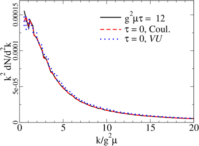
Figure 1: $\Omega=VU$ gauge gauge and Coulomb gauge results compared to the full CYM result in the weak field regime with $g^{2}\mu=0.2\ \textrm{GeV}$, $m=0.1\ \textrm{GeV}$, $N_{y}=20$. The legend “$\tau=0$” refers to the spectrum being evaluated using Eq. (23) which expresses the multiplicity in terms of the fields at $\tau=0$. The full CYM result is evaluated at $\tau=12/g^{2}\mu$.

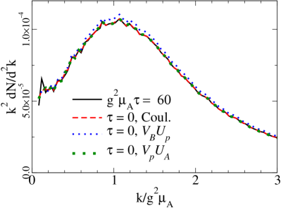
Figure 2: $\Omega=VU$ gauge and Coulomb gauge results compared to the full CYM result in the “pA” case $g^{2}\mu_{{}_{A}}=1.25\ \textrm{GeV}$, $g^{2}\mu_{p}=0.008\ \textrm{GeV}$. There are two $\Omega=VU$ gauge curves, corresponding to the cases where either the source $A$ or $B$ is taken to be weak, i.e. $V_{{}_{B}}U_{p}$: source $A$ is the proton, and $V_{p}U_{{}_{A}}$: source $B$ is the proton. It can be seen that in this limit of small $g^{2}\mu_{p}$ they are equivalent, but the $V_{{}_{B}}U_{p}$ approximation approaches the dilute limit more slowly. The CYM result is evaluated at $\tau=60/g^{2}\mu_{{}_{A}}$. $N_{y}=20$ and $m=0$.

We start by comparing the results of the linearized evolution in the $\Omega=VU$ case and the Coulomb case in the dilute limit for both sources. Figure 1 shows the gluon spectrum for $g^{2}\mu=0.2\ \textrm{GeV}$, $N_{y}=20$ and $m=0.1\ \textrm{GeV}$. This situation is dilute enough to find a good agreement; the result mainly serves as a check of the normalization in our numerical computation. The uneven structure at small $k_{T}$ in the full CYM calculation is an oscillation caused by the fact that the evolution is stopped at a finite time $\tau$; see Appendix D for a more detailed discussion.

A slightly less trivial check is provided by the “pA” case. We write this in quotation marks because what we are really computing is the dilute–dense limit where the smaller one of the two saturation scales is taken to be much smaller than the other, but also the weaker source is allowed to fill the whole transverse plane (of area $S_{\perp}=\pi R_{A}^{2}$) so that we need not worry about effects of the edge of the nucleus. Here also several analytic calculations in the Coulomb Dumitru:2001ux , covariant Kharzeev:2003wz ; Blaizot:2004wu and LC Gelis:2005pt ; Blaizot:2008yb gauges have shown that the result can be written in a $k_{T}$-factorized form, in which one needs to account for nonlinear interactions only in the initial condition. A practical question is then of course how weak the “proton” source has to be to be in this limit. Our numerical comparison is shown in Fig. 2, where the Coulomb and $\Omega=VU$ gauge approximations are seen to agree with the full numerical computation. Note that because the $\Omega=VU$ gauge prescription, Eqs. (24) and  (25), is asymmetric in the nuclei A and B, one has to look at the “pA” and “Ap” limits of the approximation separately. In Fig. 2 these are denoted by $V_{{}_{B}}U_{p}$ (source $A$ is the proton) and $V_{p}U_{{}_{A}}$ (source $B$ is the proton). Inspecting the figure closely one can see that the $V_{{}_{B}}U_{p}$ curve is slightly further away from the full CYM result. This signals the fact that the limit of nucleus $B$ being dilute converges towards the linear regime faster than the limit of $A$ being dilute, which we have verified for less asymmetric values of $g^{2}\mu_{{}_{A}}$ and $g^{2}\mu_{p}$. In other words, for the “marginal pA” case in which the proton source is weak but not infinitesimal, the gauge transformation $\Omega=V_{p}U_{{}_{A}}$ gives a slightly better approximation to the full result than $\Omega=V_{{}_{B}}U_{p}$, where the Wilson line of the proton is denoted with subscript $p$ .

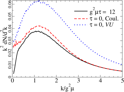
Figure 3: Light-cone gauge and Coulomb gauge results compared to the full CYM result in the saturated strong field regime with $g^{2}\mu=2\ \textrm{GeV}$, $m=0.1\ \textrm{GeV}$ $N_{y}=20$.

Let us then turn to the same comparison for the nucleus-nucleus case when both sources are strong. The comparison between the linearized prescriptions and the full result is shown in Fig. 3. We can see that the linearized Coulomb gauge result is still relatively close to the full numerical solution, but the one in $VU$-gauge starts to deviate from it significantly. After our discussion in Sec. II this behavior is easy to interpret. The Coulomb gauge condition removes, practically by construction, the unphysical pure gauge component from the field. A linearized approximation works best in a gauge that minimizes the value of the gauge potential. The $VU$-gauge condition removes the pure gauge part of the field in the “pA” case, but not in the “AA” one, because the gauge transformation required to do this is more complicated. Let us comment in more details the comparison between the linearized Coulomb gauge result with the full CYM result. We distinguish typically three regions in the spectrum:

• The high momentum range, $k_{T}/g^{2}\mu>3$. The two curves merge together, this is expected since both tend to the same limit $\sim 1/k_{T}^{2}$ at high momentum.

• The intermediate momentum region, $0.2<k_{T}/g^{2}\mu<3$ , where the two curves follow the same trend and are peaked at $k_{T}/g^{2}\mu\simeq 1.2$. In this region, our analytical formula overestimates the full CYM result by less than 15 %.

• The low momentum region, $k_{T}/g\mu^{2}<0.2$. Here, we see that the two curves diverge. The full result tends to 0 whereas our approximate formula tends to a constant.

Note that the spectrum is multiplied by $k_{T}^{2}$ in our figures, which focuses attention on the larger $k_{T}$-part and minimizes the difference between the exact calculation and the approximate ones. But the difference between the Coulomb gauge result and the full CYM result for the integrated multiplicity remains large although the spectra are close in shape. The difference in the integrated multiplicity comes mostly from the infrared part of the spectrum. Indeed since the Coulomb-gauge spectrum is logarithmically IR divergent it does not give a reliable estimate for the integrated multiplicity. One may argue that, due to the uncertainty in the CYM calculation for $k_{T}\lesssim 1/\tau$ the very small $k_{T}$-part of the spectrum in Fig. 3 is is not very reliable either. Earlier numerical studies Krasnitz:2000gz ; Krasnitz:2001qu ; Lappi:2003bi have shown, however, that the total gluon multiplicity is infrared finite. This IR-finiteness of the CYM result, presumably due to screening effects at small transverse momenta Krasnitz:2000gz ; Romatschke:2005pm ; Romatschke:2006nk , cannot be captured by a linearized treatment of the evolution for $\tau>0$.

IV Nuclear modification factor

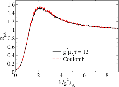
Figure 4: Nuclear modification factor of the gluon spectrum in the saturated asymmetric “pA” case $\mu_{{}_{A}}=2\ \textrm{GeV}$, $g^{2}\mu_{p}=0.32\ \textrm{GeV}$, $m=0.1\ \textrm{GeV}$ $N_{y}=500$.

We have shown in the previous section that an initial condition including all orders in the classical field in the Coulomb gauge followed by a linearized solution to the equations of motion gives a good approximation to the full solution except at very small momenta. Let us now further illustrate this point by computing the nuclear modification factors of the gluon spectrum. These are defined as the ratio of the spectrum of produced gluons to the corresponding spectrum in the dilute “pp” case, normalized by the appropriate geometrical factor, the number of binary collisions $N_{\textrm{coll}}$, to get a quantity that should approach 1 at large transverse momenta. In order to avoid complications with edge effects and Coulomb tails of the gauge field extending outside the nucleus Krasnitz:2002ng ; Krasnitz:2002mn ; Lappi:2006xc we compute the gluon spectrum in collisions of two objects of the same size (filling the whole transverse lattice), but with different saturation scales representing a proton or a nucleus. We then compare the obtained gluon spectra per unit transverse area ($S_{\perp}$) and normalize these using the expected large $k_{T}$ behavior of the gluon spectrum as $\sim(g^{2}\mu_{{}_{A}})^{2}(g^{2}\mu_{{}_{B}})^{2}/k_{T}^{4}$ to get a quantity that approaches unity at large momenta. Thus for a collision between two generic nuclei $A$ and $B$ our definition of the nuclear modification factor is

$$R_{AB}=\frac{\mu^{4}_{p}}{\mu^{2}_{{}_{A}}\mu^{2}_{{}_{B}}}\left(\frac{\,\mathrm{d}N_{AB}}{\,\mathrm{d}y\,\mathrm{d}^{2}\mathbf{k}_{T}\,\mathrm{d}^{2}S_{\perp}}\right)\left/\left(\frac{\,\mathrm{d}N_{pp}}{\,\mathrm{d}y\,\mathrm{d}^{2}\mathbf{k}_{T}\,\mathrm{d}^{2}S_{\perp}}\right)\right..$$ (28)

The experimentally measured quantity is naturally integrated over the transverse area of the collision system. In the case of a symmetric collision Eq. (28) reduces to $R_{AA}$ and for a pA collision to $R_{pA}$. In the MV model the physical interpretation of the saturation scale is straightforward as resulting from an incoherent sum of the color charges of high-$x$ partons. This leads to the scaling of the color charge density as $\mu_{{}_{A}}^{2}=A^{1/3}\mu_{p}^{2}$, and the normalization factor in $R_{AA}$ reduces to $A^{2/3}$ which is simply the number of binary collisions per unit area $\,\mathrm{d}N_{\textrm{coll}}/\,\mathrm{d}^{2}S_{\perp}$. In the proton-nucleus case the ratio of the spectra in Eq. (28) is again normalized by the number of collisions $N_{\textrm{coll}}$, which now scales like $A^{1/3}$.

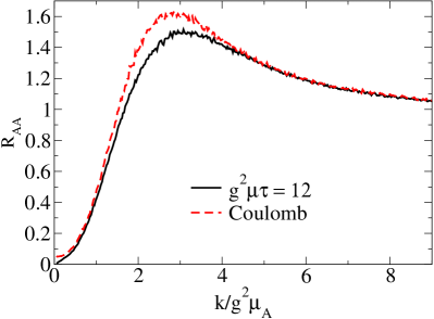
Figure 5: Nuclear modification factor $R_{AA}$, normalized with $(g^{2}\mu)^{4}$ of the gluon spectrum for $g^{2}\mu_{{}_{A}}=2\ \textrm{GeV}$, $g^{2}\mu_{p}=0.32\ \textrm{GeV}$ and $N_{y}=500$.

Our numerical results for $R_{pA}$ and $R_{AA}$ are shown in Figs. 4 and Fig. 5 respectively. They both exhibit a Cronin enhancement, peaked respectively at about two and three times the saturation scale $g^{2}\mu_{{}_{A}}$. The Cronin peak has been indeed observed in “pA” collisions, whereas in the “AA” case a large suppression of a factor 5 has been observed at RHIC, commonly understood in terms of energy loss in the hot and dense medium produced in the collision. The CYM calculation does not account for such a final sate effect.

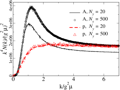
Figure 6: Scaled fundamental representation Wilson line correlators $(k_{T}^{4}/(g^{2}\mu)^{2})\mathcal{N}(\mathbf{k}_{T}/g^{2}\mu)$ for $g^{2}\mu_{{}_{A}}=2\ \textrm{GeV}$, $g^{2}\mu_{p}=0.32\ \textrm{GeV}$, $m=0.1\ \textrm{GeV}$. Results are shown for both $N_{y}=20$ and $N_{y}=500$; the latter ones are obtained from the configurations used for Figs. 4 and 5. The scaling $\mathcal{N}(\mathbf{k}_{T})\sim(g^{2}\mu)^{2}/k_{T}^{4}$ is achieved only for the larger value of $N_{y}$. When the horizontal axis is scaled with the position of the peak (i.e. $Q_{\mathrm{s}}$) instead of $g^{2}\mu$, the difference between the different values of $N_{y}$ is smaller.

There is an additional remark we must make concerning the numerical calculation. In order for the nuclear modification factor to approach one for large transverse momenta, the unintegrated gluon distribution (or Wilson line correlator $\widetilde{\mathcal{N}}(\mathbf{k}_{T})$, see Eq. (30) below) must approach the asymptotic behavior $\sim(g^{2}\mu)/\mathbf{k}_{T}^{4}$ with a constant of proportionality that is independent of any infrared scale in the problem. We have numerically found (see Ref. Lappi:2009xa for more details) that to achieve this one must discretize the longitudinal coordinate in constructing the Wilson line on a very fine grid. This means that to approach the right large $\mathbf{k}_{T}$ limit in nuclear modification factor one must use a much larger value of $N_{y}$ than was needed for the determination of $Q_{\mathrm{s}}$ in terms of $g^{2}\mu$ Lappi:2007ku or for the single or double inclusive gluon spectra in the bulk region of momenta around $Q_{\mathrm{s}}$ Lappi:2009xa . The slow convergence in the $N_{y}\to\infty$ limit is demonstrated in Fig. 6 for $\mathcal{N}$ in the fundamental representation.

As we already saw in the previous section, in the dilute-dense limit the approximation of linearized final state evolution gives the correct result. For the nuclear modification ratio $R_{pA}$ this is demonstrated in Fig. 4, where this ratio is plotted using both the full CYM result and the Coulomb gauge approximation. A slight difference between the full result and the Coulomb gauge approximation for $R_{AA}$ is seen in Fig. 5, the Coulomb gauge approximation leading to a slight overestimate.

V The $k_{T}$-factorized approximation

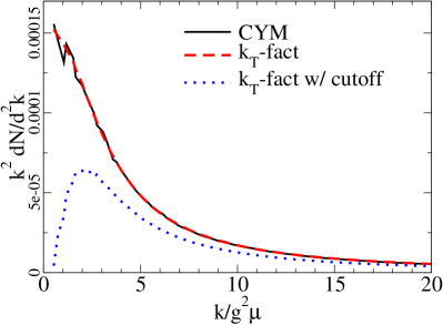
Figure 7: $k_{T}$-factorized results compared to the full CYM calculation in the dilute limit $g^{2}\mu_{{}_{A}}=0.2\ \textrm{GeV}$, $m=0.1\ \textrm{GeV}$.

As is discussed in detail in Ref. Blaizot:2008yb , there is no valid $k_{T}$-factorized expression for the gluon multiplicity in the fully nonlinear case of AA-collisions, in contrast to the case of the dilute “pA” limit. Different $k_{T}$-factorized approximations for nucleus-nucleus collisions have nevertheless been extensively used in the literature and it is therefore instructive to check how good these approximations are.

Our starting point is the following $k_{T}$-factorized ansatz for the gluon multiplicity

$$\frac{\,\mathrm{d}N}{\,\mathrm{d}y\,\mathrm{d}^{2}\mathbf{k}_{T}}=\frac{\pi R_{A}^{2}}{(2\pi)^{2}}\frac{{N_{\mathrm{c}}}^{2}-1}{2{N_{\mathrm{c}}}}\frac{2}{\pi g^{2}\mathbf{k}_{T}^{2}}\int\frac{\,\mathrm{d}^{2}\mathbf{q}_{T}}{(2\pi)^{2}}\left[\mathbf{q}_{T}^{2}\widetilde{\mathcal{N}}_{{{}_{A}}}(\mathbf{q}_{T})\right]\\ \times\left[(\mathbf{k}_{T}-\mathbf{q}_{T})^{2}\widetilde{\mathcal{N}}_{{{}_{B}}}(\mathbf{k}_{T}-\mathbf{q}_{T})\right],$$ (29)

where (for nucleus $A$)

$$\widetilde{\mathcal{N}}_{{{}_{A}}}(\mathbf{q}_{T})=\frac{1}{{N_{\mathrm{c}}}^{2}-1}\int\!\,\mathrm{d}^{2}\mathbf{r}_{T}\;e^{i\mathbf{r}_{T}\cdot\mathbf{q}_{T}}\left\langle\,\mathrm{Tr}\,\widetilde{U}^{\dagger}(\mathbf{x}_{T}+\mathbf{r}_{T})\widetilde{U}(\mathbf{x}_{T})\right\rangle$$ (30)

and similarly for $\widetilde{\mathcal{N}}_{{{}_{B}}}$ with $U$ replaced by $V$. The tilde refers to the adjoint representation, since the adjoint correlator is what appears in the A-side of the pA $k_{T}$-factorization formula. We emphasize that there is no derivation of Eq. (29) in the “AA”-case, it is an ansatz that a) is symmetric in the two nuclei and b) reduces to the correct known result in both the “pA” and the “Ap” limits, when one of the sources is taken to be weak.

The formula (29) lends itself to simplifications in different limiting cases. In particular, in the large momentum limit $|\mathbf{k}_{T}|\gg Q_{\mathrm{s}}$ the integral is dominated by the regions $\mathbf{q}_{T}\sim 0$ and $\mathbf{q}_{T}\sim\mathbf{k}_{T}$. In the first one of these regions one can approximate $\mathbf{k}_{T}-\mathbf{q}_{T}\approx\mathbf{k}_{T}$ in the second factor and pull it outside the integral; in the second region the same can be done to the other factor. This leaves the result

$$\frac{\,\mathrm{d}N}{\,\mathrm{d}y\,\mathrm{d}^{2}\mathbf{k}_{T}}=\frac{\pi R_{A}^{2}}{(2\pi)^{2}}\frac{{N_{\mathrm{c}}}^{2}-1}{2{N_{\mathrm{c}}}}\frac{2}{\pi g^{2}}\\ \left[\widetilde{\mathcal{N}}_{{}_{A}}(\mathbf{k}_{T})xG_{{}_{B}}(x,\mathbf{k}_{T}^{2})+\widetilde{\mathcal{N}}_{{}_{B}}(\mathbf{k}_{T})xG_{{}_{A}}(x,\mathbf{k}_{T}^{2})\right]$$ (31)

that is proportional to the dipole cross section or Wilson line correlation function $\widetilde{\mathcal{N}}(\mathbf{k}_{T})$ in one nucleus and the integrated gluon distribution

$$xG(x,\mathbf{k}_{T}^{2})=\int^{|\mathbf{k}_{T}|}\frac{\,\mathrm{d}^{2}\mathbf{q}_{T}}{(2\pi)^{2}}\mathbf{q}_{T}^{2}\widetilde{\mathcal{N}}(\mathbf{q}_{T})$$ (32)

in the other one. At $k_{T}\gg Q_{\mathrm{s}}$ we have parametrically $\widetilde{\mathcal{N}}(\mathbf{k}_{T})\sim Q_{\mathrm{s}}^{2}/\mathbf{k}_{T}^{4}$ (note that $\widetilde{\mathcal{N}}(\mathbf{x}_{T})$ is dimensionless) and $xG\sim Q_{\mathrm{s}}^{2}$.

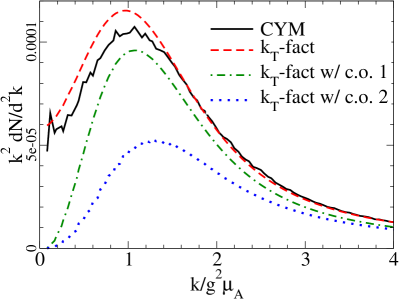
Figure 8: $k_{T}$-factorized results compared to the full CYM calculation for the “pA” case $g^{2}\mu_{{}_{A}}=1.25\ \textrm{GeV}$, $g^{2}\mu_{p}=0.008\ \textrm{GeV}$. The dot-dashed curve (“c.o. 1” i.e. “cutoff 1”) is the case where the momentum from the proton is restricted to be less than that of the produced gluon (i.e. nucleus $A$ in Eq. (29) is taken as the proton and there is a cutoff $\theta(|\mathbf{k}_{T}|-|\mathbf{q}_{T}|)$). In the dotted curve (“c.o. 2”) the cutoff is applied to the momentum from the nucleus (i.e. $B$ in Eq. (29) is the proton and the cutoff is still $\theta(|\mathbf{k}_{T}|-|\mathbf{q}_{T}|)$). The full numerical result shows a significant oscillation which is typical for a calculation at a finite ending time $g^{2}\mu_{{}_{A}}\tau=60$. $N_{y}=20$ and $m=0$.

Two main variants of the $k_{T}$-factorized formula Eq. (29) have also been used in the literature.

• The $\mathbf{q}_{T}$-integration is often cut off (see e.g. Armesto:2004ud ; Hirano:2004rs ; Drescher:2006pi ; Drescher:2006ca ; Albacete:2007sm ) with $\theta(|\mathbf{k}_{T}|-|\mathbf{q}_{T}|)$; this is asymmetric in the two nuclei but does have the advantage of making the spectrum IR-finite, which it is otherwise not. This cutoff is relatively easy to implement in our numerical evaluation, and we shall discuss its effect below.

• Instead of $\mathbf{q}_{T}^{2}\widetilde{\mathcal{N}}(\mathbf{q}_{T})$ (which we know from the pA-case to be the object appearing on the A-side) one sometimes replaces the $\mathbf{q}_{T}^{2}$ by a $1/\mathbf{r}_{T}^{2}$ inside the Fourier-transform Eq. (30). This gives an unintegrated gluon distribution $\varphi(\mathbf{q}_{T})$ (the “WW” distribution, see Kharzeev:2003wz ; Albacete:2003iq ; Blaizot:2004wu ; Gelis:2006tb ) that is related to the number of gluons as defined in LC quantization and behaves like $\ln|\mathbf{q}_{T}|$ for small momenta. This is closer to the KLN ansatz Kharzeev:2000ph ; Kharzeev:2001gp $\varphi(\mathbf{q}_{T})\sim\textrm{cst.}/\alpha_{\mathrm{s}}$. Due to the logarithmic divergence of the unintegrated gluon distribution at small $\mathbf{q}_{T}$ this approximation is more difficult to treat directly in our numerical setup and we do not study it further here.

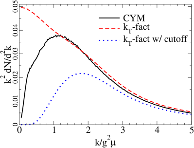
Figure 9: $k_{T}$-factorized results compared to the full CYM calculation in the saturated strong field regime, with $g^{2}\mu=2\ \textrm{GeV}$, $m=0.1\ \textrm{GeV}$ $N_{y}=20$ (same configurations as in Fig. 3).

Figure 7 shows the comparison of Eq. (29) with or without the cutoff $\theta(|\mathbf{k}_{T}|-|\mathbf{q}_{T}|)$ to the full numerical result in the dilute regime where one expects agreement. One sees that indeed, as can be shown analytically, in the dilute case the $k_{T}$-factorized expression (without the cutoff) is accurate, but the cutoff changes this already at quite high momenta. Figure 8 shows the comparison between Eq. (29) with and without the cutoff and the full result in the asymmetric “pA” case. Again we confirm the analytical calculation showing that the $k_{T}$-factorized approximation is good also in the dense-dilute case. Note the dependence on whether the momentum that is cut off is that of the proton or the nucleus. Figure 9 shows the same comparison between Eq. (29) and the full CYM result for the “AA” case. We see that while the cutoff does make the spectrum IR finite, it does so at the expense of deviating from the full result already at high momenta, $k_{T}\lesssim 2g^{2}\mu$. Unlike in the previous dilute cases, also the result without the cutoff deviates from the full result for $k_{T}\lesssim g^{2}\mu$. Comparing Figs. 9 and 3 one immediately sees that the approximation using the Coulomb gauge fields at $\tau=0$ is much more accurate than the $k_{T}$-factorized one.

Note that our result on the form of the spectrum in $k_{T}$-factorization does not invalidate computations where $k_{T}$-factorization has been used to study the dependence of the integrated multiplicity on energy, rapidity, centrality etc. The integrated multiplicity will still be, by dimensional reasons, proportional to $Q_{\mathrm{s}}^{2}$. Thus the determining aspect of these phenomenological applications is the dependence of $Q_{\mathrm{s}}$ on impact parameter and $x$, not the precise shape of the initial gluon spectrum, which will be modified later in the plasma phase.

VI Conclusion and perspectives

In conclusion, we have studied numerically the spectrum of gluons in the Glasma fields in the initial stages of a heavy ion collision. We have compared the results obtained by approximations where one includes the nonlinear interactions of the gluon fields only in the initial condition (at $\tau=0$) to the full numerical CYM calculation. The separation between initial and final state effects is not a gauge invariant one, and thus our discussion naturally involves finding a gauge that minimizes the final state effects. We find that in the Fock-Schwinger + transverse Coulomb gauge the effect of final state rescatterings on the spectrum is surprisingly small except at very small momenta. It would be interesting to see how the corrections to the linearized approximation converge towards the full CYM result.

We have also compared our results to those obtained assuming $k_{T}$-factorization. While in the “pp” and “pA” cases the results are the same, as is well known, in the fully nonlinear “AA” case $k_{T}$-factorization gives a poorer description of the gluon spectrum for $k_{T}\lesssim Q_{\mathrm{s}}$ than the linear approximation used in this paper, with a marked sensitivity to the infrared cutoff.

Appendix A Proton-Nucleus collisions and dilute limit

It was shown in Ref. Blaizot:2008yb that Eq. (23) evaluated with the $\Omega=VU$-gauge fields gives the known $k_{T}$-factorized formula for the gluon spectrum in the “pA” case. It was shown in Ref. Dumitru:2001ux that a Coulomb gauge calculation of the gluon spectrum in pA collisions gives the same result. Let us here briefly show how this comes about evaluating our Eq. (23) in Coulomb gauge. Assuming nucleus B to be a proton one can expand the gauge field to first order in $\rho_{{}_{B}}$, and we get

$$\mathcal{A}^{\eta}_{(1)}|_{\tau=0^{+}} = \frac{ig}{2}\Omega_{(0)}[A_{{{}_{A}}}^{i},A_{{{}_{B}}(1)}^{i}]\Omega^{\dagger}_{(0)}$$ (33)

$$\mathcal{A}_{(1)}^{i}|_{\tau=0^{+}} = \Omega_{(1)}A^{i}_{{}_{A}}\,\Omega^{\dagger}_{(0)}+\Omega_{(0)}A^{i}_{{}_{A}}\,\Omega^{\dagger}_{(1)}+\Omega_{(0)}A^{i}_{{{}_{B}}(1)}\,\Omega^{\dagger}_{(0)}$$

$$-\frac{1}{ig}\Omega_{(1)}\partial^{i}\Omega^{\dagger}_{(0)}-\frac{1}{ig}\Omega_{(0)}\partial^{i}\Omega^{\dagger}_{(1)},$$

where $\Omega_{(0)}\equiv U$,

$$A_{{{}_{B}}(1)}^{i}=-\frac{\partial^{i}}{\boldsymbol{\nabla}_{T}^{2}\partial^{+}}\rho_{{}_{B}},$$ (35)

and $\Omega_{(1)}$ can be extracted from Eq. (26),

$$\Omega^{\dagger}_{(1)}\equiv igU^{\dagger}\frac{\partial^{i}}{\boldsymbol{\nabla}_{T}^{2}}\left(UA^{i}_{{{}_{B}}(1)}U^{\dagger}\right).$$ (36)

We obtain after some algebra

$$\left.\mathcal{A}^{\eta}_{(1)}\right|_{\tau=0^{+}}\!\!\!\!\! = -(\partial^{i}U)A_{{{}_{B}}(1)}^{i}U^{\dagger}-UA_{{{}_{B}}(1)}^{i}(\partial^{i}U^{\dagger}),$$ (37)

$$\left.\mathcal{A}_{(1)}^{i}\right|_{\tau=0^{+}}\!\!\!\!\! = \left(\delta^{ij}-\frac{\partial^{i}\partial^{j}}{\boldsymbol{\nabla}_{T}^{2}}\right)\left(UA_{{{}_{B}}(1)}^{i}U^{\dagger}\right).$$ (38)

Plugging Eq. (37) into (23) leads to the well known $k_{T}$-factorization formula for gluon production in proton-nucleus collisions.

Appendix B Hamiltonian variables used in the numerical calculation

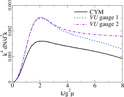
Figure 10: Different discretization methods of the VU-gauge, see text for the explanation of the labels. $g^{2}\mu=2\ \textrm{GeV}$, $N_{y}=1$ $m=0$. Note that the spectrum is multiplied by $k_{T}^{4}$ to show the effects at large $k_{T}$.

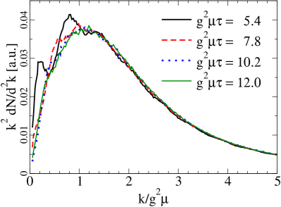
Figure 11: CYM gluon spectrum at different times. $N_{y}=20,m=0.1\ \textrm{GeV}$ (same configurations as in Fig. 3).

In the numerical calculations it is customary to work in a Hamiltonian formalism with the gauge potentials and electric fields

$$E^{i} = \tau\dot{A}_{i}$$ (39)

$$A_{\eta} = -\tau^{2}A^{\eta}=x^{+}A^{-}-x^{-}A^{+}$$ (40)

$$E^{\eta} = \frac{1}{\tau}\dot{A}_{\eta}$$ (41)

The transverse gauge potential is represented in terms of the link matrix

$$U_{i}=e^{-igaA_{i}}.$$ (42)

In Refs.Krasnitz:1998ns ; Lappi:2003bi the notation $A_{\eta}\equiv\phi$ was used, while the longitudinal electric field was denoted $E^{\eta}=\pi$ in Lappi:2003bi and $E^{\eta}=p$ in Krasnitz:1998ns . In terms of these Hamiltonian variables the initial condition Eq. (II) for the longitudinal field is

$$A_{\eta}|_{\tau=0^{+}} = 0$$ (43)

$$E^{\eta}|_{\tau=0^{+}} = -ig[A^{i}_{(1)},A^{i}_{(2)}].$$ (44)

In terms of the Hamiltonian variables the expression for the multiplicity with linearized final state evolution, Eq. (23), reads

$$\frac{\,\mathrm{d}N}{\,\mathrm{d}y\,\mathrm{d}^{2}\mathbf{k}_{T}}=\frac{1}{(2\pi)^{2}}\frac{1}{\pi\mathbf{k}_{T}^{2}}\Big{\langle}\left|\mathbf{k}_{T}\times{\bf\cal A}(\mathbf{k}_{T})\right|^{2}\\ +\left|E^{\eta}(\mathbf{k}_{T})\right|^{2}\Big{\rangle}_{\tau=0^{+}}$$ (45)

The relation between the notations in Ref. Lappi:2003bi and Ref. Blaizot:2008yb is, with Lappi:2003bi on the left and Blaizot:2008yb on the right of the equal signs, $U_{(1)}=V^{\dagger}$, $U_{(2)}=U^{\dagger}$, $A^{i}_{(1)}=-A^{i}_{{}_{B}}$ and $A^{i}_{(2)}=-A^{i}_{{}_{A}}$ (the sign is compensated by the opposite sign in the covariant derivative $\partial^{\mu}+igA^{\mu}_{(m)}=\partial^{\mu}-igA^{\mu}_{{{}_{A}},{{}_{B}}}$). Between these two references the Wilson line is exchanged with its Hermitian conjugate (including changing the direction of the path ordering in the path ordered exponential); in the conventions of Ref. Lappi:2003bi the pure gauge field is

$$A^{i}_{(1)}=-\frac{i}{g}U_{(1)}\partial^{i}U_{(1)}^{\dagger}.$$ (46)

Appendix C Discretization of Eq. (23) in the VU gauge

The formulas we need to discretize are Eq. (24):

$$\mathcal{A}^{i}=V\left(UA_{{}_{B}}U^{\dagger}-A_{{}_{B}}\right)V^{\dagger},$$ (47)

and Eq. (25)

$$\mathcal{A}^{\eta}V\left[\left(\partial^{i}U\right)A_{{}_{B}}^{i}U^{\dagger}+UA_{{}_{B}}^{i}\left(\partial^{i}U^{\dagger}\right)\right]V^{\dagger},$$ (48)

which can also be written as

$$\mathcal{A}^{\eta}=t^{a}V_{ab}\left(\partial^{i}U_{bc}\right)A_{{}_{B}}^{i,c}.$$ (49)

A straightforward way to discretize Eq. (47) is to define

$$\mathcal{A}^{i}(\mathbf{x}_{T})=\frac{1}{2}\bigg{[}V(\mathbf{x}_{T}+\mathbf{j}_{T})\Big{(}U(\mathbf{x}_{T}+\mathbf{j}_{T})A_{{}_{B}}^{j}(\mathbf{x}_{T})U^{\dagger}(\mathbf{x}_{T}+\mathbf{j}_{T})\\ -A_{{}_{B}}^{j}(\mathbf{x}_{T})\Big{)}U^{\dagger}(\mathbf{x}_{T}+\mathbf{j}_{T})\\ +V(\mathbf{x}_{T})\Big{(}U(\mathbf{x}_{T})A_{{}_{B}}^{j}(\mathbf{x}_{T})U^{\dagger}(\mathbf{x}_{T})-A_{{}_{B}}^{j}(\mathbf{x}_{T})\Big{)}V^{\dagger}(\mathbf{x}_{T})\bigg{]},$$ (50)

where $\mathbf{j}_{T}$ is a vector of length $a$ in the $j$-direction. Here the lattice gauge field is really the antihermitian part of the link matrix:

$${A_{{}_{B}}}_{i}(\mathbf{x}_{T})=-{A_{{}_{B}}}^{i}(\mathbf{x}_{T})=\frac{1}{i2ga}\left(U_{{{}_{B}},i}(\mathbf{x}_{T})-U^{\dagger}_{{{}_{B}},i}(\mathbf{x}_{T})\right),$$ (51)

where the link matrices representing the transverse pure gauge fields of the individual nuclei are

$$U^{{{}_{A}}}_{i}(\mathbf{x}_{T}) = U^{\dagger}(\mathbf{x}_{T})U(\mathbf{x}_{T}+\mathbf{i}_{T})$$ (52)

$$U^{{{}_{B}}}_{i}(\mathbf{x}_{T}) = V^{\dagger}(\mathbf{x}_{T})V(\mathbf{x}_{T}+\mathbf{i}_{T}).$$

In terms of this we then write down the discretized derivative needed in Eq. (23) as

$$\epsilon^{ij}\partial_{i}\mathcal{A}^{j}(\mathbf{x}_{T})=\epsilon^{ij}\left[\mathcal{A}^{j}(\mathbf{x}_{T}+\mathbf{i}_{T})-\mathcal{A}^{j}(\mathbf{x}_{T})\right].$$ (53)

The longitudinal field can is then discretized in the same spirit as the transverse one. The two versions Eqs. (48) and (49) lead to different-looking discretizations

$$\mathcal{A}^{\eta}=\frac{1}{2}V(\mathbf{x}_{T}+\mathbf{i}_{T})\bigg{[}U(\mathbf{x}_{T}+\mathbf{i}_{T}){A_{{}_{B}}}_{i}(\mathbf{x}_{T})U^{\dagger}(\mathbf{x}_{T}+\mathbf{i}_{T})-U(\mathbf{x}_{T}){A_{{}_{B}}}_{i}(\mathbf{x}_{T})U^{\dagger}(\mathbf{x}_{T})\bigg{]}V^{\dagger}(\mathbf{x}_{T}+\mathbf{i}_{T})\\ +\frac{1}{2}V(\mathbf{x}_{T})\bigg{[}U(\mathbf{x}_{T}+\mathbf{i}_{T}){A_{{}_{B}}}_{i}(\mathbf{x}_{T})U^{\dagger}(\mathbf{x}_{T}+\mathbf{i}_{T})-U(\mathbf{x}_{T}){A_{{}_{B}}}_{i}(\mathbf{x}_{T})U^{\dagger}(\mathbf{x}_{T})\bigg{]}V^{\dagger}(\mathbf{x}_{T})$$ (54)

and

$$\mathcal{A}^{\eta}=\frac{1}{2}V(\mathbf{x}_{T}+\mathbf{i}_{T})\bigg{[}U(\mathbf{x}_{T}+\mathbf{i}_{T}){A_{{}_{B}}}_{i}(\mathbf{x}_{T})U^{\dagger}(\mathbf{x}_{T})+U(\mathbf{x}_{T}){A_{{}_{B}}}_{i}(\mathbf{x}_{T})U^{\dagger}(\mathbf{x}_{T}+\mathbf{i}_{T})-2U(\mathbf{x}_{T}){A_{{}_{B}}}_{i}(\mathbf{x}_{T})U^{\dagger}(\mathbf{x}_{T})\bigg{]}V^{\dagger}(\mathbf{x}_{T}+\mathbf{i}_{T})\\ +\frac{1}{2}V(\mathbf{x}_{T})\bigg{[}U(\mathbf{x}_{T}+\mathbf{i}_{T}){A_{{}_{B}}}_{i}(\mathbf{x}_{T})U^{\dagger}(\mathbf{x}_{T})+U(\mathbf{x}_{T}){A_{{}_{B}}}_{i}(\mathbf{x}_{T})U^{\dagger}(\mathbf{x}_{T}+\mathbf{i}_{T})-2U(\mathbf{x}_{T}){A_{{}_{B}}}_{i}(\mathbf{x}_{T})U^{\dagger}(\mathbf{x}_{T})\bigg{]}V^{\dagger}(\mathbf{x}_{T}).$$ (55)

Of these two we prefer the first one Eq. (54) because of its relative simplicity. The combination Eqs. (50) and (54) is labeled as “$VU$-gauge 2” in Fig. 10.

An alternative discretization method is suggested by the observation that the version of the light cone gauge proposed in Blaizot:2008yb is equivalent to taking the gauge fields in the Fock-Schwinger gauge and performing a gauge rotation with the product of the Wilson lines of the two nuclei. The lattice version of initial conditions for the transverse fields is obtained Krasnitz:1998ns ; Lappi:2003bi by solving the link matrix $U_{i}(\mathbf{x}_{T})$ from the equation

$$\,\mathrm{Tr}\,\left[t_{a}\left(\left(U^{{{}_{A}}}_{i}+U^{{{}_{B}}}_{i}\right)\left(1+U_{i}^{\dagger}\right)-\mathrm{\ h.c.\ }\right)\right]=0.$$ (56)

Here the pure gauge link matrices $U_{i}^{A,B}$ (see Eq. (51)) correspond to the pure gauge fields of the two nuclei separately. For SU(2) this equation can be solved in closed form, but in the case of SU(3) that we are interested in here it is solved numerically by an iterative procedure. This link matrix $U_{i}$ is then used in the initial condition for the longitudinal field

$$E^{\eta}(\mathbf{x}_{T})=\frac{-i}{4g}\sum_{i}\bigg{[}\Big{(}U_{i}(\mathbf{x}_{T})-1\Big{)}\Big{(}U_{i}^{{\dagger}{{}_{A}}}(\mathbf{x}_{T})-U_{i}^{{\dagger}{{}_{B}}}(\mathbf{x}_{T})\Big{)}\\ +\Big{(}U_{i}^{{\dagger}}(\mathbf{x}_{T}-\mathbf{i}_{T})-1\Big{)}\Big{(}U_{i}^{{{}_{A}}}(\mathbf{x}_{T}-\mathbf{i}_{T})-U_{i}^{{{}_{B}}}(\mathbf{x}_{T}-\mathbf{i}_{T})\Big{)}-\mathrm{\ h.c.\ }\bigg{]}.$$ (57)

The fields obtained from Eqs. (56) and (57) are then gauge transformed with either $\Omega=UV$ or $\Omega=VU$ and taking the antihermitian part of the link matrix as the gauge field in Eq. (23). $VU$-gauge 1 in Fig. 10. We emphasize that the small difference between these two methods only appears at momenta of the order of the lattice UV cutoff. We observe that the UV behavior of the latter method is closer to the Coulomb gauge curve, and it is the one we use in the rest of this paper.

Appendix D Multiplicity in the CYM calculation

In the CYM computations one has to choose some finite time $\tau$ at which to perform the Fourier decomposition of the fields for computing the spectrum. In the boost invariant calculations the interactions of the fields become weaker with time, so the result does not depend very strongly on $\tau$ for $\tau\gg 1/Q_{\mathrm{s}}$. The remaining residual dependence is demonstrated in Fig. 11, which shows the resulting gluon spectrum for $g^{2}\mu\tau=4.2,7.8$ and $12$.

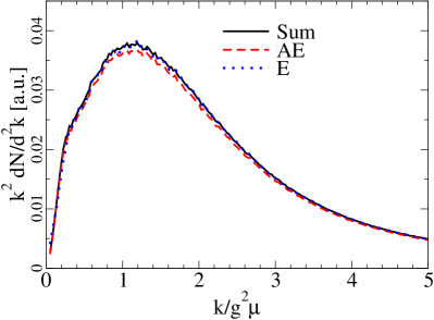
Figure 12: CYM gluon spectrum at $g^{2}\mu\tau=12$ using different methods. The solid line labeled “Sum” is the one defined by Eq. (60) that we use, unless otherwise stated, in this paper. The dashed line (“AE”) is the formula (59) that cancels the unknown dispersion relation and the dotted one (“EE”) the one of Eq. (58). $N_{y}=20,m=0.1\ \textrm{GeV}$ (the field configurations are the same as in Fig. 3).

Let us then turn to the question of defining the multiplicity corresponding to a classical field configuration that does not yet evolve completely linearly, as is the case in practical numerical computations. The straightforward method used in Lappi:2003bi is to start from the electric field part of the Hamiltonian in Coulomb gauge. The electric fields represent approximately half of the total energy of the system (which is easily verified in the full numerical computation) and because the electric field part of the Hamiltonian is quadratic in the canonical momenta one can obtain a decomposition of the total energy of the system into transverse momentum modes. If we now assume that each of these modes has a free dispersion relation $\omega(\mathbf{q}_{T})=|\mathbf{q}_{T}|$ (or the corresponding lattice equivalent in numerical computations), we get our first definition of the multiplicity

$$\frac{\,\mathrm{d}N}{\,\mathrm{d}y\,\mathrm{d}^{2}\mathbf{k}_{T}}=\frac{1}{(2\pi)^{2}}\frac{1}{|\mathbf{k}_{T}|}\Big{[}\frac{1}{\tau}E^{i}_{a}(\mathbf{k}_{T})E^{i}_{a}(-\mathbf{k}_{T})\\ +\tau\pi_{a}(\mathbf{k}_{T})\pi_{a}(-\mathbf{k}_{T})\Big{]}.$$ (58)

The dispersion relation of the interacting theory is, however, not free. The implications of this observation for our situation were observed already in the first CYM determination of the Glasma multiplicity Krasnitz:2000gz . By looking at correlators of the fields $A_{\mu}$ and the corresponding electrical fields separately one can numerically determine this dispersion relation. It was observed in Krasnitz:2000gz that this dispersion relation exhibits a mass gap that decreases with time as $m^{2}\sim g^{2}\mu/\tau$. By taking products of the correlators one can then construct a formula for the multiplicity where the dispersion relation cancels out:

$$\frac{\,\mathrm{d}N}{\,\mathrm{d}y\,\mathrm{d}^{2}\mathbf{k}_{T}}=\frac{1}{(2\pi)^{2}}\sqrt{\frac{1}{\tau}E^{i}_{a}(\mathbf{k}_{T})E^{i}_{a}(-\mathbf{k}_{T})+\tau\pi_{a}(\mathbf{k}_{T})\pi_{a}(-\mathbf{k}_{T})}\sqrt{\tau A^{i}_{a}(\mathbf{k}_{T})A^{i}_{a}(-\mathbf{k}_{T})+\frac{1}{\tau}\phi_{a}(\mathbf{k}_{T})\phi_{a}(-\mathbf{k}_{T})}.$$ (59)

The third option, and the one we will use unless otherwise stated, is based on the formal derivation from a reduction formula Gelis:2007kn . Again this is similar in spirit to our first definition and amounts to assuming a free dispersion relation $\omega(\mathbf{k}_{T})$ and taking the sum of the canonical fields and momenta as

$$\frac{\,\mathrm{d}N}{\,\mathrm{d}y\,\mathrm{d}^{2}\mathbf{k}_{T}}=\frac{1}{2(2\pi)^{2}}\bigg{\{}\frac{1}{\omega(\mathbf{k}_{T})}\bigg{[}\frac{1}{\tau}E^{i}_{a}(\mathbf{k}_{T})E^{i}_{a}(-\mathbf{k}_{T})+\tau\pi_{a}(\mathbf{k}_{T})\pi_{a}(-\mathbf{k}_{T})\bigg{]}+\omega(\mathbf{k}_{T})\bigg{[}\tau A^{i}_{a}(\mathbf{k}_{T})A^{i}_{a}(-\mathbf{k}_{T})+\frac{1}{\tau}\phi_{a}(\mathbf{k}_{T})\phi_{a}(-\mathbf{k}_{T})\bigg{]}\bigg{\}}.$$ (60)

When done properly the reduction formula also gives an additional (small in practice) contribution that is antisymmetric in $\mathbf{k}_{T}\leftrightarrow-\mathbf{k}_{T}$. This contribution vanishes when the single inclusive multiplicity is averaged over configurations and already for a single configuration when the spectrum is averaged over the azimuthal angle of $\mathbf{k}_{T}$. It is, however, important for multigluon correlations in the Glasma Gelis:2008ad ; Gelis:2008sz ; Lappi:2009xa ; Dusling:2009ni . The agreement between the three methods is illustrated in Fig. 12.

References

- (1) E. Iancu and R. Venugopalan in Quark gluon plasma (R. Hwa and X. N. Wang, eds.). World Scientific, 2003. arXiv:hep-ph/0303204.
- (2) H. Weigert, Prog. Part. Nucl. Phys. 55 (2005) 461 [arXiv:hep-ph/0501087].
- (3) L. D. McLerran and R. Venugopalan, Phys. Rev. D49 (1994) 2233 [arXiv:hep-ph/9309289].
- (4) L. D. McLerran and R. Venugopalan, Phys. Rev. D49 (1994) 3352 [arXiv:hep-ph/9311205].
- (5) L. D. McLerran and R. Venugopalan, Phys. Rev. D50 (1994) 2225 [arXiv:hep-ph/9402335].
- (6) T. Lappi and L. McLerran, Nucl. Phys. A772 (2006) 200 [arXiv:hep-ph/0602189].
- (7) D. Kharzeev, Y. V. Kovchegov and K. Tuchin, Phys. Rev. D68 (2003) 094013 [arXiv:hep-ph/0307037].
- (8) J. P. Blaizot, F. Gelis and R. Venugopalan, Nucl. Phys. A743 (2004) 13 [arXiv:hep-ph/0402256].
- (9) F. Gelis and Y. Mehtar-Tani, Phys. Rev. D73 (2006) 034019 [arXiv:hep-ph/0512079].
- (10) F. Gelis, A. M. Stasto and R. Venugopalan, Eur. Phys. J. C48 (2006) 489 [arXiv:hep-ph/0605087].
- (11) Y. V. Kovchegov, Nucl. Phys. A692 (2001) 557 [arXiv:hep-ph/0011252].
- (12) J.-P. Blaizot and Y. Mehtar-Tani, Nucl. Phys. A818 (2009) 97 [arXiv:0806.1422 [hep-ph]].
- (13) A. Krasnitz and R. Venugopalan, Nucl. Phys. B557 (1999) 237 [arXiv:hep-ph/9809433].
- (14) A. Krasnitz and R. Venugopalan, Phys. Rev. Lett. 86 (2001) 1717 [arXiv:hep-ph/0007108].
- (15) A. Krasnitz, Y. Nara and R. Venugopalan, Phys. Rev. Lett. 87 (2001) 192302 [arXiv:hep-ph/0108092].
- (16) T. Lappi, Phys. Rev. C67 (2003) 054903 [arXiv:hep-ph/0303076].
- (17) A. Krasnitz, Y. Nara and R. Venugopalan, Nucl. Phys. A727 (2003) 427 [arXiv:hep-ph/0305112].
- (18) T. Lappi, Eur. Phys. J. C55 (2008) 285 [arXiv:0711.3039 [hep-ph]].
- (19) T. Lappi, S. Srednyak and R. Venugopalan, JHEP 01 (2010) 066 [arXiv:0911.2068 [hep-ph]].
- (20) A. Kovner, L. D. McLerran and H. Weigert, Phys. Rev. D52 (1995) 3809 [arXiv:hep-ph/9505320].
- (21) A. Kovner, L. D. McLerran and H. Weigert, Phys. Rev. D52 (1995) 6231 [arXiv:hep-ph/9502289].
- (22) A. Dumitru and L. D. McLerran, Nucl. Phys. A700 (2002) 492 [arXiv:hep-ph/0105268].
- (23) P. Romatschke and R. Venugopalan, Phys. Rev. Lett. 96 (2006) 062302 [arXiv:hep-ph/0510121].
- (24) P. Romatschke and R. Venugopalan, Phys. Rev. D74 (2006) 045011 [arXiv:hep-ph/0605045].
- (25) A. Krasnitz, Y. Nara and R. Venugopalan, Phys. Lett. B554 (2003) 21 [arXiv:hep-ph/0204361].
- (26) A. Krasnitz, Y. Nara and R. Venugopalan, Nucl. Phys. A717 (2003) 268 [arXiv:hep-ph/0209269].
- (27) T. Lappi and R. Venugopalan, Phys. Rev. C74 (2006) 054905 [arXiv:nucl-th/0609021].
- (28) N. Armesto, C. A. Salgado and U. A. Wiedemann, Phys. Rev. Lett. 94 (2005) 022002 [arXiv:hep-ph/0407018].
- (29) T. Hirano and Y. Nara, Nucl. Phys. A743 (2004) 305 [arXiv:nucl-th/0404039].
- (30) H.-J. Drescher, A. Dumitru, A. Hayashigaki and Y. Nara, Phys. Rev. C74 (2006) 044905 [arXiv:nucl-th/0605012].
- (31) H. J. Drescher and Y. Nara, Phys. Rev. C75 (2007) 034905 [arXiv:nucl-th/0611017].
- (32) J. L. Albacete, Phys. Rev. Lett. 99 (2007) 262301 [arXiv:0707.2545 [hep-ph]].
- (33) J. L. Albacete, N. Armesto, A. Kovner, C. A. Salgado and U. A. Wiedemann, Phys. Rev. Lett. 92 (2004) 082001 [arXiv:hep-ph/0307179].
- (34) D. Kharzeev and M. Nardi, Phys. Lett. B507 (2001) 121 [arXiv:nucl-th/0012025].
- (35) D. Kharzeev and E. Levin, Phys. Lett. B523 (2001) 79 [arXiv:nucl-th/0108006].
- (36) F. Gelis, T. Lappi and R. Venugopalan, Int. J. Mod. Phys. E16 (2007) 2595 [arXiv:0708.0047 [hep-ph]].
- (37) F. Gelis, T. Lappi and R. Venugopalan, Phys. Rev. D78 (2008) 054020 [arXiv:0807.1306 [hep-ph]].
- (38) F. Gelis, T. Lappi and R. Venugopalan, Phys. Rev. D79 (2008) 094017 [arXiv:0810.4829 [hep-ph]].
- (39) K. Dusling, F. Gelis, T. Lappi and R. Venugopalan, Nucl. Phys. A836 (2010) 159 [arXiv:0911.2720 [hep-ph]].