Sunyaev-Zel’dovich scaling relations from a simple phenomenological model for galaxy clusters

Abstract

We build a simple, top-down model for the gas density and temperature profiles for galaxy clusters. The gas is assumed to be in hydrostatic equilibrium along with a component of non-thermal pressure taken from simulations and the gas fraction approaches the cosmic mean value only at the virial radius or beyond. The free parameters of the model are the slope and normalisation of the concentration-mass relation, the gas polytropic index, and slope and normalisation of the mass-temperature relation. These parameters can be fixed from X-Ray and lensing observations. We compare our gas pressure profiles to the recently proposed ‘Universal’ pressure profile by Arnaud et al. (2009) and find very good agreement. We find that the Sunyaev-Zel’dovich Effect (SZE) scaling relations between the integrated SZE flux, $Y$, the cluster gas temperature, $T_{\rm sl}$, the cluster mass, $M_{\rm tot}$, and the gas mass, $M_{\rm gas}$ are in excellent agreement with the recently observed $r_{2500}$ SZE scaling relations by Bonamente et al. (2008) and $r_{500}$ relation by Arnaud et al. (2009). The gas mass fraction increases with cluster mass and is given by $f_{\rm gas}(r_{500})=0.1324+0.0284\,\rm{log}\,(\frac{M_{500}}{10^{15}h^{-1}M_{\odot}})$. This is within $10\%$ of observed $f_{\rm gas}(r_{500})$. The consistency between the global properties of clusters detected in X-Rays and in SZE shows that we are looking at a common population of clusters as a whole, and there is no deficit of SZE flux relative to expectations from X-Ray scaling properties. Thus, it makes it easier to compare and cross-calibrate clusters from upcoming X-Ray and SZE surveys.

1 Introduction

Large yield SZE cluster surveys promise to do precision cosmology once cluster mass-observable scaling relations are reliably calibrated. This can be done through cluster observations (Benson et al., 2004; Bonamente et al., 2008), simulations (da Silva et al., 2004; Bonaldi et al., 2007) and analytic modeling (Bulbul et al., 2010). It is well known that different astrophysical processes influence the cluster mass-observable relations non-trivially (for example, see Balogh et al. (2001); Borgani et al. (2004); Kravtsov et al. (2005); Puchwein et al. (2008)) which can lead to biases in determining cosmology with clusters. Alternatively, one can ‘self-calibrate’ the uncertainties (Majumdar & Mohr, 2003, 2004; Lima & Hu, 2004).

Simplistic modeling of the intra-cluster medium (ICM), like the ‘isothermal $\beta$-model’ can give rise to inaccuracies. More complex modeling needs additional assumptions (such as gas following dark matter at large radii (Komatsu & Seljak, 2001), hereafter KS) or inclusion of less understood baryonic physics (Ostriker et al., 2005).

To partially circumvent our incomplete knowledge of cluster gas physics, we build a top-down phenomenological model of cluster structure, taking clues from both observations and simulations. It stands on three simple, well motivated, assumptions: (i) present X-Ray observations can give reliable cluster mass-temperature relations at $r<r_{500}$ which is used to calibrate our models; (ii) the gas mass fraction, $f_{\rm gas}$, increases with radius as seen in observations (Vikhlinin et al., 2006; Sun et al., 2009) and in simulations (Ettori et al., 2006), with non-gravitational processes pushing the gas outwards. It reaches values close to universal baryon fraction at or beyond the virial radius; and (iii) there is a component of non-thermal pressure support whose value relative to thermal pressure can be inferred from biases in mass estimates found in simulations (see Rasia et al. (2004)). This simple model can reproduce the ‘Universal’ pressure profile (Arnaud et al., 2009), X-Ray gas fraction, and SZE scaling relations in excellent agreement with observations.

2 The Cluster Model

2.1 The Cluster Mass Profiles

The NFW profile (Navarro et al., 1997) is typically used to describe the dark matter mass profile. Here we adopt a NFW form for the total matter profile since we use the observationally estimated concentration parameter given by Comerford & Natarajan (2007) $c_{vir}=\frac{14.5\pm 6.4}{1+z}(M_{\rm vir}/M_{\star})^{-0.15\pm 0.13}$. Here $M_{\star}=1.3\times 10^{13}h^{-1}M_{\odot}$. The virial radius, $r_{\rm vir}$, is calculated from the spherical collapse model (Peebles, 1980) as $r_{\rm vir}=\left[\frac{M_{vir}}{\frac{4\pi}{3}\rho_{crit}(z)\Delta_{c}(z)}\right]^{1/3}$. Here, $\Delta_{c}(z)=18\pi^{2}+82x-39x^{2}$ (Bryan & Norman, 1998) and $x=\Omega_{m}(z)-1$.

2.2 The Temperature and density Profiles

XMM-Newton and Chandra observations have shown that the cluster temperature declines at large radii (Arnaud et al., 2005; Vikhlinin et al., 2006) for both cool (CC) and non-cool core (NCC) clusters. Simulations (Ascasibar et al., 2003; Borgani et al., 2004), observations (Sanderson & Ponman, 2010) and analytic studies (Bulbul et al., 2010) indicate polytropic profiles for gas temperature. These studies also point towards an almost constant polytropic index $\gamma\sim 1.2$ (atleast, till $r_{500}$). Hence, we adopt $T(r)=T(0)f(r)^{\gamma-1}$ and $\rho(r)=\rho(0)f(r)$ . We take the fiducial $\gamma$ = 1.2.

We have also compared the resulting temperature profiles with recent observations (Pratt et al., 2007; Sun et al., 2009) and find the decrements to be comparable . Alternatively, for our “Best-fit” models we let the $\gamma$ vary along with the $M_{0}$ and $\alpha$ of the M-T relation and find the values that give the best-fit to the SZ Scaling relations. Further, CC clusters are characterized by central temperature decrements which we take to be $T(r)\propto r^{0.3}$ (Sanderson et al., 2006) below $0.1r_{500}$.

To calculate ICM density and temperature profiles, we use the gas dynamical equation (Binney & Tremaine, 1987; Rasia et al., 2004):

$$\frac{d\Phi(r)}{dr}\,=\,\frac{1}{\rho(r)}\frac{dP(r)}{dr}+\frac{1}{\rho(r)}\frac{d[\rho(r)\sigma_{r}^{2}(r)]}{dr}+2\beta(r)\frac{\sigma_{r}^{2}(r)}{r}\;,$$ (1)

where $\Phi$ is the gravitational potential, $\sigma_{r}^{2}(r)$ is the gas velocity dispersion, $\beta(r)$ is the velocity dispersion anisotropy parameter (put equal to zero in this work) and $P(r)$ and $\rho(r)$, the gas pressure and density where $P(r)=\frac{\rho(r)}{\mu m_{p}}kT(r)$. Here, $m_{p}$ is the proton mass and $\mu$ is the mean molecular weight. For hydrostatic equilibrium without non-thermal pressure, $\frac{d\Phi(r)}{dr}=\frac{1}{\rho(r)}\frac{dP(r)}{dr}$. This is normally used to obtain ICM profiles for a given halo (for example, in Komatsu & Seljak (2001)).

Simulations (Rasia et al., 2004; Battaglia et al., 2010) show that non-thermal pressure can be significant especially at large radii. Both observations (Mahdavi et al., 2008; Zhang et al., 2008) and simulations (Nagai et al., 2007; Lau et al., 2009) suggest that the cluster mass calculated assuming only hydrostatic equilibrium is less than the true mass of a cluster. This discrepancy increases with radius. Typical values are 20-40% at $r_{\rm vir}$. The velocity dispersion term arises from the bulk motions of the ICM and contributes to the non-thermal pressure support. The profile f(r) can thus be numerically obtained by solving equation 1.

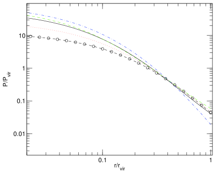
Figure 1: The normalized ICM pressure, $P/P_{vir}$ is plotted against cluster radius for a cluster of mass $5\times 10^{14}h^{-1}$ $M_{\odot}$ and z = 0. The thick black solid line is the fiducial model; the blue dot-dashed line is for $P_{non-th}=0$; the green dashed line has polytropic index changed to 1.12 from 1.2; the red dotted line is for lower concentration. The KS model pressure is given by the black solid line with circles. Note, that the SZE flux is given by the line-of-sight integral of $P(r)$ over a given cluster area.

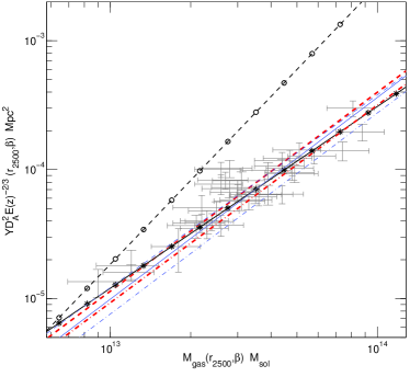
Figure 2: Left Panel: The $f_{gas}$ at $r_{500}$ is plotted against $M_{500}$ for the cluster. The topmost horizontal line is for $f_{\rm gas}=\frac{\Omega_{b}}{\Omega_{m}}$; the solid and dot-dashed lines are for KS model for two different halo concentrations; the dotted line is for our fiducial model and the dashed line is from X-Ray observations (Vikhlinin et al., 2009). Right Panel: The $Y-M_{\rm gas}$ scaling relations at $r_{2500}$ for our models are shown with the data points from Bonamente et al. (2008) and the best fit Bonamente relation.The 5 lines pertaining to our models are - (i) thin blue solid line for model 1 (fiducial), (ii)thin blue dashed line for model 2 , (iii)thin blue dot-dashed line for model 3, (iv) Thick red dot-dashed line for the model ‘Bestfit-1’ and (v) thick red dashed line for the model ‘Bestfit-3’ (see text for details). The Bonamente bestfit to data is given by the black solid line with stars. The KS model is shown by dashed line with circles.

2.2.1 Temperature and Density Normalization

The temperature profiles are normalized to the recently observed X-Ray $M_{500}-T_{\rm sp}$ scaling relation found by Sun et al. (2009) which includes data from cluster to group scales and is given by

$$M_{500}E(z)=M_{0}\left[\frac{T_{\rm sp}}{3{\rm keV}}\right]^{\alpha}$$ (2)

where $M_{0}=(1.21\pm 0.08)\times 10^{14}h^{-1}M_{\odot}$ and $\alpha=1.68\pm.04$. Here $M_{500}$ is the mass within $r_{500}$, where the average density is $500\rho_{c}(z)$ where $\rho_{c}(z)$ is the critical density at redshift z. Using the prescription given by Mazzotta et al. (2004) we estimate the ‘spectroscopic-like’ temperature $T_{\rm sl}$, a particular weighted average of $T(r)$. This value of $\alpha\neq 1.5$ indicates deviation from self-similarity, pointing to non-gravitational energetics in the ICM. Here we bypass the microphysics that breaks ‘self-similarity’ but normalize the cluster temperatures so as to exactly reproduce the observed $M-T_{\rm sl}$ relation. Thus our cluster model can be thought of as a top-down model.

For any point in parameter space, representative of a simulated cluster, we calculate analytically the temperature and density profiles. We start with an initial arbitrary T(0) and solve for f(r) as described earlier. Next, $T_{\rm sl}$, is calculated in the radial range $0.1r_{500}$ - $r_{500}$. The original T(0) is now adjusted by the ratio of $T_{\rm sl}$ to the $T_{sp}$ from the observed $M_{500}-T_{\rm sp}$ relation. The equation for $f(r)$ is now solved with this new $T(0)$ after which the $T_{\rm sl}$ is again calculated. In a few iterations, a self consistent profile f(r) is obtained. Next, $\rho(0)$ is determined by equating the $f_{gas}$ within the cluster radius to 0.9($\Omega_{b}$/$\Omega_{m}$) at the cluster boundary ($r_{200}$ or beyond). The Universal baryon fraction $\Omega_{b}$/$\Omega_{m}$ is given by 0.167 $\pm$ .009 (Komatsu et al., 2010).

Simulations (Ettori et al., 2006) and observations (Vikhlinin et al., 2006; Sun et al., 2009) show the gas mass fraction, $f_{gas}(r)=\frac{M_{\rm gas}(r)}{M_{tot}(r)}$, increases with radius. Stellar mass which accounts for a finite fraction of the baryons is larger at smaller radii such as $r_{2500}$ and for group scale haloes, as observed in the above mentioned studies. Radiative simulations tend to underestimate $f_{gas}$ due to overcooling and predict $f_{gas}=0.7-0.8(\Omega_{b}/\Omega_{m})$ at $r_{vir}$. Allowing 10% of the baryons to form stars, we take $f_{gas}=0.9(\Omega_{b}/\Omega_{m})$ at the cluster boundary. The resulting $f_{gas}$ as seen in fig 2 shows good agreement with the observations at $r_{500}$. We assume that non-gravitational effects only redistribute the gas. Recently, both observations (Rasheed et al., 2010) and theoretical studies (Battaglia et al., 2010; Nath & Majumdar, 2010) show that gas is driven outside the virial radius $r_{vir}$ and atleast upto $2r_{vir}$.

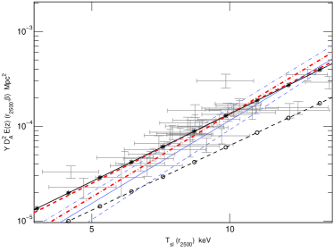
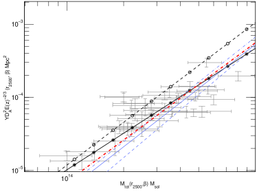
Figure 3: Left panel : The $Y-T_{\rm sl}$ relation. The lines here have the same meaning as in figure 2, except that the thick red dashed line is now for our model ‘Bestfit-2’ (see text). Right panel: The $Y-M_{\rm tot}$ relation at $r_{2500}$ is plotted. The line scheme is the same.

Table 1: SZ Scaling Relations at $r_{2500}$ : ${\rm log}(YD_{A}^{2}E(z)^{\delta})=A+B{\rm log}(X/c_{x})$ where $c_{\rm T_{sl}}=8{\rm keV},c_{\rm m_{gas}}=3*10^{13}M_{\odot}$ and $c_{\rm m{tot}}=3*10^{14}M_{\odot}$ and $(\delta=1,-2/3,-2/3)$ for $(X=T_{\rm sl},M_{\rm gas},M_{\rm tot})$.

	Y-$T_{sl}$			Y-$M_{\rm gas}$			Y-$M_{\rm tot}$
	A	B	$\Delta\chi^{2}$	A	B	$\Delta\chi^{2}$	A	B	$\Delta\chi^{2}$
Bonamente	-4.10$\pm$0.22	2.37$\pm$0.23	.0017	-4.25$\pm$1.77	1.41$\pm$0.13	.073	-4.20$\pm$3.00	1.66$\pm$0.20	.047
Best fit	-4.094	2.363		-4.25	1.414		-4.19	1.654
model1	-4.215	2.906	0.57	-4.258	1.565	0.12	-4.322	2.003	0.71
model2	-4.342	3.149	2.04	-4.201	1.495	0.024	-4.441	2.170	1.83
model3	-4.093	2.944	0 .19	-4.376	1.56	1.31	-4.245	2.047	0.24
K-S	-4.410	2.28	6.64	-3.630	2.18	11.55	-4.050	1.95	0.46
Bestfit-1	-4.153	2.909	0.20	-4.301	1.533	0.39	-4.247	1.902	0.23
Bestfit-2	-4.103	2.448	0 .0067	-	-	-	-	-	-
Bestfit-3	-	-	-	-4.207	1.544	0.038	-	-	-

2.3 Model Descriptions

We include non-thermal pressure, $P_{\rm non-th}$, in our calculations. However, this contribution to the total pressure ($P_{tot}$) for a cluster is difficult to model analytically.

In this work, we follow gas dynamical simulations by Rasia et al. (2004) to estimate the $P_{\rm non-th}$. We adopt their $P_{th}$/$P_{tot}$ as an input to our model. The mass of the cluster calculated from the hydrostatic term only is lower than the true mass by $\sim 15\%$ at $r_{500}$, $\sim 30\%$ at $r_{vir}$ and $\sim 40\%$ at $2r_{vir}$ in our fiducial model. These values when compared with figure 13 in their paper are found to be of comparable magnitude.

We consider the following models :

• model 1 (the fiducial model): Here $f_{\rm gas}=0.9(\frac{\Omega_{b}}{\Omega_{m}})$ at $r=r_{\rm vir}$ ; $M_{0}=1.728\times 10^{14}M_{\odot}$, $\alpha$ = 1.68 and $\gamma$ =1.2. We follow Rasia et al. (2004) to estimate $P_{\rm non-th}/P_{\rm total}$.

• model 2: similar to model 1 but $f_{\rm gas}=0.9(\frac{\Omega_{b}}{\Omega_{m}})$ at $r=2r_{\rm vir}$. $P_{\rm non-th}/P_{\rm total}$ is extrapolated beyond $r_{vir}$ following simulations by Rasia.

• model 3: parameters same as in model 1 but for ‘zero’ $P_{\rm non-th}$.

Other than these models, we look at variations of the fiducial model, where we vary the parameters $M_{0},\alpha\,{\rm and}\,\gamma$, to get the best fit to the Bonamente et al. (2008) SZE data. These are called Bestfit-1, Bestfit-2 and Bestfit-3 and give a minimum to $\chi^{2}_{tot}=\chi^{2}_{(Y-T_{\rm sl})}+\chi^{2}_{(Y-M_{\rm gas})}+\chi^{2}_{(Y-M_{\rm tot})}$, $\chi^{2}_{(Y-T_{\rm sl})}$, and $\chi^{2}_{(Y-M_{\rm gas})}$ respectively, where the $\chi^{2}$ is to Bonamente data.

In figure 1, we show the effect of varying some of the model parameters on the ICM pressure profile for a $5\times 10^{14}h^{-1}M_{\odot}$ cluster normalized to $P_{vir}$ which is taken to be the ICM pressure at $r_{vir}$ for the standard self-similar model (see Arnaud et al. (2009), Appendix A). Inclusion of non-thermal pressure leads to shallower slope at large radii compared to only thermal pressure. The polytropic index has little influence on the pressure profile for the given change in $\gamma$. The integrated SZE, unlike X-Ray, is similar for both CC and NCC clusters. In figure 2 (left panel), we show that clusters in our model naturally have a mass dependent gas fraction, in agreement with observed $f_{\rm gas}$ to within 10% for $M_{500}\raisebox{-1.29167pt}{\mbox{$\stackrel{{\scriptstyle>}}{{{}_{\sim}}}\,$}}2\times 10^{14}h^{-1}M_{\odot}$. For our fiducial model, we find :
$f_{\rm gas}(r_{500})=0.1324+0.0284$ $\rm{log}(\frac{M_{500}}{10^{15}h^{-1}M_{\odot}})$.

3 The SZE scaling relations - observations and and theoretical models

The measurement of SZE (Sunyaev & Zeldovich, 1980) has come of age in recent times with improvement in detector technologies. Both targeted observations (say from OVRO/BIMA/SZA) and blank sky surveys (ACT/SPT) are underway having much cosmological potential (Carlstrom et al., 2002). Targeted observations have recently given us the SZE scaling relations which can now be used in surveys as proxy for mass.

The SZE scaling relations (Bonamente et al., 2008) predicted from self-similar theory are :

$$YD_{A}^{2} \propto f_{gas}T_{\rm sl}^{5/2}E(z)^{-1}$$

$$YD_{A}^{2} \propto f_{gas}M_{\rm tot}^{5/3}E(z)^{2/3}$$

$$YD_{A}^{2} \propto f_{gas}^{-2/3}M_{\rm gas}^{5/3}E(z)^{2/3}$$ (3)

where $Y$ is the the integrated SZE flux from the cluster, $D_{A}$ is the angular diameter distance. $M_{\rm gas}$ and $M_{\rm tot}$ are the gas mass and total mass.

3.1 The $r_{2500}$ Scaling Relations

Benson et al. (2004) presented the first observed SZE scaling relations between the central decrement, $y_{0},Y$ and $T_{\rm sl}$ for a sample of 14 clusters. Recently, Bonamente et al. (2008) have published scaling relations for 38 clusters at $0.14\leq z\leq 0.89$ using Chandra X-Ray observations and radio observations with BIMA / OVRO. Weak lensing mass measurements, at $r_{4000-8000}$, of SZE clusters have now been done by Marrone et al. (2009) to give the $Y-M_{\rm tot}$ scaling. Their extrapolated masses at $r_{2500}$ show agreement to within $20\%$ to the hydrostatic mass estimates by Bonamente et al. (2008). We follow Bonamente et al. (2008) in constructing our scaling relations. In particular we fit beta profiles to the density profile as well as the x-ray surface brightness $S_{X}$ and compton y parameter obtained by projecting the temperature and density profiles obtained as a result of solving equation 1. :

$$y=\frac{k_{B}\sigma_{T}}{m_{e}c^{2}}\int Tn_{e}\,dl;\hskip 56.9055ptS_{X} \propto \int n_{e}^{2}\,dl$$ (4)

The isothermal temperature for each cluster is calculated in the same radial annulus as theirs. The SZE flux is found by integrating the SZE $\beta$-profiles and the total mass assuming hydrostatic equilibrium is estimated using $M_{\rm tot}(r)=\frac{3\beta k_{B}T_{\rm sl}r^{3}}{G\mu m_{p}(r_{c}^{2}+r^{2})}$. With this prescription, we construct the three power law scaling relations given in equation 3. The coefficients for these scaling relations are specified in table 1. For comparison, we also calculate the SZE scaling relations from $\beta$-fits to the often used ‘Komatsu-Seljak’ (KS) model (Komatsu & Seljak, 2001). A comparison of the SZE scaling relation for our models, the KS model and the Bonamente data are shown in figures 2 and 3 and table 1.

The first point to notice is the good agreement of our model scaling relations with the Bonamente best fit. Especially, for the $Y-M_{\rm gas}$ relation, our models are in excellent agreement with observations. This is relevant as observationally the $Y-M_{\rm gas}$ relation has the least uncertainty. However the assumption of a $\beta$-model for the ICM adds to the uncertainty. For the $Y-T_{\rm sl}$ relation, our estimate of $T_{\rm sl}$ is not accurate for lower temperatures and the agreement with the Bonamente data becomes worse. Especially, for lower $T_{\rm sl}$, our models under predict the SZE flux. Note, that for both of these relations, the KS model line lies outside the data points and hence is a very bad fit to SZE scalings. Our models also under predicts the SZE flux for masses below $M_{2500}\sim 3\times 10^{14}M_{\odot}$.

Next, we discuss our ‘Bestfit’ models. Once we vary the amplitude and slope of the $M-T_{\rm sl}$ relation and the polytropic index $\gamma$, the best fit values of these parameters obtained are in broad agreement with X-Ray observations. For example, for ‘Bestfit-1’, where we add the $\chi^{2}$ from all the three scaling relations, our recovered values are $(M_{0},\alpha)=(1.73\times 10^{14}M_{\odot},1.7)$ which are within $1-\sigma$ of the X-Ray values (Sun et al., 2009). The best fits are weakly sensitive to the value of $\gamma$; the ‘Bestfit-1’ model prefers a $\gamma=1.14$ which is lower than our fiducial value for $\gamma$.

In general, the present data has large error bars and scatter and cannot distinguish between different models (with the exception of the KS model). However, there are three main points to note: (i) $Y-M_{\rm gas}$ is affected more by non-thermal pressure, since its presence influences how much gas can be pushed out. Our models are within $1-\sigma$ of the Bonamente best fit for $Y-M_{\rm gas}$ while KS model is $>3-\sigma$ away; (ii) At $r_{2500}$, non-thermal pressure has lesser influence on the pressure support. Hence, the ‘only thermal pressure’ model is a good fit to the $Y-M_{\rm tot}$ data, followed by the fiducial model. Here, KS model, with no non-thermal pressure, is also within $1-\sigma$ to the best fit; (iii) Since $T_{\rm sl}$ is found by averaging over an region around $r_{2500}$, it is less influenced by the presence of non-thermal pressure and hence the trend in $Y-T_{\rm sl}$ is similar to the trend in $Y-M_{\rm tot}$. However, KS model with its adiabatic normalization of $T(r)$ is $2-\sigma$ away from Bonamente best fit.

3.2 The $r_{500}$ Scaling Relations obtained from XRay Observations

We compare our pressure profiles and scaling relations with the recent ’Universal’ pressure profile and resulting SZ scaling obtained by Arnaud et al. (2009) from X-Ray observations. We also compare in fig. 4 the pressure profile with those obtained recently by Battaglia et al. (2010), which comes from hydro simulations incorporating a prescription for AGN feedback, and Sehgal et al. (2010) where hot gas distribution within halos is calculated using a hydrostatic equilibrium model (Bode et al., 2009). Between $0.1R_{500}-R_{500}$, i.e. the core radius and the upper limit for the X-Ray observations, all pressure profiles agree with the observations to within 20%. All the theoretical pressure profiles start deviating significantly from the observed profile beyond $r_{500}$. From the pressure profile, we construct the scaling relation $Y_{500}\,=\,{10}^{B}\left(M_{500}/3\times 10^{14}h_{70}^{-1}\right)^{A}h_{70}^{-5/2}$. Arnaud et al. (2009) find $B=-4.739\pm 0.003$ and $A=1.790\pm 0.015$. We obtain $(B,A)=(-4.646,1.670)$ and $(-4.797,1.805)$ for Model 1 and Model 2 respectively. For the sake of comparison, the values found for Battaglia et al. (2010) and Sehgal et al. (2010) pressure profiles are $(B,A)=(-4.5\pm 0.1,1.75\pm 0.06)$ and $(-4.713\pm 0.004,1.668\pm 0.009)$.

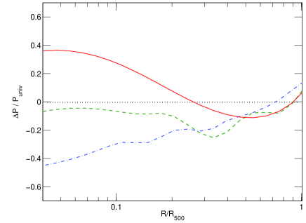
Figure 4: Comparison of simulated and semi-analytic gas pressure profiles with observed ’Universal’ pressure profile by Arnaud et al. (2009) for a cluster having $M_{500}=2\times 10^{14}h^{-1}M_{\odot}$. Plotted are the fractional differences of our fiducial model given by red solid line, the profiles obtained from simulations by Battaglia et al. (2010) (green dashed line) and Sehgal et al. (2010) (blue dot-dashed line) w.r.t the universal profile found by Arnaud et al. (2009) from observations upto $r_{500}$ and simulations beyond.

4 Discussions and Conclusion

We have constructed a top-down model for galaxy clusters, normalized to the mass-temperature relation from X-Ray observations. The gas density and temperature profiles are found by iteratively solving the gas dynamical equation having both thermal and non-thermal pressure support. The form of the non-thermal pressure used is taken from Rasia et al. (2004). In our model, $f_{\rm gas}$ becomes 0.9 ($\frac{\Omega_{b}}{\Omega_{M}}$) at the cluster boundary , whereas gas is pushed out of the cluster cores to give $f_{\rm gas}(r_{500})=0.1324+0.0284$ $\rm{log}(\frac{M_{500}}{10^{15}h^{-1}M_{\odot}})$, similar to X-Ray observations.

At $r_{2500}$, the SZE scaling relations between SZE flux $Y$ and the cluster average temperature, $T_{\rm sl}$, gas mass, $M_{\rm gas}$, and total mass, $M_{\rm tot}$, show very good agreement and are within $1-\sigma$ to the best fit line to the Bonamente et al. (2008) data. Especially, for the $Y-M_{\rm gas}$ relation the agreement is excellent. In comparison, we also show that the Komatsu-Seljak model is in less agreement to the SZE scaling relations, especially for $Y-T_{\rm sl}$ and $Y-M_{\rm gas}$. Our $r_{2500}$ scaling relations can be compared to those obtained from simulations. For example, the Nagai (2006)(see their table 3 for scaling parameters) radiative simulation prediction for the $Y-M_{\rm gas}$ relation gives a $\Delta\chi^{2}=4.7$ w.r.t. to the best fit Bonamente et al. (2008) relation. Recently Bode et al. (2009) have predicted SZ scalings from a mixture of N-body simulations plus semi-analytic gas models, normalized to X-Ray observations for low-$z$ clusters. The $\Delta\chi^{2}$ of their model is 0.06 and agrees well with our results.

Further out, at $r_{500}$, the $Y-M$ scaling relation obtained for our models agree very well with those obtained from X-Ray observations (Arnaud et al., 2009). Most assuringly, the gas pressure profile in our simple phenomenological model of clusters, comes out to be within $\sim 20\%$ beyond .1 $R_{500}$ to the observed ‘Universal’ pressure profile given by Arnaud et al. (2009).

Most importantly, the fact that X-Ray normalised models can reproduce SZE scaling relations well is reassuring for cluster studies. It shows that we are looking at a common population of clusters as a whole, and there is no deficit of SZE flux relative to expectations from X-Ray scaling properties. Thus, one can compare and cross-calibrate clusters from upcoming X-Ray and SZE surveys with increased confidence. It also gives us confidence to extrapolate our models to larger radii in order to construct the $Y-M_{200}$ scaling relation and SZ power spectrum templates.

References

- Arnaud et al. (2005) Arnaud, M., Pointecouteau, E., & Pratt, G. W. 2005, A&A, 441, 893
- Arnaud et al. (2009) Arnaud, M., Pratt, G. W., Piffaretti, R., Boehringer, H., Croston, J. H., & Pointecouteau, E. 2009, ArXiv e-prints
- Ascasibar et al. (2003) Ascasibar, Y., Yepes, G., Müller, V., & Gottlöber, S. 2003, MNRAS, 346, 731
- Balogh et al. (2001) Balogh, M. L., Pearce, F. R., Bower, R. G., & Kay, S. T. 2001, MNRAS, 326, 1228
- Battaglia et al. (2010) Battaglia, N., Bond, J. R., Pfrommer, C., Sievers, J. L., & Sijacki, D. 2010, ApJ, 725, 91
- Benson et al. (2004) Benson, B. A., Church, S. E., Ade, P. A. R., Bock, J. J., Ganga, K. M., Henson, C. N., & Thompson, K. L. 2004, ApJ, 617, 829
- Binney & Tremaine (1987) Binney, J. & Tremaine, S. 1987, Galactic dynamics, ed. Binney, J. & Tremaine, S.
- Bode et al. (2009) Bode, P., Ostriker, J. P., & Vikhlinin, A. 2009, ApJ, 700, 989
- Bonaldi et al. (2007) Bonaldi, A., Tormen, G., Dolag, K., & Moscardini, L. 2007, MNRAS, 378, 1248
- Bonamente et al. (2008) Bonamente, M., Joy, M., LaRoque, S. J., Carlstrom, J. E., Nagai, D., & Marrone, D. P. 2008, ApJ, 675, 106
- Borgani et al. (2004) Borgani, S., Murante, G., Springel, V., Diaferio, A., Dolag, K., Moscardini, L., Tormen, G., Tornatore, L., & Tozzi, P. 2004, MNRAS, 348, 1078
- Bryan & Norman (1998) Bryan, G. L. & Norman, M. L. 1998, ApJ, 495, 80
- Bulbul et al. (2010) Bulbul, G. E., Hasler, N., Bonamente, M., & Joy, M. 2010, ApJ, 720, 1038
- Carlstrom et al. (2002) Carlstrom, J. E., Holder, G. P., & Reese, E. D. 2002, ARA&A, 40, 643
- Comerford & Natarajan (2007) Comerford, J. M. & Natarajan, P. 2007, MNRAS, 379, 190
- da Silva et al. (2004) da Silva, A. C., Kay, S. T., Liddle, A. R., & Thomas, P. A. 2004, MNRAS, 348, 1401
- Ettori et al. (2006) Ettori, S., Dolag, K., Borgani, S., & Murante, G. 2006, MNRAS, 365, 1021
- Komatsu & Seljak (2001) Komatsu, E. & Seljak, U. 2001, MNRAS, 327, 1353
- Komatsu et al. (2010) Komatsu, E., Smith, K. M., Dunkley, J., Bennett, C. L., Gold, B., Hinshaw, G., Jarosik, N., Larson, D., Nolta, M. R., Page, L., Spergel, D. N., Halpern, M., Hill, R. S., Kogut, A., Limon, M., Meyer, S. S., Odegard, N., Tucker, G. S., Weiland, J. L., Wollack, E., & Wright, E. L. 2010, ArXiv e-prints
- Kravtsov et al. (2005) Kravtsov, A. V., Nagai, D., & Vikhlinin, A. A. 2005, ApJ, 625, 588
- Lau et al. (2009) Lau, E. T., Kravtsov, A. V., & Nagai, D. 2009, ApJ, 705, 1129
- Leccardi & Molendi (2008) Leccardi, A. & Molendi, S. 2008, A&A, 486, 359
- Lima & Hu (2004) Lima, M. & Hu, W. 2004, Phys. Rev. D, 70, 043504
- Mahdavi et al. (2008) Mahdavi, A., Hoekstra, H., Babul, A., & Henry, J. P. 2008, MNRAS, 384, 1567
- Majumdar & Mohr (2003) Majumdar, S. & Mohr, J. J. 2003, ApJ, 585, 603
- Majumdar & Mohr (2004) —. 2004, ApJ, 613, 41
- Marrone et al. (2009) Marrone, D. P., Smith, G. P., Richard, J., Joy, M., Bonamente, M., Hasler, N., Hamilton-Morris, V., Kneib, J., Culverhouse, T., Carlstrom, J. E., Greer, C., Hawkins, D., Hennessy, R., Lamb, J. W., Leitch, E. M., Loh, M., Miller, A., Mroczkowski, T., Muchovej, S., Pryke, C., Sharp, M. K., & Woody, D. 2009, ApJ, 701, L114
- Mazzotta et al. (2004) Mazzotta, P., Rasia, E., Moscardini, L., & Tormen, G. 2004, MNRAS, 354, 10
- Nagai (2006) Nagai, D. 2006, ApJ, 650, 538
- Nagai et al. (2007) Nagai, D., Vikhlinin, A., & Kravtsov, A. V. 2007, ApJ, 655, 98
- Nath & Majumdar (2010) Nath, B. B. & Majumdar, S. 2010, in preparation
- Navarro et al. (1997) Navarro, J. F., Frenk, C. S., & White, S. D. M. 1997, ApJ, 490, 493
- Ostriker et al. (2005) Ostriker, J. P., Bode, P., & Babul, A. 2005, ApJ, 634, 964
- Peebles (1980) Peebles, P. J. E. 1980, The large-scale structure of the universe, ed. P. J. E. Peebles
- Pratt et al. (2007) Pratt, G. W., Böhringer, H., Croston, J. H., Arnaud, M., Borgani, S., Finoguenov, A., & Temple, R. F. 2007, A&A, 461, 71
- Puchwein et al. (2008) Puchwein, E., Sijacki, D., & Springel, V. 2008, ApJ, 687, L53
- Rasheed et al. (2010) Rasheed, B., Bahcall, N., & Bode, P. 2010, ArXiv e-prints, 1007.1980
- Rasia et al. (2004) Rasia, E., Tormen, G., & Moscardini, L. 2004, MNRAS, 351, 237
- Sanderson & Ponman (2010) Sanderson, A. J. R. & Ponman, T. J. 2010, MNRAS, 402, 65
- Sanderson et al. (2006) Sanderson, A. J. R., Ponman, T. J., & O’Sullivan, E. 2006, MNRAS, 372, 1496
- Sehgal et al. (2010) Sehgal, N., Bode, P., Das, S., Hernandez-Monteagudo, C., Huffenberger, K., Lin, Y., Ostriker, J. P., & Trac, H. 2010, ApJ, 709, 920
- Sun et al. (2009) Sun, M., Voit, G. M., Donahue, M., Jones, C., Forman, W., & Vikhlinin, A. 2009, ApJ, 693, 1142
- Sunyaev & Zeldovich (1980) Sunyaev, R. A. & Zeldovich, I. B. 1980, ARA&A, 18, 537
- Verde et al. (2002) Verde, L., Haiman, Z., & Spergel, D. N. 2002, ApJ, 581, 5
- Vikhlinin et al. (2006) Vikhlinin, A., Kravtsov, A., Forman, W., Jones, C., Markevitch, M., Murray, S. S., & Van Speybroeck, L. 2006, ApJ, 640, 691
- Vikhlinin et al. (2009) Vikhlinin, A., Burenin, R. A., Ebeling, H., Forman, W. R., Hornstrup, A., Jones, C., Kravtsov, A. V., Murray, S. S., Nagai, D., Quintana, H., & Voevodkin, A. 2009, ApJ, 692, 1033
- Zhang et al. (2008) Zhang, Y., Finoguenov, A., Böhringer, H., Kneib, J., Smith, G. P., Kneissl, R., Okabe, N., & Dahle, H. 2008, A&A, 482, 451