A majorization–minimization approach to variable selection using spike and slab priors

Abstract

We develop a method to carry out MAP estimation for a class of Bayesian regression models in which coefficients are assigned with Gaussian-based spike and slab priors. The objective function in the corresponding optimization problem has a Lagrangian form in that regression coefficients are regularized by a mixture of squared $l_{2}$ and $l_{0}$ norms. A tight approximation to the $l_{0}$ norm using majorization–minimization techniques is derived, and a coordinate descent algorithm in conjunction with a soft-thresholding scheme is used in searching for the optimizer of the approximate objective. Simulation studies show that the proposed method can lead to more accurate variable selection than other benchmark methods. Theoretical results show that under regular conditions, sign consistency can be established, even when the Irrepresentable Condition is violated. Results on posterior model consistency and estimation consistency, and an extension to parameter estimation in the generalized linear models are provided.

T1Supported in part by Grants NSC 97-3112-B-001-020 and NSC 98-3112-B-001-027 in the National Research Program for Genomic Medicine.

1 Introduction

Consider the following regression model:

$$Y_{i}=x_{i1}\beta_{1}+x_{i2}\beta_{2}+\cdots+x_{ip}\beta_{p}+\varepsilon_{i},$$ (1)

where $Y_{i}$ is the response variable for the $i$th subject, $x_{ij}$ is the $j$th covariate for the $i$th subject, $\beta_{j}$ is the corresponding regression coefficient and $\varepsilon_{i}$ is the error term following some specified distribution. Variable selection in regression problems has long been considered as one of the most important issues in modern statistics. It involves choosing an appropriate subset $\widehat{S}$ of indices $\{1,2,\ldots,p\}$ so that for $j\in\widehat{S}$, the covariates $x_{ij}$’s and estimated coefficients $\widehat{\beta}_{j}$’s are scientifically meaningful in interpretation, and estimates $\widehat{y}_{i^{\prime}}=\sum_{j\in\widehat{S}}x_{i^{\prime}j}\widehat{\beta}_{j}$ have relative good properties in prediction.

In this paper, we develop a method to carrying out maximum a posteriori (MAP) estimation for a class of Bayesian models in tackling variable selection problems. The use of MAP estimation in variable selection problems had previously been studied by Genkin et al. genkinetal07 on logistic regression models with Laplace priors. The difference between our model and Genkin et al.’s is that our model assigns a Gaussian-based spike and slab prior weighted by Bernoulli variables on each regression coefficient. Traditionally, parameter estimation for this model and other Bayesian variable selection settings relies on Markov chain Monte Carlo for posterior simulation georgeandmcculloch93 , georgeandmcculloch97 , parkandcasella08 , hans09 , liandlin10 , griffinandbrown10 and empirical Bayes methods georgeandfoster00 , clydeandgeorge00 , johnstoneandsilverman05 . A major advantage of MCMC-based inference procedures is that they provide a practical way to assessing posterior probabilities, and inference tasks such as point estimation can be carried out straightforwardly based on posterior probability calculation. However, convergence of MCMC-based sampling algorithms is not often guaranteed and they may become time-consuming as the number of covariates $p$ becomes quite large. A different inference procedure on models with spike and slab priors is recently provided by Ishwaran and Rao ishwaranandrao05a , ishwaranandrao05b , in that regression coefficients are estimated via OLS-based shrinkage methods.

Our estimation method is different from the above approaches in several aspects. In our MAP estimation, an augmented version of the posterior joint density is derived. From frequentists’ point of view, the MAP estimation is equivalent to the regularization estimation with a mixture penalty of squared $l_{2}$ and $l_{0}$ norms on regression coefficients. In practice, we apply a majorization–minimization technique to modify the penalty function so that convexity of the objective function can be achieved. We then construct a coordinate descent algorithm based on a specified iteration scheme to obtain the MAP estimate. The algorithm involves iteratively applying shrinkage-thresholding steps to obtain estimates that have sparse features, that is, some of them have exact zero values. In this sense, parameter estimation and variable selection can be achieved simultaneously. In addition, the algorithm can be implemented practically in a situation in which the number of covariates $p$ is much larger than the number of samples $n$. It is different from the OLS-based methods in that $p\leq n$ is required to avoid singularity in matrix operation. The algorithm can also be fast when $p$ is large but the number of covariates with nonzero coefficients is small. Simulation studies show that the MAP estimate can lead to better performances in variable selection than those based on other benchmark methods in various circumstances.

Recent frequentists’ approaches to variable selection focus on applying the idea of regularization estimation in the situation in which the number of variables is much larger than the number of samples fanandli01 , zouandli08 , zouandhastie05 , zouandzhang09 , friedmanetal09 , zou06 , yuanandlin06 , meieretal08 , candesandtao07 , meinshausen07 , zhang10 . All these approaches can either been seen as alternatives or as extensions of the lasso estimation tibshirani96 . For theoretical properties of the lasso estimation, Knight and Fu knightandfu00 pointed out that with regular conditions on the order magnitude of the tuning parameter, the lasso is consistent in parameter estimation. However, as shown by Meinshausen and Bühlmann meinshausenandbuhlmann06 and Zou zou06 , for the lasso estimation, consistency in parameter estimation does not imply consistency in variable selection. Further conditions on the design matrix and tuning parameter should be imposed to ensure consistency in variable selection for the lasso estimation. In this aspect, Zhao and Yu zhaoandyu06 established the Irrepresentable Condition and showed that the lasso can be asymptotically consistent in both variable selection and parameter estimation if the Irrepresentable Condition holds and some regular conditions on the tuning parameter are satisfied. The same condition was also established by Zou zou06 and Yuan and Lin yuanandlin07 . Later we will show that the MAP estimator proposed in this paper is asymptotically consistent in variable selection even when frequentists’ Irrepresentable Condition is violated.

The paper is organized as follows. Section 3 focuses methodological aspects of the proposed method. Section 4 provides two simulation studies on performances of the proposed method. Section 5 develops relevant asymptotic analysis for the method. Section 6 extends the method to parameter estimation in the generalized linear models. Real data examples are provided in Section 7. Some concluding remarks are given in Section 8.

2 Notation

Let $X$ be an $n\times p$ design matrix. Let $x_{i}$ denote the $i$th row of $X$ and $x_{ij}$ denote the $ij$th entry of $X$. The transpose of $X$ is denoted by $X^{T}$. Let $y=(y_{1},y_{2},\ldots,y_{n})$ denote the realization of random vector $Y=(Y_{1},Y_{2},\ldots,Y_{n})$ and $\beta=(\beta_{1},\beta_{2},\ldots,\beta_{p})$ denote the regression coefficient vector. Let $I_{p\times p}$ denote the $p\times p$ identity matrix. For a $p$-dimensional vector $a=(a_{1},a_{2},\ldots,a_{p})$, define the $l_{1}$ norm by $\|a\|_{1}=\sum_{j=1}^{p}|a_{j}|$, the $l_{2}$ norm by $\|a\|_{2}=(\sum_{j=1}^{p}|a_{j}|^{2})^{1/2}$, the $l_{\infty}$ norm by $\|a\|_{\infty}=\max_{j}|a_{j}|$ and the $l_{0}$ norm by $\|a_{j}\|_{0}=\sum_{j=1}^{p}\mathbb{I}(a_{j}\neq 0)$, where $\mathbb{I}(a_{j}\neq 0)$ is an index variable such that $\mathbb{I}(a_{j}\neq 0)=1$ if $a_{j}\neq 0$ and $\mathbb{I}(a_{j}\neq 0)=0$ otherwise. The probability density of a random variable $Z$ conditional on $\theta$ is denoted by $f(z|\theta)$. We define $S=\{j\dvtx\beta_{j}\neq 0,j=1,2,\ldots,p\}$, that is, the index set of nonzero valued coefficients in $\beta=(\beta_{1},\beta_{2},\ldots,\beta_{p})$. We further define $X_{S}$ as the design matrix of $X$ whose columns are indexed by $S$. Finally, we define the sign function for variable $z$ as $\operatorname{sign}(z)=1$ if $z>0$; $\operatorname{sign}(z)=-1$ if $z<0$; $\operatorname{sign}(z)=0$ if $z=0$.

3 The method

We start by assigning prior distributions on parameters in the regression model (1). Note that in a regression model a covariate can only be selected if its coefficient is estimated with a nonzero value. Based on this observation, we assign an index variable $\gamma_{j}$ to each covariate and define that $\gamma_{j}=1$ if $\beta_{j}\neq 0$ and $\gamma_{j}=0$ if $\beta_{j}=0$. Here, we may write $\gamma_{j}=\mathbb{I}(\beta_{j}\neq 0)$. With the definition of $\gamma_{j}$, the regression model (1) has an equivalent representation given by

$$Y_{i}=\sum_{j=1}^{p}x_{ij}\gamma_{j}\beta_{j}+\varepsilon_{i}.$$

From a variable selection point of view, the index vector $\gamma=(\gamma_{1},\gamma_{2},\ldots,\gamma_{p})$ is an indicator for candidate models. Different candidate models will have different values in $\gamma$.

3.1 The Bayesian formulation

Under a Bayesian framework, we assume

$$Y_{i}|x_{i},\beta,\gamma,\sigma^{2} \sim \operatorname{Normal}\Biggl{(}\sum_{j=1}^{p}x_{ij}\gamma_{j}\beta_{j},\sigma^{2}\Biggr{)}\qquad\mbox{for }i=1,2,\ldots,n,$$

$$\beta_{j}|\sigma^{2},\gamma_{j},\lambda \sim \gamma_{j}\operatorname{Normal}(0,\sigma^{2}\lambda^{-1})+(1-\gamma_{j})\mathbb{I}(\beta_{j}=0)$$ (2)

$$\hskip 168.0pt\mbox{for }j=1,2,\ldots,p,$$

$$\sigma^{2}|\tau_{1},\tau_{2} \sim \mathrm{Inverse\mbox{-}Gamma}(\tau_{1},\tau_{2}),$$

$$\gamma_{j}|\kappa \sim \operatorname{Bernoulli}(\kappa)\qquad\mbox{for }j=1,2,\ldots,p.$$

The prior distribution of $\beta_{j}$ given in (3.1) is the spike and slab prior originally proposed by Mitchell and Beauchamp mitchellandbeauchamp88 . It implies that conditional on $\gamma_{j}=0$, $\beta_{j}$ is equal to 0 with probability one, and conditional on $\gamma_{j}=1$, $\beta_{j}$ follows a normal distribution with mean $0$ and variance $\sigma^{2}\lambda^{-1}$. The Bernoulli prior on $\gamma_{j}$ says that if only prior information is available, $\gamma_{j}$ will have probability $\kappa$ to be 1 and $1-\kappa$ to be 0. Note that since $\gamma_{j}\in\{0,1\}$, we can express the mixture form of the prior on $\beta_{j}$ as $\operatorname{Normal}(0,\sigma^{2}\lambda^{-1})^{\gamma_{j}}\times\mathbb{I}(\beta_{j}=0)^{1-\gamma_{j}}$. This representation will be used in deriving the joint posterior density of the parameters.

Under Bayesian model (3.1), the joint posterior density of $\beta$, $\gamma$ and $\sigma^{2}$ can be expressed as

$$f(\beta,\gamma,\sigma^{2}|X,y,\lambda,\tau_{1},\tau_{2},\kappa)$$

(3)

$$\qquad\propto f(y|X,\beta,\gamma,\sigma^{2})f(\beta|\sigma^{2},\gamma,\lambda)f(\sigma^{2}|\tau_{1},\tau_{2})f(\gamma|\kappa).$$

With (3.1), we can estimate $(\beta,\gamma,\sigma^{2})$ via various inference methods. In this paper, the maximum a posteriori (MAP) method is adopted. Formally, the MAP estimator for $(\beta,\gamma,\sigma^{2})$ is defined by

$$(\widehat{\beta},\widehat{\gamma},\widehat{\sigma}^{2})=\arg\min_{\beta,\gamma,\sigma^{2}}\{-2\log f(\beta,\gamma,\sigma^{2}|X,y,\lambda,\tau_{1},\tau_{2},\kappa)\},$$ (4)

that is, the minimizer of the minus 2 logarithm of the joint posterior density. The minus 2 logarithm of the joint posterior density can be explicitly expressed as

$$-2\log f(\beta,\gamma,\sigma^{2}|X,y,\lambda,\tau_{1},\tau_{2},\kappa) = \frac{1}{\sigma^{2}}\sum_{i=1}^{n}\Biggl{(}y_{i}-\sum_{j=1}^{p}x_{ij}\gamma_{j}\beta_{j}\Biggr{)}^{2}$$

$${}+\frac{\lambda}{\sigma^{2}}\sum_{j=1}^{p}\gamma_{j}\beta_{j}^{2}$$

$${}+\frac{2\tau_{2}}{\sigma^{2}}+(n+2\tau_{1}+2)\log\sigma^{2}$$

$${}+\sum_{j=1}^{p}\gamma_{j}\log\biggl{\{}\frac{2\pi\sigma^{2}(1-\kappa)^{2}}{\lambda\kappa^{2}}\biggr{\}}+\mathrm{const}.$$

Here, we have used an equivalent representation $\operatorname{Normal}(0,\sigma^{2}\lambda^{-1})^{\gamma_{j}}\times\mathbb{I}(\beta_{j}=0)^{1-\gamma_{j}}$ for $f(\beta_{j}|\sigma^{2},\lambda,\gamma)$ given that $\gamma_{j}\in\{0,1\}$. Note that in (3.1) the term $\sum_{j=1}^{p}\log\mathbb{I}(\beta_{j}=0)^{1-\gamma_{j}}$ vanishes since for every $j$, $\gamma_{j}=1$ implies $\mathbb{I}(\beta_{j}=0)=0$. In turn, $(1-\gamma_{j})\log\mathbb{I}(\beta_{j}=0)=0\cdot\infty=0$. On the other hand, $\gamma_{j}=0$ implies $\mathbb{I}(\beta_{j}=0)=1$, and in turn $\log\mathbb{I}(\beta_{j}=0)=\log 1=0$.

For practical purposes, we fix $\sigma^{2}$ and multiply (3.1) with $\sigma^{2}$ in the following discussion. Given that $\sigma^{2}$ is fixed, the function (3.1) has some meaningful interpretations in terms of regularization estimation on $\beta$. For example, by definition $\gamma_{j}\geq 0$, and the quantity $\sum_{j=1}^{p}\gamma_{j}$ can be seen as an $l_{1}$ norm on the vector $\gamma$. Given the above argument, we can write the fourth term on the right-hand side of (3.1) as $\rho_{\lambda,\kappa,\sigma^{2}}\|\gamma\|_{1}$, where $\rho_{\lambda,\kappa,\sigma^{2}}=\sigma^{2}\log[2\pi\sigma^{2}\lambda^{-1}(1-\kappa)^{2}\kappa^{-2}]$. Note that as $\kappa$ increases, $\rho_{\lambda,\kappa,\sigma^{2}}$ will decrease. It implies that a strong belief in the presence of a variable will decrease the penalty value for the variable. In addition, by definition $\gamma_{j}=\mathbb{I}(\beta_{j}\neq 0)$, and the term $\|\gamma\|_{1}$ can further be seen as an $l_{0}$ norm on $\beta$, as $\|\gamma\|_{1}=\sum_{j=1}^{p}|\mathbb{I}(\beta_{j}\neq 0)|=\lim_{s\rightarrow 0}\sum_{j=1}^{p}\beta_{j}^{s}$, which is the $l_{0}$ norm by definition. Here, we have used the assumption that $0^{0}=0$. We can express the fourth term in (3.1) by $\rho_{\lambda,\kappa,\sigma^{2}}\|\beta\|_{0}$.

3.2 Parameter estimation

Now given all other parameters fixed, the MAP estimator of $\sigma^{2}$ can be derived by first making a derivative of (3.1) with respect to $\sigma^{2}$, setting the derivative to zero, and then solving the equation for $\sigma^{2}$. The estimation of $\beta$ is further carried out given $\sigma^{2}$ is fixed. With fixed $\sigma^{2}$ and the interpretations of regularization estimation given above, (3.1) has an equivalent representation given by

$$L(\beta;\lambda,\rho_{\lambda,\kappa,\sigma^{2}})=\|y-X\beta\|_{2}^{2}+\lambda\|\beta\|_{2}^{2}+\rho_{\lambda,\kappa,\sigma^{2}}\|\beta\|_{0}+\mathrm{const}.$$ (6)

Note that here we have multiplied (3.1) with $\sigma^{2}$. Now with (6), we can construct an iteration scheme to obtain (4). At the $(m+1)$th iteration, the iteration scheme is given by

$$(\widehat{\sigma}^{2})^{(m+1)} = \frac{\sum_{i=1}^{n}(y_{i}-\sum_{j=1}^{p}x_{ij}\widehat{\gamma}_{j}^{(m)}\widehat{\beta}_{j}^{(m)})^{2}+\lambda\sum_{j=1}^{p}\widehat{\gamma}_{j}^{(m)}(\widehat{\beta}_{j}^{(m)})^{2}+2\tau_{2}}{n+\sum_{j=1}^{p}\widehat{\gamma}_{j}^{(m)}+2\tau_{1}+2},$$

$$\widehat{\beta}^{(m+1)} = \arg\min_{\beta}L\bigl{(}\beta;\lambda,\rho_{\lambda,\kappa,(\widehat{\sigma}^{2})^{(m+1)}}\bigr{)},$$ (7)

$$\widehat{\gamma}^{(m+1)} = \bigl{(}\mathbb{I}\bigl{(}\widehat{\beta}_{1}^{(m+1)}\neq 0\bigr{)},\mathbb{I}\bigl{(}\widehat{\beta}_{2}^{(m+1)}\neq 0\bigr{)},\ldots,\mathbb{I}\bigl{(}\widehat{\beta}_{p}^{(m+1)}\neq 0\bigr{)}\bigr{)}.$$

Note that the objective function (6) involves an $l_{0}$ norm, which by definition, is not continuous. Therefore, related optimization tasks in the second term of (3.2) require some refinements. Here, we adopt a relaxation approach to tackling the optimization problem. We begins the approach by noting that, mathematically the $l_{0}$ norm on a $p$-dimensional vector $\beta$ can be expressed as

$$\|\beta\|_{0}=\lim_{\tau_{3}\rightarrow 0}\sum_{j=1}^{p}\frac{\log(1+\tau_{3}^{-1}|\beta_{j}|)}{\log(1+\tau_{3}^{-1})},$$ (8)

which can be verified by seeing (8) as a function of $\tau_{3}$ and using l’Hôpital’s rule. A more detailed discussion on the properties of the log-sum function on the right-hand side of (8) is given in Supplementary Material sup . With representation (8), the objective function (6) can be reexpressed as

$$L(\beta;\lambda,\rho_{\lambda,\kappa,\sigma^{2}}) = \|y-X\beta\|_{2}^{2}+\lambda\|\beta\|_{2}^{2}$$

$${}+\rho_{\lambda,\kappa,\sigma^{2}}\Biggl{\{}\lim_{\tau_{3}\rightarrow 0}\sum_{j=1}^{p}\frac{\log(1+\tau_{3}^{-1}|\beta_{j}|)}{\log(1+\tau_{3}^{-1})}\Biggr{\}}+\mathrm{const}.$$

If $\tau_{3}$ is small enough, the log-sum function on the right-hand side of (3.2) will give an approximate representation of $\|\beta\|_{0}$. Graphical representations for the log-sum function with different $\tau_{3}$ and their mixtures with the squared $l_{2}$ norm can be found in the left and middle panels of Figure 1. In addition, since the log-sum function in (3.2) is continuous in $\beta$, the combinatorial nature of $\|\beta\|_{0}$ is relaxed. However, the term $\log(1+\tau_{3}^{-1}|\beta_{j}|)$ is not convex in $\beta_{j}$, and replacing $\|\beta\|_{0}$ with (8) in (6) still makes objective function (3.2) remain nonconvex. To tackle this problem, a majorization–minimization algorithm is adopted. Majorization-minimization (MM) algorithms hunterandlange05 , wuandlange08 are a set of analytic procedures aiming to tackle difficult optimization problems by modifying their objective functions so that solution spaces of the modified ones are easier to explore. For an objective function $g(\theta)$, the modification procedure relies on finding a function $h(\theta;\theta^{(l)})$ satisfying the following properties:

$$h\bigl{(}\theta;\theta^{(l)}\bigr{)} \geq g(\theta)\qquad\mbox{for all }\theta,$$

$$h\bigl{(}\theta^{(l)};\theta^{(l)}\bigr{)} = g\bigl{(}\theta^{(l)}\bigr{)}.$$

In (3.2), the objective function $g(\theta)$ is said to be majorized by $h(\theta;\theta^{(l)})$. In this sense, $h(\theta;\theta^{(l)})$ is called the majorization function. In addition, (3.2) implies that $h(\theta;\theta^{(l)})$ is tangent to $g(\theta)$ at $\theta^{(l)}$. Moreover, if $\theta^{(l+1)}$ is a minimizer of $h(\theta;\theta^{(l)})$, then (3.2) further implies that

$$g\bigl{(}\theta^{(l)}\bigr{)}=h\bigl{(}\theta^{(l)};\theta^{(l)}\bigr{)}\geq h\bigl{(}\theta^{(l+1)};\theta^{(l)}\bigr{)}\geq g\bigl{(}\theta^{(l+1)}\bigr{)},$$ (11)

which means that the iteration procedure $\theta^{(l)}$ pushes $g(\theta)$ toward its minimum.

Now we turn back to the function on the right-hand side of (3.2). Note that, since $\log(\theta)$ is a concave function of $\theta$ for $\theta>0$, therefore the inequality

$$\log(\theta^{\prime})+\frac{\theta}{\theta^{\prime}}-1\geq\log(\theta)$$ (12)

holds for all $\theta>0$ and $\theta^{\prime}>0$. Note that the left-hand side of (12) is convex in $\theta$. In addition, if we let $\theta^{\prime}=\theta$, then (12) becomes an equality, which implies that the left-hand side of (12) satisfies the properties stated in (3.2), therefore is a valid function for majorizing $\log(\theta)$.

Proposition 3.1

Define $\rho_{\tau_{3}}=1/\log(1+\tau_{3}^{-1})$ and let $L^{\prime}(\beta;\lambda,\rho_{\lambda,\kappa,\sigma^{2}})$ be the same as (6) but without the constant term. Then $L^{\prime}(\beta;\lambda,\rho_{\lambda,\kappa,\sigma^{2}})$ can be majorized by the following function:

$$L^{\prime\prime}(\beta;\lambda,\rho_{\lambda,\kappa,\sigma^{2}},\beta^{\prime})=\|y-X\beta\|_{2}^{2}+\lambda\|\beta\|_{2}^{2}+\rho_{\lambda,\kappa,\sigma^{2}}h_{2}(\beta;\beta^{\prime}),$$ (13)

where

$$h_{2}(\beta;\beta^{\prime})=\lim_{\tau_{3}\rightarrow 0}\rho_{\tau_{3}}\sum_{j=1}^{p}\biggl{(}\log(1+\tau_{3}^{-1}|\beta_{j}^{\prime}|)+\frac{|\beta_{j}|+\tau_{3}}{|\beta_{j}^{\prime}|+\tau_{3}}-1\biggr{)}.$$ (14)

Let $h_{1}(\beta)=\|y-X\beta\|_{2}^{2}+\lambda\|\beta\|_{2}^{2}$. Assume $\beta^{(l+1)}$ minimizes $L^{\prime\prime}(\beta;\break\lambda,\rho_{\lambda,\kappa,\sigma^{2}},\beta^{\prime})$ given $\beta^{\prime}=\beta^{(l)}$. Then with (8) and the inequality (12), the quantity $L^{\prime}(\beta^{(l+1)};\lambda,\rho_{\lambda,\kappa,\sigma^{2}})$ can be bounded in a way such that

$$L^{\prime}\bigl{(}\beta^{(l+1)};\lambda,\rho_{\lambda,\kappa,\sigma^{2}}\bigr{)} = h_{1}\bigl{(}\beta^{(l+1)}\bigr{)}+\rho_{\lambda,\kappa,\sigma^{2}}\lim_{\tau_{3}\rightarrow 0}\rho_{\tau_{3}}\sum_{j=1}^{p}\log\bigl{(}1+\tau_{3}^{-1}\bigl{|}\beta_{j}^{(l+1)}\bigr{|}\bigr{)}$$

$$\leq h_{1}\bigl{(}\beta^{(l+1)}\bigr{)}+\rho_{\lambda,\kappa,\sigma^{2}}h_{2}\bigl{(}\beta^{(l+1)};\beta^{(l)}\bigr{)}$$

$$= L^{\prime\prime}\bigl{(}\beta^{(l+1)};\lambda,\rho_{\lambda,\kappa,\sigma^{2}},\beta^{(l)}\bigr{)}$$

which verifies the first condition stated in (3.2). For $\beta=\beta^{\prime}$, $h_{2}(\beta;\beta^{\prime})$ is equal to the log-sum function in (8), which verifies the second condition stated in (3.2) and completes the proof.

A graphical representation of using MM algorithms in approximating the log-sum function in (8) can be found in the right panel of Figure 1. From the argument given above, we can construct an iteration scheme to obtain the minimizer of $L(\beta;\lambda,\rho_{\lambda,\kappa,\sigma^{2}})$, with the $l_{0}$ norm, or equivalently the log-sum function, replaced by $h_{2}(\beta;\beta^{\prime})$ defined in Proposition 3.1. For example, in (3.2), $\widehat{\beta}^{(m+1)}$ can be obtained by carrying out the following iteration scheme:

$$\widehat{\beta}^{(m+1,l+1)}$$

$$\qquad=\arg\min_{\beta}\Biggl{\{}\|y-X\beta\|_{2}^{2}+\lambda\|\beta\|_{2}^{2}+\rho_{\lambda,\kappa,(\widehat{\sigma}^{2})^{(m+1)}}\sum_{j=1}^{p}\widehat{\phi}_{j}^{(m+1,l)}|\beta_{j}|\Biggr{\}}$$

over index $l$, where $\widehat{\phi}_{j}^{(m+1,l)}=\lim_{\tau_{3}\rightarrow 0}[\log(1+\tau_{3}^{-1})(|\widehat{\beta}_{j}^{(m+1,l)}|+\tau_{3})]^{-1}$. The procedure of using iteration scheme (3.2) in obtaining the minimizer for the objective function (6), or equivalent (3.2), is called the BAVA-MIO (BAyesian VAriable selection using a Majorization–mInimization apprOach), and the resulting minimizer is called the BAVA-MIO estimator.

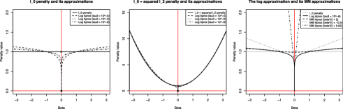
Figure 1: The penalty functions and related approximations.

Note that the last term on the right-hand side of (3.2) is a linear combination of $\widehat{\phi}_{j}^{(m+1,l)}|\beta_{j}|$, a convex function of $\beta_{j}$, therefore given $\|y-X\beta\|_{2}^{2}+\lambda\|\beta\|_{2}^{2}$ is convex in $\beta$, the whole objective function in (3.2) will be convex in $\beta$, which guarantees that the iteration scheme will converge. In addition, the minimizer (3.2) can be obtained by using the coordinate descent algorithm proposed by Friedman et al. friedmanetal07 . In practice, the coordinate descent algorithm is based on iteratively cycling a one-dimensional soft-thresholding scheme. Given that $\rho_{\lambda,\kappa,\sigma^{2}}$ is fixed, at the $(m_{1}+1)$th iteration, the soft-thresholding scheme for the $j$th coordinate is given by

$$\quad\tilde{\beta}_{j}^{(m_{1}+1)}=\Biggl{(}\sum_{i=1}^{n}x_{ij}^{2}+\lambda\Biggr{)}^{-1}\operatorname{ST}\Biggl{(}\sum_{i=1}^{n}x_{ij}\tilde{r}_{i,-j}^{(m_{1})},\rho_{\lambda,\kappa,\sigma^{2}}\frac{\tilde{\phi}_{j}^{(m_{1})}}{2}\Biggr{)},$$ (17)

where $\tilde{r}_{i,-j}^{(m_{1})}=y_{i}-\sum_{j^{\prime}\neq j}x_{ij^{\prime}}\tilde{\beta}_{j^{\prime}}^{(m_{1}^{\prime})}$, with $m_{1}^{\prime}=m_{1}+1$ for $j^{\prime}=1,2,\ldots,j-1$, and $m_{1}^{\prime}=m_{1}$ for $j^{\prime}=j+1,j+2,\ldots,p$, and $\tilde{\phi}_{j}^{(m_{1})}=\lim_{\tau_{3}\rightarrow 0}[\log(1+\tau_{3}^{-1})(|\tilde{\beta}_{j}^{(m_{1})}|+\tau_{3})]^{-1}$. Here $\operatorname{ST}(a,b)$ is a soft-thresholding operator defined by $\operatorname{ST}(a,b)=\operatorname{sign}(a)(|a|-b)_{+}$. A detailed derivation of (17) is given in Appendix A of Supplementary Material sup .

3.3 Choosing hyperparameters

Choosing appropriate hyperparameters for prior construction is an important issue in many Bayesian inference problems. For hyperparameters present in the model (3.1), we consider the triple $(\lambda,\tau_{1},\tau_{2})$ first. One principle we adopt in parameterizing the hyperparameters is that as the number of samples $n$ increases, the impact of the hyperparameters in parameter estimation will become less significant. In addition, we let $\tau_{1}=\tau_{2}+1$, so that the prior expectation of $\sigma^{2}$ is equal to 1. Given these conditions, one of the possible choices is $(\lambda,\tau_{1},\tau_{2})=(1/\sqrt{n},p\log p/\sqrt{n}+1,p\log p/\sqrt{n})$. We will discuss other possible settings in the simulation study in the later section.

Now we consider the prior inclusion probability $\kappa$. In some circumstances, data-driven empirical Bayes approaches georgeandfoster00 are proposed to obtain $\kappa$, while in other circumstances full Bayesian methods that assign priors on $\kappa$ are proposed. For example, please see liangetal07 . Unlike previously proposed approaches, in which single point estimates were obtained for $\kappa$, we adopt an approach by specifying a feasible region for the function

$$\psi(\kappa)=\tfrac{1}{2}\bigl{[}\sigma^{2}\log\bigl{(}2\pi\sigma^{2}\lambda^{-1}(1-\kappa)^{2}/\kappa^{2}\bigr{)}\bigr{]}\widehat{\phi}^{(0)},$$ (18)

and carry out parameter estimation under different values of $\psi(\kappa)$. Here we have assumed $\widehat{\phi}_{j}^{(0)}=\widehat{\phi}^{(0)}$ for $j=1,2,\ldots,p$. Note that by definition the term $\widehat{\phi}_{j}^{(0)}$ is a function of the initial value $\widehat{\beta}_{j}^{(0)}$. The function $\psi(\kappa)$ is the threshold used in the soft-thresholding scheme (17). We carry out the parameter estimation with values in the feasible region and look for which values of $\psi(\kappa)$ lead to the best performance measured by criteria such as ten fold cross validation or the Bayes factor. Under this approach, estimated parameters can be seen as functions of $\kappa$ on the feasible region. Given different values of $\kappa$, curve-like paths for estimated parameters can be obtained. The main reason we adopt this “whole-path” fitting strategy is that the optimization procedure may get stuck in some stationary points. It can occur in a situation in which we need an initial value $\widehat{\phi}_{j}^{(1)}$ to run the iteration scheme (3.2). By definition, $\widehat{\phi}_{j}^{(1)}$ is a function of $\widehat{\beta}_{j}^{(1)}$, which by definition, is a function of $\psi(\kappa)$. As pointed out by Candés et al. candesetal08 and Mazumder et al. mazumderetal09 , different $\widehat{\phi}_{j}^{(1)}$ may lead to different solutions for the minimizer. Under this situation, a global minimum may not be guaranteed. By using the strategy given above, we can run the iteration scheme (3.2) with a large number of possible values of $\widehat{\phi}_{j}^{(1)}$, therefore eliminating the possibility that the solution is stuck in some local minima.

Our approach is similar to the one using a fixed grid on the tuning parameter and then running parameter estimation with different values of the tuning parameter. This fixed grid approach to tuning parameter selection has been adopted in genkinetal07 , friedmanetal07 , meieretal08 and is advocated by wuandlange08 , friedmanetal09 for fast and accurate parameter estimation.

3.4 A toy example

Here, we provide a toy example to illustrate the BAVA-MIO estimation. We let the number of samples $n=100$ and the number of covariates $p=1\mbox{,}000$. For regression coefficients $\beta=(\beta_{1},\beta_{2},\ldots,\beta_{1\mbox{,}000})$, we let $\beta_{250}=2$, $\beta_{500}=-3.2$, $\beta_{750}=-1.25$, $\beta_{1\mbox{,}000}=5.44$, and $\beta_{j}=0$ for all $j$’s $\in\{1,2,\ldots,1\mbox{,}000\}\setminus\{250,500,750,1\mbox{,}000\}$. We generate each row of $X$ independently identically from $\operatorname{MVN}(0,I_{p\times p})$, and then calculating $Y=X\beta+\varepsilon$ with $\varepsilon\sim$ $\operatorname{MVN}(0,I_{n\times n})$. For the hyperparameters, we let $\tau_{1}=0.2p\log(p)/\sqrt{n}+1$, $\tau_{2}=0.2p\log(p)/\sqrt{n}$ and $\lambda=1/\sqrt{n}$. Further let $\tau_{3}=10^{-6}$. We use 100 equal spaced points to form a grid for $\Psi(\kappa)$. We perform two BAVA-MIO estimations: one uses the Bayes factor and the other uses ten fold cross validation for tuning parameter selection. Remember the index set $S$ is defined by $S=\{j\dvtx\gamma_{j}=1\}$. We define the Bayes factor between models $\mathcal{M}_{S^{\prime}}$ and $\mathcal{M}_{S}$ by

$$\mathrm{BF}(\mathcal{M}_{S^{\prime}},\mathcal{M}_{S};y)=\frac{f(y|\gamma^{\prime},\tau_{1},\tau_{2},\kappa,\lambda)}{f(y|\gamma,\tau_{1},\tau_{2},\kappa,\lambda)},$$ (19)

where the term $f(y|\gamma,\tau_{1},\tau_{2},\kappa,\lambda)$ refers to the marginalized likelihood with $\beta$ and $\sigma^{2}$ being integrated out with respect to their prior probability measures. For the Bayesian model stated in (3.1), the marginalized likelihood has a closed form representation given by

$$f(y|\gamma,\tau_{1},\tau_{2},\kappa,\lambda) = \frac{\pi^{-n/2}}{|\lambda^{-1}X_{S}^{T}X_{S}+I_{\gamma}|^{1/2}}\frac{(2\tau_{2})^{\tau_{1}}}{\Gamma(\tau_{1})}\Gamma\biggl{(}\frac{n+2\tau_{1}}{2}\biggr{)}$$

$${}\times\bigl{(}y^{T}(\lambda^{-1}X_{S}X_{S}^{T}+I_{n})^{-1}y+2\tau_{2}\bigr{)}^{-[(n+2\tau_{1})/2]}.$$

In subsequent sections we will use the measure (19) for variable selection. In addition, for all variable selection tasks using (19), the baseline model $\mathcal{M}_{S}$ will always refer to the null model.

The results are shown in Figure 2. The path plot in the top left panel of Figure 2 shows that nonzero coefficients entered into the model earlier under the BAVA-MIO estimation. In addition, the paths of estimated coefficients behave similar to those under the hard-thresholding estimation, that is, once a coefficient is estimated to be nonzero, the corresponding estimation path makes a sharp jump to the nonthresholded value. Moreover, due to the presence of the squared $l_{2}$ norm in the objective function, the number of selected covariates can be larger than the number of samples. Throughout the estimation procedure, the maximum number of selected covariates is 831, which is much larger than the number of samples $n=100$. Here we also provide the lasso estimation for regression fitting with the same data. The results are shown in the bottom panel of Figure 2. As compared with the lasso estimation, in which 33 covariates are selected using ten fold cross validation, the BAVA-MIO estimations using the Bayes factor and ten fold cross validation correctly select covariates with nonzero coefficients. In addition, as shown in the right panel of Figure 2, values of the nonzero coefficients are also estimated more accurately under the BAVA-MIO estimations.

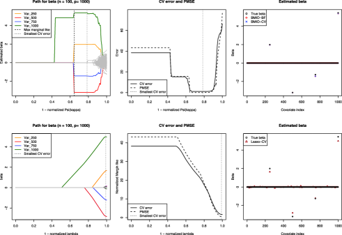
Figure 2: Estimation results for the toy example.

4 Simulation studies

In this section, we conduct two simulation studies. The first one is a general assessment on the performance of the BAVA-MIO estimation. The second one focuses the performance of the BAVA-MIO estimation under various situations in which the Irrepresentable Condition may or may not hold.

4.1 Simulation study I

In the first simulation study, we compare the BAVA-MIO estimation with other estimation approaches by fitting regression model $Y=X\beta+\varepsilon$ with data generated from different simulation schemes. Here $Y$ and $\varepsilon$ are $n$-dimensional vectors, $X$ is an $n\times p$ matrix and $\beta$ is a $p$-dimensional vector. We assume each entry in $\varepsilon$ is i.i.d. from $\operatorname{Normal}(0,\sigma_{Y}^{2})$, and each row in the design matrix $X$ is i.i.d. from $\operatorname{MVN}(0,\Sigma_{X})$. Throughout the whole simulation study, we let $p=120$. For regression coefficient vector $\beta=(\beta_{1},\beta_{2},\ldots,\beta_{p})$, we generate $\beta_{j}$ from $\operatorname{Normal}(0,1)$ for $j=1,2,\ldots,10$ and let $\beta_{j}=0$ for $j=11,12,\ldots,120$. That is, we have 10 nonzero and 110 zero coefficients in the “true” model. In addition, we use different values of $(\Sigma_{X},\sigma_{Y}^{2},n)$ in generating the design matrix $X$ and the error term $\varepsilon$. We apply three different $\Sigma_{X}$ to generate the design matrix. The first one has an independent structure with diagonal terms equal to 1 and off-diagonal terms equal to 0. The second one has a covariance structure such that $(\Sigma_{X})_{ij}=1$ for $i=j$ and $(\Sigma_{X})_{ij}=0.5$ for $i\neq j$. The third one has a covariance structure such that $(\Sigma_{X})_{ij}=0.5^{|i-j|}$. Now define the signal-to-noise ratio by SNR $=\sqrt{\mathbb{E}(\beta^{T}\Sigma_{X}\beta)/\sigma_{Y}^{2}}$. We consider $\sigma_{Y}^{2}=10,1$ and $0.2$ in generating the error term $\varepsilon$. For $\Sigma_{X}=I_{10\times 10}$, these values correspond to SNR $=1,3.16$ and $7.07$, respectively. For practical purposes, we will use the labels SNR $=1$ for experiments using $\sigma_{Y}^{2}=10$, SNR $=3.16$ for experiments using $\sigma_{Y}^{2}=1$ and SNR $=7.07$ for experiments using $\sigma_{Y}^{2}=0.2$. By using $X$, $\beta$ and $\varepsilon$, the response vector $Y$ is calculated by $Y=X\beta+\varepsilon$. For the number of samples, we consider five values $n=40,80,120,160$ and $200$. With three different structures for $\Sigma_{X}$, three different values for $\sigma_{Y}^{2}$, and five different values for $n$, we have total $3\times 3\times 5=45$ simulation experiments.

Here we describe hyperparameter settings in BAVA-MIO estimations. We let hyperparameters $(\lambda,\tau_{1},\tau_{2})=(1/\sqrt{n},p\log p/\sqrt{n}+1,p\log p/\sqrt{n})$ for the cases of SNR $=3.16$ and $7.07$. For the case of SNR $=1$, we use

$$\lambda = \biggl{(}\frac{1-\widehat{\operatorname{corr}}}{\widehat{\operatorname{corr}}}\biggr{)}^{2}\sqrt{\frac{p}{n}}\log p,$$

$$\tau_{1} = \biggl{(}\frac{\widehat{\operatorname{corr}}}{1-\widehat{\operatorname{corr}}}\biggr{)}\biggl{(}\frac{p\log p}{\sqrt{n}}\biggr{)}^{\widehat{\operatorname{corr}}/\log n}+1,$$ (20)

$$\tau_{2} = \frac{1}{\sqrt{n}}\biggl{(}\frac{p\log p}{\sqrt{n}}\biggr{)}^{1+\widehat{\operatorname{corr}}/\log n},$$

where $\widehat{\operatorname{corr}}$ is an average over the top 10 percent absolute values of the sample correlations between response $Y$ and covariates $X$. For tuning parameter selection, we use two criteria: the Bayes factor, which is defined in (19), and ten-fold cross validation. The resulting estimators are called BMIO-BF and BMIO-CV, respectively.

We also carry out three other estimation approaches for comparisons. The first one is the lasso tibshirani96 . We use R package “glmnet” to obtain the lasso estimates. The tuning parameter is selected using ten fold cross validation. The second approach is the relaxed lasso meinshausen07 . We use R package “relaxo,” which is the companion software to meinshausen07 , to obtain the relaxed lasso estimates. The tuning parameter is selected using ten fold cross validation with 100 values of scaling parameters equally spaced in $[0,1]$. The third approach is the adaptive lasso zou06 . We use R package “parcor” to obtain the adaptive lasso estimates with the default setting that uses the lasso estimate as the initial value for the weight and selects the tuning parameter $\lambda$ via ten fold cross validation.

We collect several performance measures at each simulation run. The first one is the standardized $l_{2}$ distance between a given estimate $\widehat{\beta}$ and the true regression coefficient vector $\beta$, which is defined by

$$l_{2}\mathrm{\mbox{-}dis}(\widehat{\beta})=\sqrt{\frac{\sum_{j=1}^{p}(\widehat{\beta}_{j}-\beta_{j})^{2}}{\sum_{j=1}^{p}\beta_{j}^{2}}}.$$

The second one is the predictive mean squared error of $\widehat{\beta}$ for a test data set, which is defined by

$$\operatorname{PMSE}(\widehat{\beta})=\frac{\sum_{i=1}^{n_{\mathrm{test}}}(x_{i,\mathrm{test}}^{T}\widehat{\beta}-x_{i,\mathrm{test}}^{T}\beta)^{2}}{n_{\mathrm{test}}}.$$

The test data set contains $n_{\mathrm{test}}=n\times 10$ data points generated using a simulation scheme the same as the training data set. The third one is the number of coefficients with nonzero estimated values $|\widehat{S}|$, where $\widehat{S}=\{j\dvtx\widehat{\beta}_{j}\neq 0\}$. The final one is the sign function-based false positive rates, which is defined by

$$\mathrm{S\mbox{-}FPR}=\frac{\#\{j\in\widehat{S}\dvtx\operatorname{sign}(\widehat{\beta}_{j})\neq\operatorname{sign}(\beta_{\mathrm{true},j})\}}{|\widehat{S}|},$$

where the sign function $\operatorname{sign}(\cdot)$ is defined in Section 2.

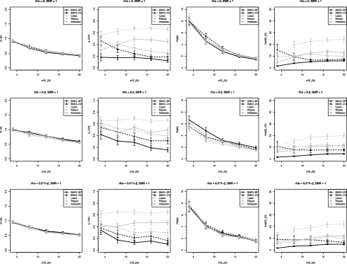
Figure 3: Simulation results given SNR $=1$. Top: Model 1 (covariance matrix with off-diagonal terms equal to $0$); Middle: Model 2 (covariance matrix with off-diagonal terms equal to $0.5$); Bottom: Model 3 (covariance matrix with off-diagonal terms following a specified covariance structure). First column: standardized $l_{2}$-distance between estimated and true values; Second column: sign function-adjusted false positive rate; Third column: prediction mean squared error; Fourth column: number of nonzero estimates.

For each of the 45 simulation experiments, we generate 100 runs to collect the four performance measures. We then plot the average of each performance measure against the ratio $n/|S|$, that is, the ratio between the number of samples and the number of true coefficients with nonzero values. These plots are shown in Figures 3, 4 and 5 for SNR $=1,3.16$ and $7.07$, respectively. From the three figures, we can see none of the estimation approaches can dominate the others in all four performance measures. In most cases, BAVA-MIO based estimations have smaller sign function-based false positive rates, as shown in the second column of each figure. It implies that more accurate variable selection may be done using the BAVA-MIO estimations. These findings become more significant as the number of samples increases. In addition, BAVA-MIO estimations have fewer numbers of nonzero estimates, as shown in the fourth column of each figure. Moreover, since the BAVA-MIO estimation using the Bayes factor has relatively fewer numbers of nonzero estimates, it is surprising that the PMSE and $l_{2}$-dis measures under the BMIO-BF estimation are comparable to those under other estimation approaches, for example, in the cases with SNR $=3.16$ and in some cases with SNR $=1$. However, we also noticed that the BMIO-BF estimation has higher values in the PMSE and $l_{2}$-dis in the cases with SNR $=7.07$, particularly in the situations in which the number of samples is small.

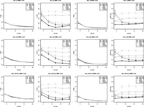
Figure 4: Simulation results given SNR $=3.16$. Top: Model 1 (covariance matrix with off-diagonal terms equal to $0$); Middle: Model 2 (covariance matrix with off-diagonal terms equal to $0.5$); Bottom: Model 3 (covariance matrix with off-diagonal terms following a specified covariance structure). First column: standardized $l_{2}$-distance between estimated and true values; Second column: sign function-adjusted false positive rate; Third column: prediction mean squared error; Fourth column: number of nonzero estimates.

Figure 5: Simulation results given SNR $=7.07$. Top: Model 1 (covariance matrix with off-diagonal terms equal to $0$); Middle: Model 2 (covariance matrix with off-diagonal terms equal to $0.5$); Bottom: Model 3 (covariance matrix with off-diagonal terms following a specified covariance structure). First column: standardized $l_{2}$-distance between estimated and true values; Second column: sign function-adjusted false positive rate; Third column: prediction mean squared error; Fourth column: number of nonzero estimates.

4.2 Simulation study II

In the second simulation study, we investigate the impact of the Irrepresentable Condition on the performance of BAVA-MIO estimation in variable selection. Before stating the Irrepresentable Condition, we give some notation definitions. We define $S_{0}=\{j\dvtx\beta_{j}\neq 0,\mbox{ for some}\break j\in\{1,2,\ldots,p\}$ and $S_{0}^{c}=\{1,2,\ldots,p\}\setminus S_{0}$. Let $\beta_{S_{0}}$ denote the coefficients with indices in $S_{0}$ and $\beta_{S_{0}^{c}}$ the coefficients with indices in $S_{0}^{c}$. Similar definitions are also applied to $X_{S_{0}}$ and $X_{S_{0}^{c}}$. An estimator $\widehat{\beta}(n)$ is said to be sign consistent in estimating $\beta$ if the probability of the event $\{\operatorname{sign}(\widehat{\beta}(n))=\operatorname{sign}(\beta)\}$ approaches to $1$ as $n\rightarrow\infty$. Given the sign consistency holds, the estimated index set $\widehat{S}_{0}=\{j\dvtx\widehat{\beta}_{j}\neq 0\}$ will be the same as the true index set $S_{0}$, therefore the sign consistency implies variable selection consistency, that is, asymptotically with probability one, nonzero-valued coefficients will have nonzero estimated values and zero-valued coefficients will be estimated with zero values.

Zhao and Yu zhaoandyu06 showed that if one wants the lasso estimation to achieve the sign consistency, then the design matrices $X$ must satisfy the following condition:

$$\|X_{S_{0}^{c}}^{T}X_{S_{0}}(X_{S_{0}}^{T}X_{S_{0}})^{-1}\operatorname{sign}(\beta_{S_{0}})\|_{\infty}<1,$$ (21)

where $\beta_{S_{0}}$ is the vector of nonzero-valued coefficients. The condition (21) is called the (Weak) Irrepresentable Condition. If the Irrepresentable Condition (21) fails to hold, then the sign consistency will never occur even when $n\rightarrow\infty$. An intuitive way to explain the Irrepresentable Condition is to see the quantity $X_{S_{0}^{c}}^{T}X_{S_{0}}(X_{S_{0}}^{T}X_{S_{0}})^{-1}$ as a least squares estimate for the regression $X_{S_{0}^{c}}$ on $X_{S_{0}}$. In this sense, the Irrepresentable Condition states that the largest amount of coefficients for the regression $X_{S_{0}^{c}}$ on $X_{S_{0}}$ should not exceed 1, that is, $X_{S_{0}^{c}}$ is “irrepresentable” in terms of $X_{S_{0}}$.

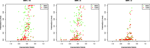
Figure 6: Scatter plots for the sign probability $\mathbb{P}(\widehat{S}=S_{0})$ against the Irrepresentable Statistic under different signal-to-noise ratios.

Here we conduct a simulation study for the investigation. We generate 100 design matrices in which each row is i.i.d. from $\operatorname{MVN}(0,\Sigma_{X})$, with $\Sigma_{X}\sim$ $\operatorname{Wishart}(I_{p\times p},p,p)$ with $p=30$. This setting is similar to the one used in Zhao and Yu’s study. Corresponding regression coefficients $\beta$ are generated in a way that the first 5 entries of $\beta$ are i.i.d. from $\operatorname{Normal}(0,1)$, and the rest of 25 entries are set to 0. Note that for some pairs $(X,\beta)$, the Irrepresentable Condition (21) will hold, but for some pairs it will not hold. Zhao and Yu defined the irrepresentable statistic by

$$\mathrm{Irr.stat}=1-\|X_{S_{0}^{c}}^{T}X_{S_{0}}(X_{S_{0}}^{T}X_{S_{0}})^{-1}\operatorname{sign}(\beta_{S_{0}})\|_{\infty}.$$ (22)

The Irrepresentable Condition is considered to be violated if Irr.stat is smaller than zero. We carry out 100 simulation runs and calculate the irrepresentable statistic for each pair $(X,\beta)$. In each run, we generate $n=100$ data points. We use $\sigma_{Y}^{2}=0.05$ to generate the error term $\varepsilon$, which is corresponding to SNR $=10$. We then fit the regression model using the lasso estimation and the BAVA-MIO estimation with these data points. For each pair $(X,\beta)$, we calculate the model selection probability $P(\widehat{S}_{0}=S_{0})$ based on counting the times of whether the estimated sign vector matched the true sign vector throughout the whole regularization paths.

We also carry out the same simulation experiment under SNR $=5$, $2$ and $1$. The scatter plots in Figure 6 show the estimated model selection probability against Irr.stat under signal-to-noise ratios SNR $=10$, $5$, and $2$. From these plots, we can see that performances of the BAVA-MIO and the lasso estimations are deteriorated when the signal-to-noise ratio is decreasing. However, we also found in some circumstances the BAVA-MIO estimation can achieve high model selection probabilities even when the Irrepresentable Condition is violated, that is, Irr.stat is smaller than zero. In Section 5, we will provide a theoretical result to explain this phenomenon. The second and fourth rows in Table 1 show the squared correlations between the estimated model selection probability and the irrepresentable statistic. The squared correlations for the BAVA-MIO estimation are relatively small in comparison with the lasso estimation.

Table 1: The sign probability $\mathbb{P}(\widehat{S}=S_{0})$ under different signal-to-noise ratios. Each value is calculated by averaging over 100 simulation runs, and the corresponding standard error is given in the bracket. The term corr. in the second line of each panel is the squared correlation between the sign probability and the irrepresentable statistic. We use Kendall’s $\tau$ for the correlation calculation

Name	$\mathbf{SNR}\bolds{=10}$	$\mathbf{SNR}\bolds{=5}$	$\mathbf{SNR}\bolds{=2}$	$\mathbf{SNR}\bolds{=1}$
BMIO	0.398 (0.030)	0.338 (0.030)	0.077 (0.018)	0.023 (0.006)
corr.	0.052 (0.030)	0.047 (0.030)	0.180 (0.030)	0.110 (0.030)
Lasso	0.314 (0.047)	0.203 (0.030)	0.072 (0.016)	0.022 (0.006)
corr.	0.418 (0.030)	0.232 (0.030)	0.194 (0.030)	0.107 (0.030)

5 Asymptotic analysis

In this section, we will derive asymptotic results for the BAVA-MIO estimator. When deriving the asymptotic results, we will consider a situation in which the number of parameters $p$ is an increasing function of the number of samples $n$. For practical purposes, we will focus on the case $p=p(n)\propto n^{\alpha}$, where $\alpha>0$. The first asymptotic result gives a theoretical explanation for the invariance of the BAVA-MIO estimator under the Irrepresentable Condition. The second result is on the posterior model consistency related to the hierarchical Bayesian formulation (3.1), and the third result shows the estimation consistency of the BAVA-MIO estimator.

5.1 Sign consistency

Before stating the result of sign consistency, we give some notation definitions first. We use the same definitions given in Section 4.2 for $S_{0}$, $S_{0}^{c}$, $\beta_{S_{0}}$, $\beta_{S_{0}^{c}}$, $X_{S_{0}}$ and $X_{S_{0}^{c}}$. Further let $\mathcal{S}$ denote the space that $S_{0}$ belongs to. For a symmetric matrix $C$, let $\Lambda_{\min}(C)$ and $\Lambda_{\max}(C)$ denote the smallest and the largest eigenvalues, respectively.

Our result on the sign consistency of the BAVA-MIO estimator is based on the following simplification: the variable $\sigma^{2}$ is fixed and the term $\rho_{\lambda,\kappa,\sigma^{2}}$ in (6) is treated as a constant. For simplicity, we let $\rho=\rho_{\lambda,\kappa,\sigma^{2}}$. Now define

$$\widehat{\beta}^{\tau_{3}}=\arg\min_{\beta}\|y-X\beta\|_{2}^{2}+\lambda\|\beta\|_{2}^{2}+\rho\sum_{j=1}^{p}\frac{\log(1+\tau_{3}^{-1}|\beta_{j}|)}{\log(1+\tau_{3}^{-1})}.$$ (23)

Note that the log-sum function on the right-hand side of (23) becomes $\|\beta\|_{0}$ if $\tau_{3}\rightarrow 0$, and $\widehat{\beta}^{\tau_{3}}$ in this sense can be seen as the BAVA-MIO estimator. Now define

$$E_{0,\tau_{3}}=\{\beta\dvtx\operatorname{sign}(\beta_{j})=\operatorname{sign}(\widehat{\beta}_{j}^{\tau_{3}})\mbox{ for }j=1,2,\ldots,p\},$$ (24)

that is, the event of sign consistency for the estimator $\widehat{\beta}^{\tau_{3}}$ in (23). For practical purposes, further define $C_{SS_{0}}=n^{-1}(X_{S_{0}}^{T}X_{S_{0}}+\lambda I)$, $C_{S^{c}S_{0}}=n^{-1}X_{S_{0}^{c}}^{T}X_{S_{0}}$, $D_{S_{0}}=n^{-1/2}X_{S_{0}}^{T}\varepsilon$ and $D_{S_{0}^{c}}=n^{-1/2}X_{S_{0}^{c}}^{T}\varepsilon$. In the following, we give some assumptions that will be used in deriving the asymptotic results.

Assumption 1.

For $C_{SS}=n^{-1}(X_{S}^{T}X_{S}+\lambda I)$ and any $S\in\mathcal{S}$, the maximum eigenvalue $\Lambda_{\max}(C_{SS})$ and the minimum eigenvalue $\Lambda_{\min}(C_{SS})$ satisfy the following condition:

$$0\leq c_{1}<\Lambda_{\min}(C_{SS})\leq\Lambda_{\max}(C_{SS})\leq c_{2}<\infty.$$

Assumption 2.

For the vector $X^{T}\varepsilon$, $\|X^{T}\varepsilon\|_{1}=O(p)$.

Assumption 3.

For parameter $\lambda$, we assume $0\leq\lambda<\infty$. For parameter $\rho$, we assume $0\leq\rho$ and $\rho n^{-1/2}\rightarrow 0$.

Assumption 1 is a special case of the Restricted Eigenvalue Assumption stated in Bickel et al. bickeletal09 . It implies that the inverse of $C_{SS_{0}}$ exists and the ratio $[\Lambda_{\max}(X_{S}^{T}X_{S})+\lambda]/[\Lambda_{\min}(X_{S}^{T}X_{S})+\lambda]\leq c_{2}/c_{1}$ is bounded from above for any $S\in\mathcal{S}$. Assumption 2 is equivalent to the statement that $n^{-1/2}\|X^{T}\varepsilon\|_{1}$ is bounded from some quantity proportional to $pn^{-1/2}$ as $n\rightarrow\infty$, which further implies $\|D_{S_{0}}\|_{1}$ and $\|D_{S_{0}^{c}}\|_{1}$ are bounded from the quantity as well.

Theorem 5.1.

Given that Assumptions 1 to 3 hold, if the number of covariates $p\propto n^{\alpha}$, $0<\alpha<1/2$, and $\tau_{3}\propto n^{-1}$, then we have

$$\mathbb{P}(E_{0,\tau_{3}})\rightarrow 1$$

as $n\rightarrow\infty$.

The proof is given in Appendix C of Supplementary Material sup . The proof will start by exploring the KKT conditions associated to the minimization problem stated in (23). Note that in Theorem 5.1 we do not assume that the Irrepresentable Condition should hold. Indeed, as stated in Corollary C1 in Appendix C, even if the Irrepresentable Condition is violated, Theorem 5.1 will still hold given that some mild condition is imposed.

5.2 Posterior model consistency

We give notation definitions first. Let $y^{n}=(y_{1},y_{2},\ldots,y_{n})$. The notation $y^{n}$ emphasizes the fact that the number of entries in the observed response vector $y$ is $n$. Further let $\mathcal{M}_{S}$ denote the model characterized by the index set $S$. Under a Bayesian framework, $\mathcal{M}_{S}$ usually refers to the sampling density, and posterior model consistency is defined as $\mathbb{P}(\mathcal{M}_{S_{0}}|y^{n})\rightarrow 1$ as $n\rightarrow\infty$, where $\mathcal{M}_{S_{0}}$ can be seen as the “true model,” or the true sampling density that a sample comes from. The posterior model consistency states that the posterior probability will put all its mass on $\mathcal{M}_{S_{0}}$ as the sample size goes to infinity. Note that in general, multiple true models are allowed under Bayesian frameworks, that is, $S_{0}$ may not be unique. However, for simplicity we only pay attention on the situation in which there is only one true model.

Note that the posterior probability $\mathbb{P}(\mathcal{M}_{S^{\prime}}|y^{n})$ with $S^{\prime}\in\mathcal{S}$ can be expressed in terms of Bayes factors by

$$\mathbb{P}(\mathcal{M}_{S^{\prime}}|y^{n}) = \frac{f(y^{n}|\mathcal{M}_{S^{\prime}})f(\mathcal{M}_{S^{\prime}})}{\sum_{S\in\mathcal{S}}f(y^{n}|\mathcal{M}_{S})f(\mathcal{M}_{S})}$$

$$= \frac{\mathrm{BF}(\mathcal{M}_{S^{\prime}},\mathcal{M}_{S_{0}};y^{n})f(\mathcal{M}_{S^{\prime}})}{\sum_{S\in\mathcal{S}}\mathrm{BF}(\mathcal{M}_{S},\mathcal{M}_{S_{0}};y^{n})f(\mathcal{M}_{S})}.$$

The formulation (5.2) implies that the event $\mathbb{P}(\mathcal{M}_{S_{0}}|y^{n})\rightarrow 1$ is equivalent to the events $\mathrm{BF}(\mathcal{M}_{S},\mathcal{M}_{S_{0}})\rightarrow 0$ for all $S\in\mathcal{S}$ and $S\neq S_{0}$, given that the probability $f(\mathcal{M}_{S_{0}})$ is bounded from zero. It turns out that to examine whether the posterior probability is consistent at the true model $\mathcal{M}_{S_{0}}$ is the same as to examine whether Bayes factors between other models and the true model will approach to zero or not.

Here, we make some assumptions on the Bayesian formulation (3.1) before stating the main result of posterior model consistency.

Assumption 4.

The prior probability on the true model $\mathcal{M}_{S_{0}}$ is bounded away from zero, that is, $f(\mathcal{M}_{S_{0}})>0$.

Assumption 5.

We assume $\lambda^{-1}\tau_{2}<\infty$.

Assumption 6.

The condition

$$\frac{(y^{n})^{T}y^{n}}{\Lambda_{\min}(X_{S_{0}}X_{S_{0}}^{T})}<(y^{n})^{T}(X_{S}X_{S}^{T}+\lambda I)^{-1}y^{n}$$

holds for all $n\in\mathbb{N}^{+}$, $S\in\mathcal{S}\setminus S_{0}$ and $0\leq\lambda<\infty$.

Assumption 4 states that the true model should always have positive mass under the prior. It is a reasonable assumption since otherwise by Bayes’ theorem the posterior probability of $\mathcal{M}_{S_{0}}$ will be zero. In addition, Assumption 6 is a technical condition which ensures that the ratio $(y^{n})^{T}(X_{S_{0}}X_{S_{0}}^{T}+\lambda I)^{-1}y^{n}/[(y^{n})^{T}(X_{S}X_{S}^{T}+\lambda I)^{-1}y^{n}]$ is smaller than 1. The assumption will be useful in proving the convergence of the Bayes factor $\operatorname{BF}(\mathcal{M}_{S},\mathcal{M}_{S_{0}};y^{n})$.

Theorem 5.2.

Given Assumptions 4 to 6 hold and the number of covariates $p\propto n^{\alpha}$, the inequality

$$\mathbb{P}(\mathcal{M}_{S_{0}}|y^{n})\geq 1-c_{3}\exp\biggl{\{}-\frac{n^{\alpha}}{2}(n^{1-\alpha}\xi-c_{11}\log 4)\biggr{\}}$$

will hold for some constants $0\leq c_{3}<\infty$, $\xi>0$, $0<c_{11}<\infty$ and $n^{*}>0$ for all $n>n^{*}$. Therefore, for $0<\alpha<1$, $\mathbb{P}(\mathcal{M}_{S_{0}}|y^{n})\rightarrow 1$ as $n\rightarrow\infty$.

The proof of Theorem 5.2 is given in Appendix D of Supplementary Material sup .

5.3 Estimation consistency

Using (23), the BAVA-MIO estimator can be defined as $\widehat{\beta}_{\mathrm{BMIO}}=\lim_{\tau_{3}\rightarrow 0}\widehat{\beta}^{\tau_{3}}$. Now we deal with the estimation consistency of $\widehat{\beta}_{\mathrm{BMIO}}$ under a frequentist’s framework. We will derive an asymptotic bound for the $l_{2}$ distance between $\widehat{\beta}_{\mathrm{BMIO}}$ and $\beta_{0}$ and show that the $l_{2}$ distance converges to 0 as $n\rightarrow\infty$. Let $\beta_{0}$ denote the coefficient vector corresponding to the true model $\mathcal{M}_{S_{0}}$. Define the expected $l_{2}$ distance between estimator $\widehat{\beta}$ and the true coefficient $\beta_{0}$ by

$$\mathbb{E}_{Y}[\|\widehat{\beta}-\beta_{0}\|_{2}^{2}]=\int\|\widehat{\beta}-\beta_{0}\|_{2}^{2}f(y|\beta_{0})\,dy,$$

where $f(y|\beta_{0})$ is the sampling density parametrized by the true parameter $\beta_{0}$. Before deriving the asymptotic result, we make some finite moment assumptions on the true parameters $(\beta_{0},\sigma^{2})$.

Assumption 7.

There exist finite constants $c_{4}>0$ and $c_{5}>0$ such that $\beta_{0,j}^{2}<c_{4}$ for $j=1,2,\ldots,p$, and $\sigma^{2}<c_{5}$.

Assumption 7 ensures that parameter $\beta_{0}$ and parameter $\sigma^{2}$ are bounded away from above as the sample size $n$ goes large.

Theorem 5.3.

Given Assumptions 1, 3 and 7 hold and the number of covariates $p\propto n^{\alpha}$ with $\alpha>0$, the inequality

$$\mathbb{P}(\|\widehat{\beta}_{\mathrm{BMIO}}-\beta_{0}\|_{2}^{2}>\xi_{n})\leq c_{13}\exp\{-\log(n^{1-\alpha}\xi_{n})\}$$ (26)

will hold for some positive finite constant $c_{13}$ and $\xi_{n}$. Assume $\xi_{n}\geq 0$ is decreasing with $n$, that is, $\xi_{n}\rightarrow 0$ as $n\rightarrow\infty$. Let $\xi_{n}\propto n^{-\alpha^{*}}$ for some $\alpha^{*}>0$. Then with the condition $0<\alpha^{*}<\alpha<1/2$, $\mathbb{P}(\|\widehat{\beta}_{\mathrm{BMIO}}-\beta_{0}\|_{2}^{2}>\xi_{n})\rightarrow 0$ as $n\rightarrow\infty$.

The proof of Theorem 5.3 is given in Appendix E of Supplementary Material sup .

6 An extension to generalized linear models

Here we extend the proposed method, the BAVA-MIO, to parameter estimation in the generalized linear models. Consider the density of the exponential family

$$f(y|\theta,\varphi)=\exp\biggl{\{}\frac{y\theta-b(\theta)}{\varphi}+d(y,\varphi)\biggr{\}},$$ (27)

where $\theta$ is a parameter characterizing mean of the distribution and $\varphi$ is a parameter characterizing dispersion of the distribution. Under the exponential family (27), variable $Y$ has properties such that $\mathbb{E}(Y|\theta,\varphi)=b^{\prime}(\theta)$, $\operatorname{Var}(Y|\theta,\varphi)=b^{\prime\prime}(\theta)\varphi$. Now let $\nu=b^{\prime}(\theta)$. For a generalized linear model, there exists a link function $\eta$ such that $\eta(\nu)=x^{T}\beta$. The link function gives a flexible connection between the mean $\nu$ and the predictor $x^{T}\beta$, and a valid regression can be formulated under this parametrization. In addition, $\nu$ is parametrized by $\theta$, therefore by inverse mapping, we can express $\theta$ as a function of $x^{T}\beta$. We write $\theta=\theta(x^{T}\beta)$.

For a practical inference concern, we will not assign a prior on $\varphi$ in the following Bayesian hierarchical formulation. We only assign priors on regression coefficients $\beta$ and covariate indices $\gamma$. The inference concern arises from the fact that the estimation of $\varphi$ is dependent on the function $d(y,\varphi)$, and in general, $d(y,\varphi)$ is case dependent. We will launch an investigation on how to assign a prior on $\varphi$ in the future, but at present we only focus on inference based on priors on $\beta$ and $\gamma$. Now consider the logarithm of the joint density function

$$-\log f(\beta,\gamma|X,y,\varphi,\lambda,\kappa) = -\sum_{i=1}^{n}\biggl{\{}\frac{y_{i}\theta_{i}(x_{i}^{T}\beta)-b[\theta_{i}(x_{i}^{T}\beta)]}{\varphi}+d(y_{i},\varphi)\biggr{\}}$$

$${}+\frac{\lambda}{2\varphi}\sum_{j=1}^{p}\gamma_{j}\beta_{j}^{2}$$

$${}+\frac{1}{2}\sum_{j=1}^{p}\gamma_{j}\log\biggl{\{}\frac{2\pi\varphi(1-\kappa)^{2}}{\lambda\kappa^{2}}\biggr{\}}+\mathrm{const}.$$

The first term in (6) is the logarithm of joint sampling density over $i=1,2,\ldots,n$, and the second and third terms are logarithms of the priors on $\beta$ and covariate indices $\gamma$, respectively. To modify (6) for BAVA-MIO estimation, we first multiply (6) with $\varphi$. We then apply a majorization–minimization technique to obtain an approximation to the $l_{0}$ norm penalty. The BAVA-MIO estimator of $\beta$ is defined as the minimizer of the approximate objective, which can be obtained by the following iteration scheme:

$$\widehat{\beta}^{(m+1)} = \arg\min\Biggl{\{}-\sum_{i=1}^{n}\{y_{i}\theta_{i}(x_{i}^{T}\beta)-b[\theta_{i}(x_{i}^{T}\beta)]\}$$

$$\hskip 71.0pt{}+\frac{\lambda}{2}\|\beta\|_{2}^{2}+\rho\|\widehat{\phi}^{(m)}\beta\|_{1}\Biggr{\}},$$

where $\rho=\varphi[\log 2\pi\varphi(1-\kappa)^{2}(\lambda\kappa^{2})^{-1}]/2$ and $\widehat{\phi}^{(m)}=\lim_{\tau_{3}\rightarrow 0}[\log(1+\tau_{3}^{-1})\times(|\widehat{\beta}^{(m)}|+\tau_{3})]^{-1}$. Further, by differentiating (6) with respect to $\beta$, and setting the derivatives to zero, we obtain the subgradient equations of $\beta$, which are given by

$$-X^{T}Wr+\lambda\beta+g_{\beta}\rho\widehat{\phi}^{(m)}=0,$$ (30)

where $r=(y-\nu)\eta^{\prime}(\nu)$, $W=\operatorname{diag}\{[\eta^{\prime}(\nu_{1})^{2}]b^{\prime\prime}(\theta_{1}),\ldots,[\eta^{\prime}(\nu_{n})^{2}]b^{\prime\prime}(\theta_{n})\}^{-1}$, $\nu=(\nu_{1},\nu_{2},\ldots,\nu_{n})$ with $\nu_{i}=b^{\prime}(\theta_{i})$ and $g_{\beta}=(g_{\beta_{1}},g_{\beta_{2}},\ldots,g_{\beta_{p}})$ is the subgradient vector of $\|\beta\|_{1}$ such that $g_{\beta_{j}}=1$ if $\beta_{j}>0$, $g_{\beta_{j}}=-1$ if $\beta_{j}<0$ and $g_{\beta_{j}}\in[-1,1]$ if $\beta_{j}=0$. The term $X^{T}Wr$ in (30) is a standard result in parameter estimation of the generalized linear models, and its derivation can be found in mccullaghandnelder89 . The term $X^{T}Wr$ allows us to formulate an iteration scheme to approximate the solution of the subgradient equations (30). Here we will use the iteration scheme

$$\qquad(\widehat{\beta}^{*})^{(m+1)}=\arg\min_{\beta}\biggl{\{}\frac{1}{2}\bigl{\|}U^{(m)}\bigl{(}z^{(m)}-X\beta\bigr{)}\bigr{\|}_{2}^{2}+\frac{\lambda}{2}\|\beta\|_{2}^{2}+\rho\bigl{\|}\widehat{\phi}^{(m)}\beta\bigr{\|}_{1}\biggr{\}},$$ (31)

where

$$z^{(m)} = r^{(m)}+\eta^{(m)},$$

$$U^{(m)} = (W^{1/2})^{(m)},$$

to approximates the solution of the subgradient equations (30). The $j$th element of the iteration scheme (31) can be obtained by further carrying out the following soft-thresholding scheme coordinatewise:

$$\quad(\tilde{\beta}_{j}^{*})^{(m+1,l+1)}=\Biggl{(}\sum_{i=1}^{n}w_{ii}^{(m)}x_{ij}^{2}+\lambda\Biggr{)}^{-1}\operatorname{ST}\Biggl{(}\sum_{i=1}^{n}x_{ij}w_{ii}^{(m)}\tilde{v}_{i,-j}^{(m,l)},\rho\tilde{\phi}_{j}^{(m)}\Biggr{)},$$ (32)

where $w_{ii}^{(m)}$ is the $i$th diagonal term of $W^{(m)}$, $\tilde{v}_{i,-j}^{(m,l)}=z_{i}^{(m)}-\sum_{j^{\prime}\neq j}x_{ij}\tilde{\beta}_{j^{\prime}}^{*}$ with $\tilde{\beta}_{j^{\prime}}^{*}=(\tilde{\beta}_{j^{\prime}}^{*})^{(m+1,l+1)}$ for $j^{\prime}=1,2,\ldots,j-1$ and $\tilde{\beta}_{j^{\prime}}^{*}=(\tilde{\beta}_{j^{\prime}}^{*})^{(m,l)}$ for $j^{\prime}=j+1,j+2,\ldots,p$, and $\operatorname{ST}(a,b)$ is the soft-thresholding operator defined by $\operatorname{ST}(a,b)=\operatorname{sign}(a)(|a|-b)_{+}$.

We now conduct a simulation study to assess the performance of the BAVA-MIO estimation. We take logistic regression as the example. For the true model, we assume $Y_{i}\sim$ $\operatorname{Bernoulli}(\zeta_{i})$, where $\zeta_{i}$ is parametrized in terms of predictor $x_{i}^{T}\beta$ via the link function $\log[(\zeta_{i})/(1-\zeta_{i})]$. We further let the number of covariates $p=120$. For the regression coefficients $\beta$, we generate the $j$th entry $\beta_{j}$ from $\operatorname{Normal}(0,1)$ for $j=1,2,\ldots,10$, and let the rest of 110 $\beta_{j}^{\prime}s$ equal to zero. We simulate covariate vector $x_{i}$ i.i.d. from $\operatorname{MVN}(0,\Sigma_{X})$. We consider three $\Sigma_{X}$’s, the same as those described in Section 4.1, to generate the covariate vectors. With $\beta$ and $x_{i}$, we simulate $Y_{i}$ from $\operatorname{Bernoulli}(\zeta_{i})$ for the cases of $n=100$ and $n=200$. With three different values for $\Sigma_{X}$ and two different values for $n$, we have six scenarios in the simulation study. For each scenario, we generate 100 simulation runs. In each simulation run, we apply the BAVA-MIO estimation to fit a logistic regression model. We let hyperparameter $\lambda=n^{-1/2}$ for all estimations. Note that for a Bernoulli variable, a closed form representation for the Bayes factor does not exist, therefore we only use ten fold cross validation for tuning parameter selection. For comparison purposes, we also carry out the lasso estimation using R package “glmnet” and use ten fold cross validation for tuning parameter selection. We collect four performance measures, the same as those described in Section 4.1, at each simulation run. Average values of the four performance measures over the 100 simulation runs are given in Table 2. From these tables we can see that the BAVA-MIO estimation in general has slightly larger values in PMSE than the lasso estimation has, but it gives far fewer number of selected covariates, more accurate results in covariate selection, and in some circumstances, better parameter estimation than the lasso estimation.

Table 2: Results of BAVA-MIO GLM estimation. Each value is calculated by averaging over 100 simulation runs, and the corresponding standard error is given in the bracket. BMIO-CV: the BAVA-MIO estimation using ten-fold cross validation; lasso: the lasso estimation. The top panel: covariance matrix with off-diagonal terms equal to $0$; The middle panel: covariance matrix with off-diagonal terms equal to $0.5$; The bottom panel: covariance matrix with off-diagonal terms following a specified covariance structure

	$\bolds{n}$	PMSE	$\bolds{l}_{\bolds{2}}$-dis	S-FPR	$\bolds{|\widehat{S}|}$
BMIO-CV	100	0.186 (0.004)	0.039 (0.002)	0.305 (0.031)	11.39 (1.788)
GLM-lasso	100	0.173 (0.003)	0.044 (0.004)	0.680 (0.012)	21.34 (1.050)
BMIO-CV	200	0.145 (0.003)	0.018 (0.001)	0.176 (0.021)	07.54 (0.549)
GLM-lasso	200	0.144 (0.002)	0.026 (0.001)	0.694 (0.011)	27.65 (1.141)
BMIO-CV	100	0.180 (0.004)	0.055 (0.003)	0.455 (0.031)	13.86 (1.841)
GLM-lasso	100	0.169 (0.003)	0.052 (0.003)	0.654 (0.018)	17.54 (0.966)
BMIO-CV	200	0.157 (0.003)	0.027 (0.002)	0.327 (0.025)	08.58 (0.564)
GLM-lasso	200	0.154 (0.003)	0.030 (0.001)	0.654 (0.012)	20.67 (0.908)
BMIO-CV	100	0.180 (0.004)	0.046 (0.003)	0.271 (0.028)	08.28 (1.187)
GLM-lasso	100	0.170 (0.003)	0.047 (0.003)	0.668 (0.016)	19.18 (0.914)
BMIO-CV	200	0.152 (0.004)	0.022 (0.001)	0.203 (0.023)	07.19 (0.478)
GLM-lasso	200	0.150 (0.003)	0.027 (0.001)	0.675 (0.014)	23.50 (1.045)

7 Real data examples

In this section, we present two real data analyses. We will apply methods developed in Section 3 and Section 6 to estimate parameters in regression models.

7.1 Diabetes data

The Diabetes data contains a measure on disease progression and 10 covariates: age, sex, the BMI index, blood pressure and six related variables for 442 diabetes patients. In our analysis, each covariate has been rescaled to have mean zero and variance 1, and the response variable has been centered around its mean. All estimations are based on the rescaled covariates and centered response variable. For hyperparameters, we let $(\tau_{1},\tau_{2})=(1,1)$ and $\lambda=0.2\times\sqrt{p\log(p)/n}\approx 0.049$. We perform two BAVA-MIO estimations. The first one uses the Bayes factor (BMIO-BF) while the second one uses ten fold cross validation (BMIO-CV) for tuning parameter selection. The results are shown in the first two columns of Table 3. From the results, we can see the BMIO-BF estimation leads to a covariate selection sparser than its counterpart using ten fold cross validation. We also run another 100 estimations based on sampling half of the 442 subjects without replacement to calculate the inclusion probabilities for the 10 covariates. For each covariate, the inclusion probability is defined as the proportion of occurrences of nonzero estimated values appearing in the 100 subsampling estimations. We compare the results from the BAVA-MIO estimations with the results from three other estimation approaches: g-prior, hyper-g and BIC. All the three estimations are carried out using R package “BAS,” which is developed by Clyde, Ghosh and Littman clydeetal09 as the companion software to the paper of Liang et al. liangetal07 . These results are shown in the last three columns of Table 3. For the three estimations using the BAS package, we report the models estimated with the highest marginalized likelihood. The results show that the estimation based on BAVA-MIO using the Bayes factor has relative sparse covariate selection among the five proposed approaches. Among the 10 inclusion probabilities estimated via the BMIO-BF estimation, only four are above 0.5, compared to five for the BMIO-CV estimation, six for the g-prior and the BIC estimations, and seven for the hyper-g estimation.

Table 3: Estimation results based on the Diabetes data. The value in the bracketis the inclusion probability of the covariate based on the 100subsampling estimations. For g-prior, hyper-g and BIC, the valuein the bracket is the posterior inclusion probability of the covariate

Name	BMIO-BF	BMIO-CV	g-prior	hyper-g	BIC
age	$0.00\ (0.01)$	$0.00\ (0.30)$	$0.00\ (0.11)$	$0.00\ (0.33)$	$0.00\ (0.05)$
sex	$-11.23\ (0.49)$	$-11.08\ (0.64)$	$-10.64\ (0.99)$	$-8.02\ (0.97)$	$-10.71\ (0.98)$
bmi	$24.92\ (1.00)$	$25.06\ (1.00)$	$24.96\ (1.00)$	$19.00\ (1.00)$	$25.37\ (1.00)$
map	$15.54\ (0.86)$	$15.01\ (0.92)$	$15.29\ (1.00)$	$11.55\ (1.00)$	$15.53\ (1.00)$
tc	$0.00\ (0.03)$	$0.00\ (0.33)$	$-16.62\ (0.71)$	$-13.54\ (0.75)$	$0.00\ (0.57)$
ldl	$0.00\ (0.10)$	$0.00\ (0.28)$	$8.51\ (0.50)$	$6.51\ (0.59)$	$0.00\ (0.38)$
hdl	$-13.76\ (0.69)$	$-11.20\ (0.81)$	$0.00\ (0.49)$	$0.00\ (0.57)$	$-7.29\ (0.57)$
tch	$0.00\ (0.01)$	$0.00\ (0.27)$	$0.00\ (0.30)$	$0.00\ (0.48)$	$0.00\ (0.20)$
ltg	$22.59\ (1.00)$	$25.72\ (1.00)$	$29.13\ (1.00)$	$22.29\ (1.00)$	$28.31\ (1.00)$
glu	$0.00\ (0.10)$	$3.44\ (0.47)$	$0.00\ (0.17)$	$0.00\ (0.41)$	$0.00\ (0.07)$

7.2 Golub’s Leukemia data

The Leukemia gene expression data, adopted from R package “golubEsets,” is originally from golubetal99 . It consists of gene expression profiles for 72 Leukemia patients, of which 47 are diagnosed with acute lymphoblastic leukemia (ALL) and 25 are diagnosed with acute myeloid leukemia (AML). Each profile has 7,129 gene expression values measured by Affymetrix Hgu6800 chips. The data set is further divided into the training set, which consists of 27 ALL patients and 11 AML patients, and the test set, which consists of 20 ALL patients and 14 AML patients. Our aim is to identify a patient’s disease type with a small set of genes. The data set is processed as follows. The disease type is labeled with 0 for the acute lymphoblastic leukemia and 1 for the acute myeloid leukemia. Each covariate is first rescaled to have a range greater than or equal to zero. Then it is under a suitable logarithm transform before rescaled again to have mean 0 and variance 1. For the classification rule construction, we apply the BAVA-MIO estimation to fit logistic regression models with the training data. We parametrize hyperparameter $\lambda=\lambda^{*}\sqrt{p\log p/n}$ and perform three estimations with $\lambda^{*}=0.05,0.1$ and $0.5$. The tuning parameter is selected via five fold cross validation and the resulting estimates are termed BMIO-CV I, BMIO-CV II and BMIO-CV III, respectively. With estimated regression coefficients, we calculate the label probability for each patient, and classifying those with label probabilities smaller than 0.5 to the acute lymphoblastic leukemia group, and those with label probabilities greater than 0.5 to the acute myeloid leukemia group. The corresponding classification results are reported in Table 4, along with classification results on the same data set done by Golub et al. golubetal99 and four other estimation approaches zouandhastie05 , parkandhastie07 , fanandfan08 , fanandlv08 aiming to tackle high-dimensional classification problems. The results show that BAVA-MIO-based classification rules tend to use less numbers of genes in identifying a patient’s disease type. However, even with smaller numbers of genes, the BAVA-MIO-based classification rules can still generate results that are comparable with those provided by other benchmark methods.

Table 4: Classification results for Golub’s gene expression data

Method	CV-error	Test-error	# of genes
Golub et al. golubetal99	3$/$38	4$/$34	50
Elastic Net (Zou and Hastie zouandhastie05 )	3$/$38	0$/$34	45
$l_{1}$-pen GLM (Park and Hastie parkandhastie07 )	1$/$38	2$/$34	23
SIS-SCAD-LD (Fan and Lv fanandlv08 )	0$/$38	1$/$34	16
FAIR (Fan and Fan fanandfan08 )	1$/$38	1$/$34	11
BMIO-CV I	1$/$38	1$/$34	08
BMIO-CV II	1$/$38	1$/$34	09
BMIO-CV III	1$/$38	0$/$34	23

8 Concluding remarks

One important issue to which we did not pay much attention is the impacts of hyperparameters on estimation results. Here we provide some possible modifications in addressing this issue. First, an equally spaced grid may be constructed for hyperparameter $\lambda$ so that the estimation procedure can be carried out along the grids on $\lambda$ and $\Psi(\kappa)$. Another possible modification is to drop the prior assumption on $\sigma^{2}$ and treat it as a constant. In this approach the impact of $\sigma^{2}$ on parameter estimation can be dealed together with the tuning parameter $\Psi(\kappa)$. This approach has been adopted in Section 6 for parameter estimation in the generalized linear models.

References

- (1) {barticle}[author] \bauthor\bsnmBickel, \bfnmP. J.\binitsP. J., \bauthor\bsnmRitov, \bfnmY.\binitsY. and \bauthor\bsnmTsybakov, \bfnmA. B.\binitsA. B. (\byear2009). \btitleSimultaneous analysis of lasso and Dantzig selector. \bjournalAnn. Statist. \bvolume37 \bpages1705–1732. \MR2533469 \endbibitem
- (2) {barticle}[author] \bauthor\bsnmCandés, \bfnmE.\binitsE. and \bauthor\bsnmTao, \bfnmT.\binitsT. (\byear2007). \btitleThe Dantzig selector: Statistical estimation when is much larger than . \bjournalAnn. Statist. \bvolume35 \bpages2313–2351. \MR2382644 \endbibitem
- (3) {barticle}[author] \bauthor\bsnmCandés, \bfnmE. J.\binitsE. J., \bauthor\bsnmWakin, \bfnmM. B.\binitsM. B. and \bauthor\bsnmBoyd, \bfnmS. P.\binitsS. P. (\byear2008). \btitleEnhancing sparsity by reweighted minimization. \bjournalJ. Fourier Anal. Appl. \bvolume14 \bpages877–905. \MR2461611 \endbibitem
- (4) {barticle}[author] \bauthor\bsnmClyde, \bfnmM.\binitsM. and \bauthor\bsnmGeorge, \bfnmE. I.\binitsE. I. (\byear2000). \btitleFlexible empirical Bayes estimation for wavelets. \bjournalJ. R. Stat. Soc. Ser. B Stat. Methodol. \bvolume62 \bpages681–698. \MR1796285 \endbibitem
- (5) {barticle}[author] \bauthor\bsnmClyde, \bfnmM.\binitsM., \bauthor\bsnmGhosh, \bfnmJ.\binitsJ. and \bauthor\bsnmLittman, \bfnmM.\binitsM. (\byear2011). \btitleBayesian adaptive sampling for variable selection and model averaging. \bjournalJ. Comput. Graph. Statist. \bvolume20 \bpages80–101. \endbibitem
- (6) {barticle}[author] \bauthor\bsnmFan, \bfnmJ.\binitsJ. and \bauthor\bsnmFan, \bfnmY.\binitsY. (\byear2008). \btitleHigh-dimensional classification using features annealed independence rules. \bjournalAnn. Statist. \bvolume36 \bpages2605–2637. \MR2485009 \endbibitem
- (7) {barticle}[author] \bauthor\bsnmFan, \bfnmJ.\binitsJ. and \bauthor\bsnmLi, \bfnmR.\binitsR. (\byear2001). \btitleVariable selection via nonconcave penalized likelihood and its oracle properties. \bjournalJ. Amer. Statist. Assoc. \bvolume96 \bpages1348–1360. \MR1946581 \endbibitem
- (8) {barticle}[author] \bauthor\bsnmFan, \bfnmJ.\binitsJ. and \bauthor\bsnmLv, \bfnmJ.\binitsJ. (\byear2008). \btitleSure independence screeing for ultrahigh dimensional feature space. \bjournalJ. R. Stat. Soc. Ser. B Stat. Methodol. \bvolume70 \bpages849–911. \MR2530322 \endbibitem
- (9) {barticle}[author] \bauthor\bsnmFriedman, \bfnmJ.\binitsJ., \bauthor\bsnmHastie, \bfnmT.\binitsT., \bauthor\bsnmHölfing, \bfnmH.\binitsH. and \bauthor\bsnmTibshirani, \bfnmR.\binitsR. (\byear2007). \btitlePathwise coordinate optimization. \bjournalAnn. Appl. Stat. \bvolume1 \bpages302–332. \MR2415737 \endbibitem
- (10) {barticle}[author] \bauthor\bsnmFriedman, \bfnmJ.\binitsJ., \bauthor\bsnmHastie, \bfnmT.\binitsT. and \bauthor\bsnmTibshirani, \bfnmR.\binitsR. (\byear2010). \btitleRegularization paths for generalized linear models via coordinate descent. \bjournalJ. Statist. Software \bvolume33 \bpages1–22. \endbibitem
- (11) {barticle}[author] \bauthor\bsnmGenkin, \bfnmA.\binitsA., \bauthor\bsnmLewis, \bfnmD. D.\binitsD. D. and \bauthor\bsnmMadigan, \bfnmD.\binitsD. (\byear2007). \btitleLarge scale Bayesian logistic regression for text categorization. \bjournalTechnometrics \bvolume49 \bpages291–304. \MR2408634 \endbibitem
- (12) {barticle}[author] \bauthor\bsnmGeorge, \bfnmE. I.\binitsE. I. and \bauthor\bsnmFoster, \bfnmD. P.\binitsD. P. (\byear2000). \btitleCalibration and empirical Bayes variable selection. \bjournalBiometrika \bvolume87 \bpages731–747. \MR1813972 \endbibitem
- (13) {barticle}[author] \bauthor\bsnmGeorge, \bfnmE. I.\binitsE. I. and \bauthor\bsnmMcCulloch, \bfnmR. E.\binitsR. E. (\byear1993). \btitleVariable selection via Gibbs sampling. \bjournalJ. Amer. Statist. Assoc. \bvolume88 \bpages881–889. \endbibitem
- (14) {barticle}[author] \bauthor\bsnmGeorge, \bfnmE. I.\binitsE. I. and \bauthor\bsnmMcCulloch, \bfnmR. E.\binitsR. E. (\byear1997). \btitleApproaches for Bayesian variable selection. \bjournalStatist. Sinica \bvolume7 \bpages339–373. \endbibitem
- (15) {barticle}[author] \bauthor\bsnmGolub, \bfnmT.\binitsT., \bauthor\bsnmSlonim, \bfnmD.\binitsD., \bauthor\bsnmTamayo, \bfnmP.\binitsP., \bauthor\bsnmHuard, \bfnmC.\binitsC., \bauthor\bsnmGaasenbeek, \bfnmM.\binitsM., \bauthor\bsnmMesirov, \bfnmJ.\binitsJ., \bauthor\bsnmColler, \bfnmH.\binitsH., \bauthor\bsnmLoh, \bfnmM.\binitsM., \bauthor\bsnmDowning, \bfnmJ.\binitsJ., \bauthor\bsnmCaligiuri, \bfnmM.\binitsM., \bauthor\bsnmBloomfield, \bfnmC.\binitsC. and \bauthor\bsnmLander, \bfnmE.\binitsE. (\byear1999). \btitleMolecular classification of cancer: Class discovery and class prediction by gene expression monitoring. \bjournalScience \bvolume286 \bpages531–537. \endbibitem
- (16) {barticle}[author] \bauthor\bsnmGriffin, \bfnmJ. E.\binitsJ. E. and \bauthor\bsnmBrown, \bfnmP. J.\binitsP. J. (\byear2010). \btitleInference with normal-gamma prior distributions in regression problems. \bjournalBayesian Anal. \bvolume5 \bpages171–188. \endbibitem
- (17) {barticle}[author] \bauthor\bsnmHans, \bfnmC.\binitsC. (\byear2009). \btitleBayesian lasso regression. \bjournalBiometrika \bvolume96 \bpages835–845. \MR2564494 \endbibitem
- (18) {barticle}[author] \bauthor\bsnmHunter, \bfnmD. R.\binitsD. R. and \bauthor\bsnmLange, \bfnmK.\binitsK. (\byear2004). \btitleA tutorial on MM algorithms. \bjournalAmer. Statist. \bvolume58 \bpages30–37. \MR2055509 \endbibitem
- (19) {barticle}[author] \bauthor\bsnmIshwaran, \bfnmH.\binitsH. and \bauthor\bsnmRao, \bfnmJ. S.\binitsJ. S. (\byear2005). \btitleSpike and slab gene selection for multigroup microarray data. \bjournalJ. Amer. Statist. Assoc. \bvolume100 \bpages764–780. \MR2201009 \endbibitem
- (20) {barticle}[author] \bauthor\bsnmIshwaran, \bfnmH.\binitsH. and \bauthor\bsnmRao, \bfnmJ. S.\binitsJ. S. (\byear2005). \btitleSpike and slab variable selection: Frequentist and Bayesian strategies. \bjournalAnn. Statist. \bvolume33 \bpages730–773. \MR2163158 \endbibitem
- (21) {barticle}[author] \bauthor\bsnmJohnstone, \bfnmI. M.\binitsI. M. and \bauthor\bsnmSilverman, \bfnmB. W.\binitsB. W. (\byear2005). \btitleEmpirical Bayes selection of wavelet thresholds. \bjournalAnn. Statist. \bvolume33 \bpages1700–1752. \MR2166560 \endbibitem
- (22) {barticle}[author] \bauthor\bsnmKnight, \bfnmK.\binitsK. and \bauthor\bsnmFu, \bfnmW. J.\binitsW. J. (\byear2000). \btitleAsymptotics for lasso-type estimators. \bjournalAnn. Statist. \bvolume28 \bpages1356–1378. \MR1805787 \endbibitem
- (23) {barticle}[author] \bauthor\bsnmLi, \bfnmQ.\binitsQ. and \bauthor\bsnmLin, \bfnmN.\binitsN. (\byear2010). \btitleThe Bayesian elastic net. \bjournalBayesian Anal. \bvolume5 \bpages151–170. \endbibitem
- (24) {barticle}[author] \bauthor\bsnmLiang, \bfnmF.\binitsF., \bauthor\bsnmPaulo, \bfnmR.\binitsR., \bauthor\bsnmMolina, \bfnmG.\binitsG., \bauthor\bsnmClyde, \bfnmM. A.\binitsM. A. and \bauthor\bsnmBerger, \bfnmJ. O.\binitsJ. O. (\byear2007). \btitleMixtures of priors for Bayesian variable selection. \bjournalJ. Amer. Statist. Assoc. \bvolume103 \bpages410–423. \MR2420243 \endbibitem
- (25) {bmisc}[author] \bauthor\bsnmMazumder, \bfnmR.\binitsR., \bauthor\bsnmFriedman, \bfnmJ.\binitsJ. and \bauthor\bsnmHastie, \bfnmT.\binitsT. (\byear2011). \bhowpublishedSparseNet: Coordinate descent with nonconvex penalties. J. Amer. Statist. Assoc. To appear. \endbibitem
- (26) {bbook}[author] \bauthor\bsnmMcCullagh, \bfnmP.\binitsP. and \bauthor\bsnmNelder, \bfnmJ.\binitsJ. (\byear1989). \btitleGeneralized Linear Models. \bpublisherChapman & Hall, \baddressNew York. \MR0727836 \endbibitem
- (27) {barticle}[author] \bauthor\bsnmMeier, \bfnmL.\binitsL., \bauthor\bparticlevan de \bsnmGeer, \bfnmS.\binitsS. and \bauthor\bsnmBühlmann, \bfnmP.\binitsP. (\byear2008). \btitleThe group lasso for logistic regression. \bjournalJ. R. Stat. Soc. Ser. B Stat. Methodol. \bvolume70 \bpages53–71. \MR2412631 \endbibitem
- (28) {barticle}[author] \bauthor\bsnmMeinshausen, \bfnmN.\binitsN. (\byear2007). \btitleRelaxed lasso. \bjournalComput. Statist. Data Anal. \bvolume52 \bpages374–393. \MR2409990 \endbibitem
- (29) {barticle}[author] \bauthor\bsnmMeinshausen, \bfnmN.\binitsN. and \bauthor\bsnmBühlmann, \bfnmP.\binitsP. (\byear2006). \btitleHigh-dimensional graphs and variable selection with the lasso. \bjournalAnn. Statist. \bvolume34 \bpages1436–1462. \MR2278363 \endbibitem
- (30) {barticle}[author] \bauthor\bsnmMitchell, \bfnmT. J.\binitsT. J. and \bauthor\bsnmBeauchamp, \bfnmJ. J.\binitsJ. J. (\byear1988). \btitleBayesian variable selection in linear regression. \bjournalJ. Amer. Statist. Assoc. \bvolume83 \bpages1023–1032. \MR0997578 \endbibitem
- (31) {barticle}[author] \bauthor\bsnmPark, \bfnmM. Y.\binitsM. Y. and \bauthor\bsnmHastie, \bfnmT.\binitsT. (\byear2007). \btitle-regularization path algorithm for generalized linear models. \bjournalJ. R. Stat. Soc. Ser. B Stat. Methodol. \bvolume69 \bpages659–677. \MR2370074 \endbibitem
- (32) {barticle}[author] \bauthor\bsnmPark, \bfnmT.\binitsT. and \bauthor\bsnmCasella, \bfnmG.\binitsG. (\byear2008). \btitleThe Bayesian lasso. \bjournalJ. Amer. Statist. Assoc. \bvolume103 \bpages681–686. \MR2524001 \endbibitem
- (33) {barticle}[author] \bauthor\bsnmTibshirani, \bfnmR.\binitsR. (\byear1996). \btitleRegression shrinkage and selection via the lasso. \bjournalJ. R. Stat. Soc. Ser. B Stat. Methodol. \bvolume58 \bpages267–288. \MR1379242 \endbibitem
- (34) {barticle}[author] \bauthor\bsnmWu, \bfnmT. T.\binitsT. T. and \bauthor\bsnmLange, \bfnmK.\binitsK. (\byear2008). \btitleCoordinate descent algorithms for lasso penalized regression. \bjournalAnn. Appl. Stat. \bvolume2 \bpages224–244. \MR2415601 \endbibitem
- (35) {bmisc}[author] \bauthor\bsnmYen, \bfnmT.-J.\binitsT.-J. (\byear2011). \bhowpublishedSupplement to “A majorization–minimization approach to variable selection using spike and slab priors.” DOI:10.1214/11-AOS884SUPP. \endbibitem
- (36) {barticle}[author] \bauthor\bsnmYuan, \bfnmM.\binitsM. and \bauthor\bsnmLin., \bfnmY.\binitsY. (\byear2006). \btitleModel selection and estimation in regression with grouped variables. \bjournalJ. R. Stat. Soc. Ser. B Stat. Methodol. \bvolume68 \bpages49–67. \MR2212574 \endbibitem
- (37) {barticle}[author] \bauthor\bsnmYuan, \bfnmM.\binitsM. and \bauthor\bsnmLin, \bfnmY.\binitsY. (\byear2007). \btitleOn the nonnegative garrotte estimator. \bjournalJ. R. Stat. Soc. Ser. B Stat. Methodol. \bvolume69 \bpages143–161. \MR2325269 \endbibitem
- (38) {barticle}[author] \bauthor\bsnmZhang, \bfnmC. H.\binitsC. H. (\byear2010). \btitleNearly unbiased variable selection under minimax concave penalty. \bjournalAnn. Statist. \bvolume38 \bpages894–942. \MR2604701 \endbibitem
- (39) {barticle}[author] \bauthor\bsnmZhao, \bfnmP.\binitsP. and \bauthor\bsnmYu, \bfnmB.\binitsB. (\byear2006). \btitleOn model selection consistency of lasso. \bjournalJ. Mach. Learn. Res. \bvolume7 \bpages2541–2564. \MR2274449 \endbibitem
- (40) {barticle}[author] \bauthor\bsnmZou, \bfnmH.\binitsH. (\byear2006). \btitleThe adaptive lasso and its oracle properties. \bjournalJ. Amer. Statist. Assoc. \bvolume101 \bpages1418–1429. \MR2279469 \endbibitem
- (41) {barticle}[author] \bauthor\bsnmZou, \bfnmH.\binitsH. and \bauthor\bsnmHastie, \bfnmT.\binitsT. (\byear2005). \btitleRegularization and variable selection via the elastic net. \bjournalJ. R. Stat. Soc. Ser. B Stat. Methodol. \bvolume67 \bpages301–320. \MR2137327 \endbibitem
- (42) {barticle}[author] \bauthor\bsnmZou, \bfnmH.\binitsH. and \bauthor\bsnmLi, \bfnmR.\binitsR. (\byear2008). \btitleOne-step sparse estimates in nonconcave penalized likelihood models. \bjournalAnn. Statist. \bvolume36 \bpages1509–1533. \MR2435443 \endbibitem
- (43) {barticle}[author] \bauthor\bsnmZou, \bfnmH.\binitsH. and \bauthor\bsnmZhang, \bfnmH. H.\binitsH. H. (\byear2009). \btitleOn the adaptive elastic-net with a diverging number of parameters. \bjournalAnn. Statist. \bvolume37 \bpages1733–1751. \MR2533470 \endbibitem