Spin Evolution of Accreting Young Stars. I. Effect of Magnetic Star-Disk Coupling

Abstract

We present a model for the rotational evolution of a young, solar mass star interacting with an accretion disk. The model incorporates a description of the angular momentum transfer between the star and disk due to a magnetic connection, and includes changes in the star’s mass and radius and a decreasing accretion rate. The model also includes, for the first time in a spin evolution model, the opening of the stellar magnetic field lines, as expected to arise from twisting via star-disk differential rotation. In order to isolate the effect that this has on the star-disk interaction torques, we neglect the influence of torques that may arise from open field regions connected to the star or disk. For a range of magnetic field strengths, accretion rates, and initial spin rates, we compute the stellar spin rates of pre-main-sequence stars as they evolve on the Hayashi track to an age of 3 Myr. How much the field opening affects the spin depends on the strength of the coupling of the magnetic field to the disk. For the relatively strong coupling (i.e., high magnetic Reynolds number) expected in real systems, all models predict spin periods of less than $\sim 3$ days, in the age range of 1–3 Myr. Furthermore, these systems typically do not reach an equilibrium spin rate within 3 Myr, so that the spin at any given time depends upon the choice of initial spin rate. This corroborates earlier suggestions that, in order to explain the full range of observed rotation periods of approximately $1$–$10$ days, additional processes, such as the angular momentum loss from powerful stellar winds, are necessary.

1. Introduction

The last three decades of observational surveys of pre-main-sequence stars have resulted in the measurement of rotation periods and/or rotational velocities ($v\sin i$) of thousands of stars (see reviews by Herbst et al., 2007; Scholz, 2009). The analysis of these data have revealed a number of mysteries regarding the spin rates of young stars. Perhaps the most prominent of these mysteries is that which was first noted by Vogel & Kuhi (1981). Specifically, a large fraction of nearly solar mass pre-main-sequence stars rotate much more slowly than expected. The fact that stars are built up from material with high specific angular momentum, and that these young stars are still contracting, leads to the expectation of a rotation rate near the breakup velocity.

Solar mass stars with ages less than a few Myr have rotation periods typically in the range of 1–10 days but with a tail in the distribution extending to around 20 days (e.g., Attridge & Herbst, 1992; Choi & Herbst, 1996; Stassun et al., 1999; Rebull, 2001; Rebull et al., 2004; Covey et al., 2005; Scholz, 2009). The statistics show that about half of these stars are indeed fairly rapid rotators and do seem to spin up as they approach the main sequence (Bouvier et al., 1997; de la Reza & Pinzón, 2004; Scholz et al., 2007; Irwin et al., 2008). However, roughly half of the stars younger than a few Myr rotate at about 10% or less of breakup speed (Rebull et al., 2004; Herbst et al., 2007; Scholz, 2009). Thus, there is some mechanism operating that is capable of removing significant amounts of angular momentum during the pre-main-sequence phase.

Following the suggestion of Edwards et al. (1993), the modeling work of Bouvier et al. (1997) and Rebull et al. (2004) showed that the observed range of spins could be reproduced reasonably well, by assuming that the presence of an accretion disk somehow results in a constant stellar spin period of around one week. There is some observational evidence that the population of stars with disks on average rotate more slowly than those without disks (e.g., Edwards et al., 1993; Choi & Herbst, 1996; Stassun et al., 1999; Herbst et al., 2000; Littlefair et al., 2005; Rebull et al., 2006; Cieza & Baliber, 2007). Also, the idea that the angular spin rate is held at a constant by the presence of the disk is loosly based on physical models for the interaction between a star and surrounding disk.

There are generally two prominent theoretical ideas for how accreting stars can maintain a slow spin rate. One idea is that the torques arising from the magentic connection between the star and disk can remove substantial angular momentum (e.g. Ghosh & Lamb, 1978; Camenzind, 1990; Königl, 1991; Shu et al., 1994). When these torques are strong enough to enforce an equilibrium stellar spin rate, this idea is generally referred to as “disk locking” (Choi & Herbst, 1996). The other idea to explain slowly rotating accretors is that powerful stellar winds are primarily responsible for removing angular momentum from the star (Hartmann & MacGregor, 1982; Mestel, 1984; Hartmann & Stauffer, 1989; Tout & Pringle, 1992; Paatz & Camenzind, 1996; Matt & Pudritz, 2005a, 2008a, 2008b). Numerical, dynamical simulations of the star-disk interaction (such as the investigations of spin equilibrium by Romanova et al., 2002; Long et al., 2005) typically exhibit significant torques arising both from the magnetic star-disk connection and from winds.

The goal of the present paper is to further examine the possibility of disk locking as an explanation for the slow rotation of young stars. To this end, we develop a model for the time-evolution of stellar spin rates, under the influence of magnetic star-disk interaction torques. In this work, we neglect the influence of stellar winds, as is customary in the disk-locking models.

There are generally two types of disk locking models. One is the X-wind model (e.g., Shu et al., 1994; Ostriker & Shu, 1995; Mohanty & Shu, 2008). This model is developed under the assumption that the star-disk system on average exists in a spin equilibrium state, in which the accreting star feels no torque. Thus, the X-wind model cannot be used to address whether or how the system reaches this equilibrium, nor how the system behaves when out of equilibrium (e.g., due to variability or due to the evolution of the star or disk). All other disk locking models (e.g., Camenzind, 1990; Königl, 1991; Wang, 1995; Matt & Pudritz, 2004) are of the second type, based on the general picture developed by Ghosh & Lamb (1978) for accreting neutron stars. The Ghosh & Lamb model provides a method for calculating the torque on the star, due to the star-disk interaction, for any state of the system. The star may spin up or down, depending on conditions, and there is a hypothetical disk-locked state, in which the net torque on the star is zero. Thus, the Ghosh & Lamb model can be used to compute the evolution of accreting star spins and to assess how far from equilibrium a system may be.

Cameron & Campbell (1993, hereafter CC93), Yi (1994, 1995), and Armitage & Clarke (1996, hereafter AC96) computed the evolution of pre-main-sequence star spins, adopting a Ghosh & Lamb-type model for torques on the star, and also including stellar contraction, a decrease in accretion rate with time, and a prescription for the evolution of the magnetic field. For parameters that reasonably represent T Tauri stars, their models produced spin rates within the observed range. These models also showed that, regardless of the initial spin of the star, the spin rates rapidly (in less than $\sim 1$ Myr) approached an equilibrium value and stayed near equilibrium during the first few Myr of evolution. That is, the initial spin conditions were “erased,” and the stellar spin was “locked” to a rate that depended only on the stellar mass and radius, magnetic field strength, and accretion rate. These results generally supported the idea that disk locking explains the slow rotation of accreting T Tauri stars.

However, since that work, it has been recognized that there is a serious theoretical problem with a key assumption of the classical Ghosh & Lamb torque model. The assumption is that the stellar magnetic field lines connect to a large region of the disk and become highly twisted in the azimuthal direction. This twisting is what gives rise to the magnetic spin-down torque felt by the star. Several authors (e.g., van Ballegooijen, 1994; Lynden-Bell & Boily, 1994; Lovelace et al., 1995; Hayashi et al., 1996; Miller & Stone, 1997; Goodson et al., 1997; Fendt & Elstner, 2000; Matt et al., 2002; Uzdensky et al., 2002; Romanova et al., 2002; Küker et al., 2003; Bessolaz et al., 2008) have now shown that, when the dipole field is twisted azimuthally past a threshold of approximately $45^{\circ}$, the magnetic pressure associated with the azimuthal component pushes the field outward. This leads to an inflation and opening of the field loops in a stellar rotation timescale, ultimately disconnecting the star from the disk. Uzdensky et al. (2002) developed a method for computing which magnetic field lines would open. The amount of field opening depends primarily on how strongly coupled the magnetic field is to the disk, since the coupling is responsible for the twisting, and the twisting is responsible for the field opening.

In order to assess how the field opening affects the torques, Matt & Pudritz (2005b, hereafter MP05) modified the Ghosh & Lamb formulation to include the effects of field opening, following the method of Uzdensky et al. (2002). MP05 showed that, for the relatively strong coupling expected in these systems, the opening of the field significantly reduces the spin-down torque on the star, relative to the classical assumption of a closed field. Thus, the equilibrium spin rate predicted by the disk locking picture is much faster, which calls into question whether disk locking can explain the existence of slowly rotating accretors.

However, since the MP05 model could only calculate the torque for a given set of parameters (at a given epoch), their conclusion is based on the calculation of the equilibrium spin rate. MP05 were not able to describe how the spin evolves in time. Therefore, there is a question as to whether the the stars actually evolve near equilibrium, and whether the evolution of the system, including changes in the accretion rate, stellar radius, and stellar spin rate may affect this conclusion. Also, it is important to develop a physical model for understanding the evolution of stellar spin over a range of ages. For these reasons, in this paper, we develop and utilize a stellar spin evolution model (similar to CC93; AC96; Yi, 1994, 1995) that includes the updated torque theory of MP05. In this first effort, we do not attempt to explain all phenomena related to young star spins. Rather, we focus on testing whether models can produce spin rates within the observed typical range of $\sim 1$–10 days. This work extends the MP05 formulation to the time domain, during the first $3\times 10^{6}$ yr (i.e., during the Hayashi phase).

Section 2 contains a description of the model and details of our calculations. Section 3 contains the results of stellar spin calculations that include the effect of magnetic field opening. A discussion and summary of the conclusions of this work are contained in section 4. As a test of the model, and for illustrative purposes, we include an Appendix containing the results of stellar spin calculations under the classical assumption of a completely closed field.

2. Stellar Spin Evolution Model

The goal of the present work is to determine the effect of different star-disk interaction torques on the evolution of the spin rates of young accreting stars. For this purpose, in addition to calculating the torques, it is necessary to follow the evolution of the stellar mass ($M_{*}$), radius ($R_{*}$), and moment of inertia, $I_{*}\equiv k^{2}M_{*}R_{*}^{2}$, where $k^{2}$ is the normalized radius of gyration. This section describes the complete model, assumptions, and adopted parameters.

All of our models follow a one solar mass protostar as it evolves along the Hayashi (fully convective) track, before the formation of a radiative core. The “birthline” age of a one solar mass star is $\sim 10^{5}$ yr (Stahler, 1983), which corresponds to the youngest ages at which stars are observed. To allow the system some time to respond to the initial conditions, we begin our computation at a somewhat earlier time of $3\times 10^{4}$ yr. We follow the evolution until an age of three million years, which is approximately the end of the Hayashi track phase (e.g., Siess et al., 2000).

2.1. Mass Accretion

The torques acting on the star (detailed in §2.4) arise from the interaction between the star and a surrounding accretion disk. As far as this interaction is concerned, one of the most important properties of the surrounding disk is the accretion rate. Specifically, this is the rate at which matter is fed into the interaction region (within a distance of several $R_{*}$), which we also assume is the rate at which material accretes onto the stellar surface. To follow the decrease of the accretion rate in time, we adopt an exponential decay (also used by CC93; Yi, 1994, 1995),

$$\dot{M_{a}}=\frac{M_{D}}{t_{a}}\;\;e^{-t/t_{a}},$$ (1)

where $t_{a}$ is the decay timescale and $M_{D}$ is the “disk mass,” equal to the total amount of mass that would accrete from time $t=0\rightarrow\infty$. We adopt $t_{a}=10^{6}$ yr, for all models.

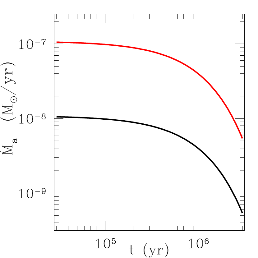
Figure 1.— Two different accretion histories considered in the models, following equation (1). Here and in all figures, a red line corresponds to the case with the highest accretion rate considered, while a black line is for the lowest accretion rate.

Figure 1 shows the evolution of the accretion rate, given by equation (1). In all of our models, we consider two different disk masses, $M_{D}=0.1$ and 0.01 $M_{\odot}$, to sample a range of accretion rates. We chose these two disk masses to represent a relatively high and low accretion rate, shown as a red and black solid line in figure 1, respectively. The true accretion histories of young stars are likely to be much more complex than equation (1), but this is not yet well-understood. The advantage of our approach is that it is simple, and it samples the wide range of accretion rates that is observed in optically visible accreting young stars (e.g., Hartmann et al., 1998; Sicilia-Aguilar et al., 2005; Natta et al., 2006).

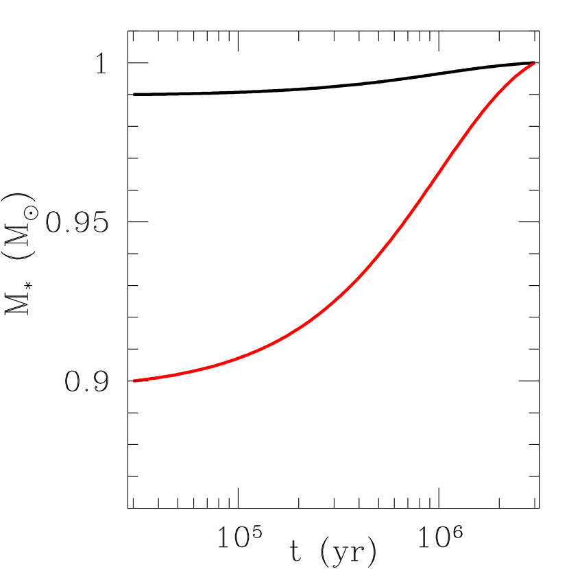
Figure 2.— Evolution of stellar mass, normalized to solar units, for the two different accretion histories considered. The red and black lines represent the high and low accretion rates, respectively. For each case, we chose the initial stellar mass such that the final mass would equal one solar mass.

Figure 2 shows the evolution of the stellar mass, which only depends on the prescribed accretion rate (eq. [1]) and an initial condition (at $t_{0}=3\times 10^{4}$ yr). For each of the two different accretion rates considered here, we set the initial stellar mass such that the final mass equals one solar mass. That is, the initial stellar mass equals one solar mass minus $M_{D}$, corresponding to 0.9 and 0.99 $M_{\odot}$ for the two cases.

2.2. Stellar Structure and Evolution

For the evolution of stellar radius, we adopt the simple treatment of CC93 and Yi (1994, 1995). This treatment models the structure of the star as a polytrope with an index of $n=3/2$ and assumes a constant photospheric temperature, $T_{e}$, during the Hayashi phase. The polytropic model results in a mean radius of gyration of $k^{2}=0.2$. The radiated, blackbody luminosity of the star is powered only by the release of gravitational potential energy, as the star contracts and accretes matter. The evolution of the stellar radius is then given by

$$\frac{dR_{*}}{dt}=2\frac{R_{*}}{M_{*}}\dot{M_{a}}-\frac{28\pi\sigma R_{*}^{4}T_{e}^{4}}{3GM_{*}^{2}},$$ (2)

where $G$ is Newton’s grativational constant and $\sigma$ is the Stefan-Boltzmann constant.

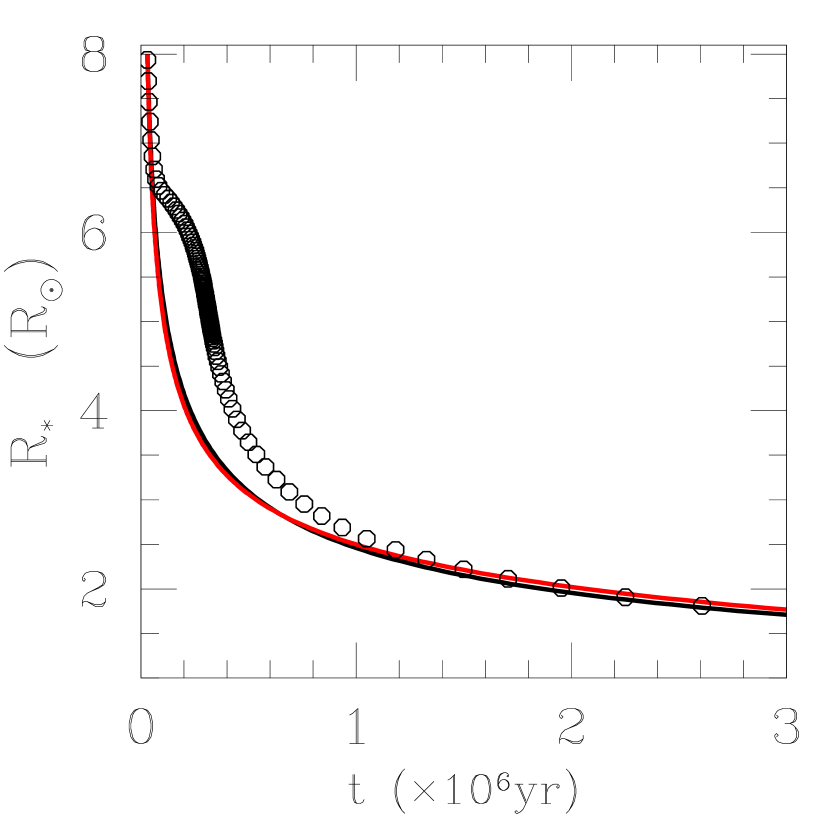
Figure 3.— Evolution of stellar radius normalized to solar units. The solid lines show solutions of equation (2), with the black and red lines corresponding to the low and high accretion rates (respectively) shown in figure 1 and discussed in section 2.1. For comparison, the circular symbols show the prediction of a more detailed model by Siess et al. (2000).

The black and red solid lines in figure 3 show the evolution of stellar radius with time, resulting from equations (1) and (2). In all of our models, we adopted an initial stellar radius of $8R_{\odot}$ and a photospheric temperature of $T_{e}=4280$ K. We chose these values in order to best match the radius evolution of a one solar mass star (with Z=0.02) predicted by the more sophisticated stellar model of Siess et al. (2000). Also, the chosen value of $T_{e}$ is within the narrow range of (nearly constant) Hayashi track temperatures exhibited by the Siess et al. (2000) model. For comparison, the circles in the figure show the Siess et al. (2000) model predictions.

It is clear from figure 3 that there is a “bump” in the Siess et al. radius evolution from $\sim 1$–$5\times 10^{5}$ yr that is not matched by our model. This is due to deuterium burning, which we neglect. Still, our simple treatment matches the Siess et al. model at the begining and end of the evolution, demonstrating that the overall evolution of stellar radius during this phase is dominated by the Kelvin-Helmholz contraction. Thus, our simple treatment is sufficient for the present purpose. Also, the treatment of equation (2) captures the effects of mass accretion, which is neglected in more sophisticated models (with the exception of Tout et al., 1999). To compute the evolution for a longer time, beyond the Hayashi track, would require the use of a more sophisticated stellar model, which we leave for future work.

2.3. Spin Evolution

Along with the prescription above for the evolution of the star’s mass, radius, and moment of inertia, the model also computes the angular momentum evolution. Assuming the star rotates as a solid body, the angular momentum equation can be expressed in terms of spin evolution,

$$\frac{d\Omega_{*}}{dt}=\frac{T_{*}}{I_{*}}-\Omega_{*}\left(\frac{\dot{M}_{a}}{M_{*}}+\frac{2}{R_{*}}\frac{dR_{*}}{dt}\right),$$ (3)

where $\Omega_{*}$ is the angular velocity of the star, and $T_{*}$ is the net torque on the star, discussed in section 2.4.

It is sometimes convenient to express the spin rate as a fraction of the breakup speed, defined as the Keplerian velocity at the star’s equator. This normalized spin rate is defined

$$f\equiv\Omega_{*}\sqrt{\frac{R_{*}^{3}}{GM_{*}}}.$$ (4)

In all of our models, we will consider two cases with different initial spin rates. The two cases have initial fractional spin rates of $f_{0}=0.3$ and 0.06, representing the two extremes of rapid and slow initial rotation. In all of our models, we enforce a maximum spin rate of $f=1$, since at this spin rate, some of the model assumptions (e.g., regarding the stellar structure) break down. As we show below, this limit is only reached in some of the most extreme models.

2.4. Star-Disk Interaction Torques

To calculate the torque on the star arising from accretion and the magnetic interaction between the star and disk, we follow the formulation of MP05. Here, we summarize the parts of that work that are relevant for our spin evolution model, and the reader will find details in that paper. This torque model follows several previous works (e.g., CC93; AC96; Ghosh & Lamb, 1978; Yi, 1994, 1995; Lovelace et al., 1995), but the primary advantage the MP05 formulation has for this work is that it includes the effects of varying magnetic coupling and magnectic connectedness between the star and disk.

2.4.1 Magnetic Field Prescription

The basic model is one-dimensional (in radius, $r$) and assumes the star has a rotation-axis-aligned dipolar magnetic field anchored into its surface, such that the magnetic field strength varies in the equatorial plane as

$$B_{z}=B_{*}\left(\frac{R_{*}}{r}\right)^{3},$$ (5)

where $B_{*}$ is the magnetic field strength at the equator and surface of the star. The surrounding accretion disk is assumed to be thin, so that the magnetic field has a negligible radial component along the disk surface.

The torque depends strongly upon the strength of the large-scale magnetic field $B_{*}$. Both disk locking and stellar wind spin-down models for T Tauri stars require global (dipolar) magnetic fields with surface strengths in the range of hundreds to thousands of Gauss. Observations of pre-main-sequence stars typically find field strenghts with a mean absolute value of $\sim 1$–3 kG (e.g., Basri et al., 1992; Johns-Krull, 2007; Johns-Krull et al., 2009), while the large-scale (global) fields of these stars appear to be at most several hundred Gauss (Safier, 1998; Johns-Krull et al., 1999a; Smirnov et al., 2004; Yang et al., 2007; Bouvier et al., 2007; Donati et al., 2007, 2008; Hussain et al., 2009). While this discrepancy means that the magnetic fields are complex (not simple dipoles), it is clear that these stars possess dynamically significant magnetic fields (Gregory et al., 2008). For the models presented here, we choose two values of the magnetic field strength, $B_{*}$ = 500 G and 2000 G, in addition to some cases with $B_{*}=0$, used for comparison.

Previous models for pre-main-sequence spin evolution (e.g., CC93; AC96; Yi, 1994, 1995) chose a prescription for the magnetic field that depends upon the stellar spin rate and stellar radius, as motivated by the expectations of a stellar dynamo. By contrast, for the models presented here, we choose to keep the magnetic field constant in time (a constant field was also considered in the works of Johns-Krull & Gafford, 2002 and Yi, 1994) for three reasons. First, observations of mean fields of T Tauri stars find a relatively constant field strength (Johns-Krull & Gafford, 2002; Johns-Krull, 2007), regardless of stellar age, radius, or spin rate. Measurements of large-scale field (Johns-Krull et al., 1999a; Smirnov et al., 2004; Yang et al., 2007; Bouvier et al., 2007; Donati et al., 2007, 2008; Hussain et al., 2009) are more rare, and there are not yet enough clear detections to look for trends. So a fixed field is consistent with observations. Second, the observed relationship between X-ray activity and spin rates of T Tauri stars (Stassun et al., 2004) suggests that they are primarily in the “saturated” or “supersaturated” regime (Johns-Krull, 2007), where solar-like stellar dynamo relationships are thought to break down. It is not yet clear how the global magnetic field behaves in this fully convective phase (Browning, 2008; Donati et al., 2008), but at this point, adopting a constant field strength seems appropriate. Finally, the main purpose of the present work is to demonstrate how the stellar spin rate is influenced by the magnetic coupling to the disk. Thus, it is also convenient for illustrative purposes to keep the field a fixed constant.

2.4.2 Magnetic Coupling to the Disk

The stellar magnetic field lines vertically threading the disk are imperfectly coupled to it. To be clear, throughout this paper, the term “coupling” refers to the extent to which the magnetic field is “frozen into” the disk material—that is, the effective magnetic diffusion in the disk. By contrast, the magnetic “connection” refers to the magnetic field loops that are attached both to the star and disk. MP05 showed how the strength of the coupling affects the amount of connected flux, and how this in turn affects the integrated torques.

The disk material rotates with Keplerian speed, which means that there is a singular location where the angular rotation rate of the disk equals that of the star, the corotation radius,

$$R_{\rm co}\equiv\left(\frac{GM_{*}}{\Omega_{*}^{2}}\right)^{1/3}=f^{-2/3}R_{*}.$$ (6)

Every location, except for $R_{\rm co}$, rotates at a different angular rate than the star. Thus, the magnetic field connected to the star and threading the disk will be twisted azimuthally (in the $\phi$-direction). It is assumed that the material above both the disk and star (the “corona”) is of sufficiently low density (high Alfvén speed) that the twisting of the magnetic field at the disk surface is equilibrated along the field line on a rapid timescale. Thus, the twisting of the magnetic field by the differential rotation between the star and disk imparts a torque, transferring angular momentum between the two.

The variable $\gamma(r)\equiv B_{\phi}/B_{z}$ quantifies the twist of the field at the surface of the disk at each radial location. This twisting occurs rapidly, on a stellar rotation timescale, so that a steady-state $\gamma(r)$ is simply determined by the balance between the differential rotation and the tendancy for the magnetic field to untwist by slipping (or reconnecting) azimuthally through the disk. This slipping rate depends on how well the magnetic field is coupled to the disk material.

To describe the coupling, MP05 adopted a dimensionless magnetic diffusivity parameter, which they assume to be constant throughout the disk,

$$\beta\equiv\frac{\eta_{t}}{hv_{k}},$$ (7)

where $\eta_{t}$ is the effective magnetic diffusivity, $h$ is the vertical thickness of the disk, and $v_{k}$ is the Keplerian rotation velocity. In other words, $\beta$ is the inverse of the effective magnetic Reynolds number of the star-disk interaction. A large value of $\beta$ corresponds to weak magnetic coupling (rapid field slipping through the disk), and a small value to strong coupling (slow slipping). The various models of star-disk interaction torques in the literature differ in their treatment of the magnetic field coupling, but all models adopt parameters that give similar results to MP05 with a value of $\beta$ of order unity. However, $\beta$ is a highly unknown parameter, and MP05 suggested that $\beta\lesssim 10^{-2}$ (i.e., large magnetic Reynolds number) may be more reasonable for accreting pre-main-sequence stars. In our models presented here, we consider $\beta=10^{-2}$ to represent the most realistic case, but we also show cases with $\beta=1$, for illustrative purposes.

2.4.3 Magnetic Connection State and $\gamma_{c}$

There is a dynamical limit to how strongly a dipolar magnetic field can be twisted azimuthally. As shown by several authors (Aly, 1985; Aly & Kuijpers, 1990; Lynden-Bell & Boily, 1994; Lovelace et al., 1995; Bardou & Heyvaerts, 1996; Agapitou & Papaloizou, 2000; Uzdensky et al., 2002), when the absolute value of the twist $\gamma$ exceeds a value near unity, the magnetic pressure force associated with $B_{\phi}$ pushes outward and leads to an opening of the dipole field loops. For practical purposes, this simply means that the star and disk are no longer causally linked, and no torques can be transmitted between the two. This does not mean the open field lines necessarily impart zero torque. Open field lines can, and likely do, transport some angular momentum from the star and/or disk (via winds). However, no angular momentum is exchanged between the star and disk along open field lines. In the present work, we consider only the torques arising in the star-disk interaction and thus neglect any torques that may arise from open field lines.

To take into account the opening of the field, the MP05 formulation includes a maximum for the absolute value of the twist, $\gamma_{c}$. In the regions of the disk where the twist is greater than this critical value, the model assumes that the magnetic field no longer connects the star to the disk. The torque on the star that would have arisen from those magnetic field lines is instead taken to be zero. MP05 showed that a value of $\gamma_{c}=\infty$ represents the classical assumption of a field that remains connected at all radii in the disk. To show the effect of the opening of the magnetic field in more realistic systems, a value of $\gamma_{c}=1$ is appropriate (Uzdensky et al., 2002).

Furthermore, MP05 showed that there exists a mode change in the magnetic connection between the star and disk, at a threshold value of the spin rate. Specifically, if

$$f<(1-\beta\gamma_{c})(\gamma_{c}\psi)^{-3/7},$$ (8)

where

$$\psi\equiv\frac{2B_{*}^{2}R_{*}^{5/2}}{\dot{M}_{a}\sqrt{GM_{*}}},$$ (9)

then the stellar magnetic field only connects to a small region near the inner edge of the disk. In this case, which they call “State 1,” no magnetic field connects the star to a radius in the disk that is larger than $R_{\rm co}$. This is significant, since in this state there exist no star-disk interaction torques that act to spin the star down (i.e., there are only spin-up torques). Alternatively, when equation (8) is not valid (for faster spin), the system is in “State 2,” characterized by a magnetic connection to the disk over a range of radii on either side of $R_{\rm co}$. In State 2, the star experiences both spin-up and spin-down torques. Figure 3 of MP05 illustrates these two magnetic connection states .

As evident in equation (8), magnetic connection State 1 only occurs for relatively extreme cases of slow spin rate, weak field, and/or high accretion rate. As it turns out, all of the models with non-zero $B_{*}$ presented in this paper remain in State 2 for the entire time simulated.

2.4.4 Truncation Radius and Accretion Torque

In the region of the disk at smaller radii than $R_{\rm co}$, the twist of the field is such that torques remove angular momentum from the disk (giving it to the star). If the magnetic field is strong enough, there will be a radius above the stellar surface at which these torques can extract all of the angular momentum of the material in the disk at that radius. Under these circumstances, the disk will be truncated, and accretion will proceed as a free-fall of material onto the star along the dipolar magnetic field lines.

In State 1 [eq. (8)], the location of the truncation radius is determined by

$${\rm(State\;1)}\;\;\;\;\;\;\;\;\;\;\;\;\;R_{t}=(\gamma_{c}\psi)^{2/7}R_{*}.$$ (10)

In State 2, the location of the truncation radius obeys

$${\rm(State\;2)}\;\;\;\;\left(\frac{R_{t}}{R_{\rm co}}\right)^{-7/2}\left[1-\left(\frac{R_{t}}{R_{\rm co}}\right)^{3/2}\right]=\frac{\beta}{\psi f^{7/3}},$$ (11)

which we solve for $R_{t}<R_{\rm co}$ using a Newton-Raphson method. In our models, for each timestep, we first use equation (8) to determine the magnetic connection state, then either equation (10) or (11) to find $R_{t}$. Finally, we check that $R_{t}$ is greater than $R_{*}$. If not, this means the magnetic field is not strong enough to truncate the disk above the stellar surface, and we reset $R_{t}$ to equal $R_{*}$.

The truncation of the disk is due to the stellar magnetic field extracting the angular momentum of disk material at a radius of $R_{t}$. Thus, the truncation of the disk and subsequent accretion of material adds angular momentum to the star at a rate equal to

$$T_{a}=\dot{M}_{a}\sqrt{GM_{*}R_{t}},$$ (12)

which is referred to as the “accretion torque”. Note that, although equation (12) does not explicitly contain a dependence on the magnetic field strength, the magnetic field is central to the determination of $R_{t}$ (as long as $R_{t}>R_{*}$). Furthermore, when $R_{t}>R_{*}$, material falling onto the star transfers the bulk of its angular momentum to the magnetic field before the material reaches the stellar surface (e.g., Romanova et al., 2002; Long et al., 2005). Thus, as long as $R_{t}>R_{*}$, the torque of equation (12) is experienced by the star as a magnetic torque, although we still refer to this as the “accretion torque” to distinguish it from the component of the torque described in section 2.4.5.

2.4.5 Magnetic Torque

In addition to the accretion torque, if the system is in State 2, the magnetic connection over a range of radii in the disk transports angular momentum between the star and the disk. In this case

$${\rm(State\;2)}\;\;\;\;T_{m}=\frac{B_{*}^{2}R_{*}^{6}}{3\beta R_{\rm co}^{3}}[2(1+\beta\gamma_{c})^{-1}-(1+\beta\gamma_{c})^{-2}$$

$$-2(R_{\rm co}/R_{t})^{3/2}+(R_{\rm co}/R_{t})^{3}],\;\;\;\;\;$$ (13)

is the net torque felt by the star from both spin-up and spin-down components. We refer to this as the “magnetic torque.” If the system is in State 1, the magnetic field does not connect to a significant range of radii in the disk, so we set

$${\rm(State\;1)}\;\;\;\;\;\;\;\;T_{m}=0.$$ (14)

As discussed in MP05, we assume that the disk will be capable of transporting away any angular momentum that it receives from the star (i.e., from negative torques in eq. [2.4.5]). For example, the disk may restructure itself in response to external torques (e.g., Rappaport et al., 2004) in such a way as to increase the effectiveness of viscous or turbulent angular momentum transport.

2.4.6 Total Torque and Equilibrium Spin Rate

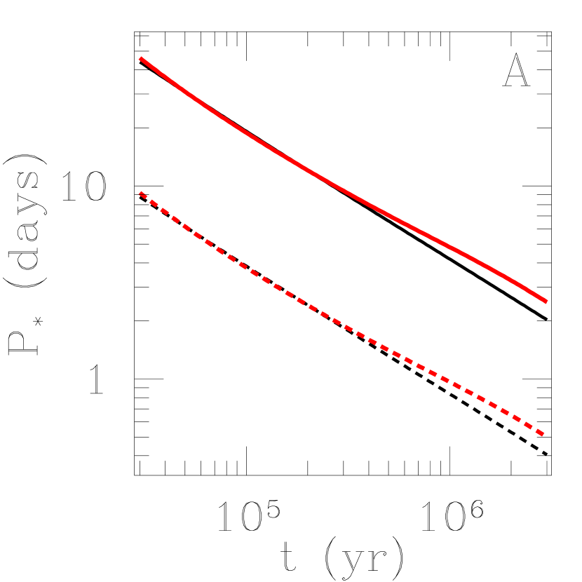
Figure 4.— Evolution of spin period (panel a) and spin rate expressed as a fraction of the breakup rate (panel b) for a star with no external torques ($T_{*}=0$). The four cases shown represent the two choices of accretion history and the two initial spin rates. The red and black lines correspond to the high and low accretion cases, respectively. The solid and dashed lines correspond to models with an initial spin rate of 0.06 and 0.3 times the breakup rate, respectively.

The total torque on the star is the sum of the accretion and magnetic torques,

$$T_{*}=T_{a}+T_{m},$$ (15)

and we neglect any other torques that may be present (e.g., from a stellar wind). The total torque can be either postive or negative, depending on the balance between spin-up torques (due to the trucation of the disk and to magnetic field lines that are azimuthally twisted in a direction that leads the rotation of the star) and spin-down torques (due to magnetic field lines that are twisted in a direction that lags the rotation of the star).

For any given system, there is a particular stellar spin rate at which the net torque will equal zero ($T_{*}=0$). This is called the equilibrium spin rate, and the torque always acts to change the stellar spin in a direction toward this equilibrium. As indicated in equation (3), the spin also changes in response to changes in stellar radius and mass, and in general to changes in the moment of inertia. If the contribution from the torque is large compared to that from changes in the moment of inertia, the stellar spin will evolve asymptotically toward the equilibrium rate.

This general idea provides the theoretical underpinning for the idea of disk locking (Ghosh & Lamb, 1978; Camenzind, 1990; Königl, 1991; Edwards et al., 1993; Shu et al., 1994), which holds that the stellar spin rate is determined by the current conditions in the star-disk interaction and independent of any initial conditions. MP05 described the method of computing the stellar spin rate in this hypothetical equilibrium state for their torque formulation, which uses equations (23)–(27) of that work. In presenting our results below, we compare the actual spin rates to the equilibrium values to gain insight into these systems.

2.5. Numerical Method

The coupled equations (1), (2), and (3) describe the evolution of the system. We wrote a computational code that solves these simultaneously, using the fourth-order Runge-Kutta scheme of Press et al. (1994), starting from $t_{0}=3\times 10^{4}$ yr and ending at 3 Myr. For computational efficiency and numerical stability, we use a dynamic timestep. At each step, we compute the next timestep by requiring that none of the three main variables, $\Omega_{*}$, $R_{*}$, $M_{*}$, change by more than 1% per step. This gives results converged to three significant figures and typically requires a few hundred timesteps for the entire evolution.

In order to compute the torque at each timestep, the code first solves equation (8) to determine the magnetic connection state of the system. Then, depending on the state, the code solves either equation (10) or (11) to determine the disk truncation radius. We enforce a minimum value of $R_{t}=R_{*}$. Finally, the code calculates the accretion torque using equation (12) and the magnetic torque using either equation (2.4.5) or (14). The torque is assumed to be constant during each timestep. We also enforce a maximum on the spin rate, corresponding to $f=1$ (see §2.3).

3. Results

Table 1Model Parameters

Case	$\gamma_{c}$	$\beta$	$B_{*}$ (Gauss)	$M_{D}/M_{\odot}$	$f_{0}$	Figure
$T_{*}=0$	$\cdots$	$\cdots$	$\cdots$	0.01, 0.1	0.06, 0.3	4
$B_{*}=0$	$\cdots$	$\cdots$	0	0.01, 0.1	0.06, 0.3	5
O1	1	0.01	500	0.01, 0.1	0.06, 0.3	6
O2	1	0.01	2000	0.01, 0.1	0.06, 0.3	7
O3	1	1	2000	0.01, 0.1	0.06, 0.3	8
C1	$\infty$	1	500	0.01, 0.1	0.06, 0.3	9
C2	$\infty$	1	2000	0.01, 0.1	0.06, 0.3	10

This section contains results from several models. Table 1 lists the parameters for all cases, in order of their presentation and grouped by the figures in which the results appear. All models have the same initial stellar radius ($8R_{\odot}$) and effective temperature ($T_{e}=4280$ K; see fig. 3 and §2.2). Also, all models end with a mass of $M_{\odot}$, so that the initial mass depends on the accretion rate (see §2.1). For each case in table 1, we ran four models, one for each combination of two different initial spin rates (see §2.3) and two different mass accretion rates (see §2.1). These parameters are intended to represent a range that is appropriate for accreting T Tauri stars.

Section 3.1 includes two simplified cases with no magnetic fields: one in which $T_{*}=0$, so that there is no star-disk interaction; and one in which $B_{*}=0$ so that there are no magnetic effects, just disk accretion. Section 3.2 contains the main results, models that include magnetic fields with realistic field line opening ($\gamma_{c}=1$) and different values of $\beta$, for two different field strengths. For comparison, and as a verification of our model and computations, the appendix contains results for cases with the classical assumption of a fully closed magnetic field ($\gamma_{c}=\infty$) and $\beta=1$.

3.1. $T_{*}=0$ and $B_{*}=0$ Cases

Figure 5.— Results for $B_{*}=0$. Panel (a) and (b) show the same quantities as figure 4. The solid, dashed, red, and black lines in all panels have the same meaning as in figure 4. Panel (c) shows the net torque on the star for each case. In this panel, the dashed and solid lines of a given color lie on top of each other, since the spin rate does not affect the torque when $B_{*}=0$. The horizontal dotted line indicates $T_{*}=0$ for clarity. Panel (d) shows the location of the truncation radius ($R_{t}$, thick lines) and the corotation radius ($R_{\rm co}$, thin lines; eq. [6]), in units of the stellar radius. Here, $R_{t}=R_{*}$ for all models, since there is no magnetic field to truncate the disk above the stellar surface.

To begin, it is useful to examine a few simplified cases. The main goal is to understand individually how the stellar contraction and accretion alone affects the spin evolution, before adding the effects of magnetic fields. We will consider two cases here: one in which the net torque on the star is forced to be zero; and one in which there are no magnetic fields, so that the only torque on the star is due to the accretion of material from the disk.

Figure 4 shows the evolution of stellar spin for the case of zero torque ($T_{*}=0$ in eq. [3]). The figure shows both the spin period, $P_{*}=2\pi/\Omega_{*}$, as well as the spin rate expressed as a fraction of breakup speed (eq. [4]), as a function of time. In this figure and in each subsequent figure, we show four different simulations, representing all combinations of two different accretion rates and two different initial spin rates. The red (black) colored lines correspond to the highest (lowest) accretion rate considered (see §2.1 and figure 1). The solid (dashed) lines correspond to the slow (fast) initial spins considered (see §2.3).

The spin evolution of the stars in figure 4 is due to contraction and the accretion of mass containing no angular momentum. After the initial time of $3\times 10^{4}$ yr, the cases with higher accretion rates (red lines) spin somewhat more slowly than the cases with lower accretion rates. This is because the stars in the high accretion cases are gaining more mass, while conserving their angular momentum. Still, this effect is relatively minor, and it is clear that the spin evolution is dominated by the change in stellar radius. Specifically, the contraction from the beginning to the end of the evolution (see figure 3), leads to a change in spin period by a factor of approximately 20, and a change in $f$ by a factor of approximately 2.

Next, we consider the case where angular momentum is added to the star from the accretion of disk material. Since the disk is assumed to be in Keplerian orbit, it has high specific angular momentum relative to the star. In the simplified case where the star has no magnetic field, the disk material will extend all the way to the surface of the star, forming a boundary layer (Lynden-Bell & Pringle, 1974). The torque on the star from the boundary layer is given by equation (12), with $R_{t}=R_{*}$. This behavior is captured automatically in our model by setting $B_{*}=0$.

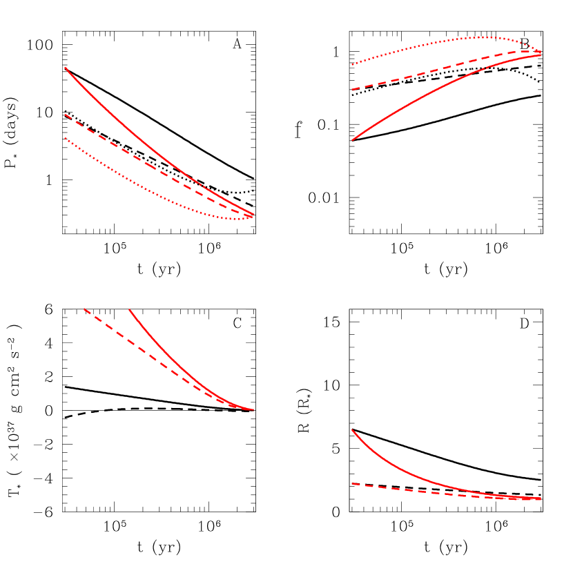
Figure 6.— Results for $B_{*}=500$ G, $\gamma_{c}=1$, and $\beta=0.01$, in the same format as figure 5. In panels (a) and (b), the dotted red and black lines show the equilibrium value (§2.4.6) for the high and low accretion rates, respectively. In panel (d), the thin and thick lines of a given color and type are indistinguishable, since $R_{t}$ is very close to $R_{\rm co}$ in all four cases.

Figure 5 shows this case for the two different accretion rates and two different intiial spin rates. In addition to the evolution of stellar spin (panels a and b), the figure shows the net torque on the star (panel c) and the location of the disk truncation radius and the corotation radius (panel d). Panel (c) indicates that the torque on the star is always positive (adding angular momentum to the star). The torque does not depend on the spin rate of the star but depends most strongly on the accretion rate (eq. [12]). Thick lines in panel (d) all overlap, indicating that the disk extends all the way to the stellar surface ($R_{t}=R_{*}$, as expected) in all of these cases. The thin lines in panel d show how the corotation radius (eq. [6]) changes with spin rate.

It is clear from figure 5 how the accretion torque influences the spin evolution of the star. For the lowest accretion rate considered, after 3 Myr, the star spins about 10% to 50% faster than in the $T_{*}=0$ case (fig. 4). But for the highest accretion rate considered, the stars spin much faster. The most extreme case, with a high accretion rate and fast initial spin (dashed red line), reached the $f=1$ limit enforced by our model (see §2.3) in approximately 1.5 Myr. In the case with the slowest initial spin and lowest accretion rate, the spin period is 1–2 days during the last few Myr. But the other three cases have spin periods shorter than one day during that time. In order to explain the observed spin periods of several days, for the range of accretion rates considered here, these stars must experience significant spin down torques. The next subsection presents cases that include the additional effects of torques that arise in the magnetic star-disk interaction.

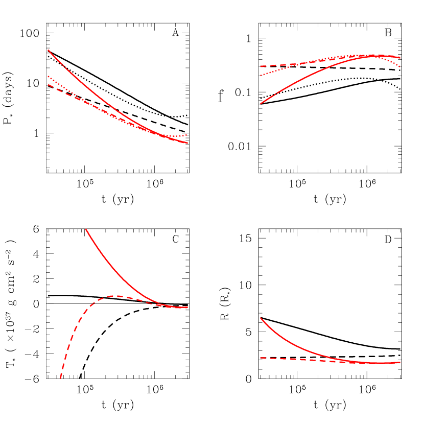
Figure 7.— Results for $B_{*}=2000$ G, $\gamma_{c}=1$, and $\beta=0.01$, in the same format as figure 6.

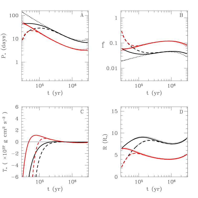
Figure 8.— Results for $B_{*}=2000$ G, $\gamma_{c}=1$, and $\beta=1$, in the same format as figure 6.

3.2. Effect of the Magnetic Star-Disk Interaction

The results in the previous section demonstrate how the spins of accreting stars are expected to evolve in the absence of magnetic effects. In this section, we include the magnetic torques that arise from the magnetic star-disk interaction. The torque calculation follows MP05 (described in §2.4), and we adopt $\gamma_{c}=1$ in order to include the effect of the opening of the field that is expected to arise due to the differential rotation between the star and disk.

Figure 6 shows the results for cases with a dipole field strength of $B_{*}=500$ G at the equator of the star, and $\beta=0.01$. This field strength is similar to the strongest yet measured dipole field on an accreting young star, 600 G for BP Tau (Donati et al., 2008). This value for $\beta$ was suggested by MP05 to best represent real systems (see §2.4.2). The four models are shown in the same format as figure 5 and represent case O1 in table 1. A comparison of the upper panels of figures 5 and 6 reveals that the magnetic star-disk interaction has very little influence on the spin evolution, in this case. In most models, the presence of a 500 G dipole field results in spin rates that are 10-30% faster at an age of 3 Myr than the $B_{*}=0$ case. Only the model with low accretion rate and fast initial spin (black, dashed line) spins more slowly (by $\sim 10$%) than the non-magnetic case.

Panel (d) of figure 6 indicates that in all models, the disk is truncated very close to the corotation radius (the lines for $R_{t}$ and $R_{\rm co}$ are indistinguishable). Thus, the 500 G dipole is strong enough to truncate the disk, leading to magnetospheric accretion, in spite of the fact that the stellar spin evolution is not largely affected.

The red and black dotted lines in panels (a) and (b) of figure 6 represent the hypothetical equilibrium (disk locked) spin rate (see §2.4.6) for the two different accretion rates considered. It is clear that the three models that spin faster than the non-magnetic case are all spinning more slowly than their corresponding equilibrium rate. This means that the net torque on these stars is positive (acting to spin up the star). Furthermore, a comparison of panels (c) in figures 5 and 6 indicates that these three models have a larger net torque in the magnetized (O1) case. This explains why these models end up spinning slightly faster than the non-magnetized case. The model with low accretion rate and fast initial spin (black, dashed line) evolves near the equilibrium rate, resulting in a near zero torque in panel (c). However, this is simply due to a coincidence of the initial condition with the equilibrium rate, since the torque is not strong enouth to maintain equilibrium within million-year timescales.

In the disk-locking scenario, the magnetic star-disk interaction torques are strong enough to keep the spins near their equilibrium rate. The case with $B_{*}=500$ G presented in the appendix (C1, figure 9), where field line opening is ignored, does approximately follow the expectations of disk locking. However, this is clearly not true for the O1 case (figure 6), since the spins of all four models at all times depend upon the choice of initial spin rate. The main result of case O1 is that, when considering the opening of the field and strong magnetic coupling, a dipole magnetic field strength of 500 G is not strong enough to significantly influence the spin evolution of one solar mass accreting pre-main-sequence stars.

Figure 7 shows the results for the O2 case, which is the same as O1, except that the magnetic field is much stronger ($B_{*}=2000$ G). In the O2 case, the magnetic star-disk interaction has more of an influence on the spin evolution. By comparing the top panels of figures 6 and 7, it is clear that all models are spinning more slowly in the O2 case.

The spin rates of the two models with the high accretion rate (red, solid and red, dashed lines) converge toward the equilibrium value at an age of $\sim 1$ Myr. Thus, these models approach the disk locked state, and the initial condition is “erased” at that time. The same is not true for the models with the low accretion rate (black, solid and black, dashed lines), since the spin rate after 3 Myr still depends upon the intial spin rate for those models.

The O2 case is significantly different than the case with $B_{*}=2000$ G presented in the appendix (C2, figure 10), which ignores field line opening. By comparison, the disk locking in the O2, high-accretion models is marginal and only happens after $\sim 1$ Myr, which is approaching the lifetime of disks. Furthermore, it is important to note that the rotation periods of all models in the O2 case are less than $\sim 3$ days in the age range of 1–3 Myr. This is consistent only with the fastest rotators in the observed spin distributions (see §1).

Thus far, we have considered $\beta=0.01$, since this was suggested by MP05. However, MP05 showed that the spin-down torque felt by the star is the strongest for a magnetic coupling strength of $\beta=1$. This is indeed a highly diffusive situation, as this means that a magnetic field line that is tilted by 45^∘ will slip through the disk at a speed equal to the Keplerian speed (see MP05). Although this is unexpectedly diffusive for an astrophysical plasma, the correct value of $\beta$ for these systems is highly uncertain. Thus, it is instructive to look at this case, which will have the most extreme effect on the stellar spins.

Figure 8 shows the results of this extreme case, with $\beta=1$ and $B_{*}=2000$ G (case O3). It is clear that, in this case, the star-disk interaction completely dominates the spin evolution of the stars. The spin rates converge toward their respective equilibrium values in 1–3$\times 10^{5}$ yr. Subsequent evolution closely follows the equilibria, consistent with the disk locking scenario. The spin periods are in the range of 3–10 days for ages of 1–3 Myr. It is evident from panel (d) that the disk truncation radii are close to the corotation radii, but not so close that the lines overlap. This difference from the previous 2 cases is due primarily to the much higher magnetic diffusion rate in the O3 case.

4. Discussion and Conclusions

The star-disk interaction model of MP05 includes the effects of the field opening expected to arise from star-disk differential rotation ($\gamma_{c}=1$), as well as the effects of magnetic coupling, parameterized by $\beta$. Based essentially upon the idea that the disk likely exists in a state of high magnetic Reynolds number, MP05 argued that a value of $\beta=0.01$ is appropriate for real systems. In the present work, we have extended the MP05 torque model into the time domain, in order to explore the consequences of magnetic star-disk coupling and connectedness on the evolution of stellar spins.

To this end, we developed a stellar spin evolution model (§2). The model follows an accreting, one solar mass star during the Hayashi phase (from $3\times 10^{4}$ yr to $3$ Myr) and considers the torques expected to arise from the magnetic star-disk interaction. The primary goals of this work were to examine the role of disk locking and to determine if the star-disk interaction torques alone are sufficient to explain the observed range of spin rates. In developing our torque and spin-evolution model, we have adopted many of the same assumptions as the disk-locking models in the literature, except that the MP05 torque formulation includes the effect of the opening of the magnetic field. Thus, while there are inherant uncertainties associated with the adoption of many of these assumptions, our results serve best to highlight the effect of field opening relative to previous results in the literature.

Given the expectation that $\gamma_{c}=1$ and $\beta=0.01$ best-represents the conditions in real systems, and for a range of accretion rates and field strengths appropriate for T Tauri stars, the two main conclusions of the present work are as follows:

1. The models presented in figures 6 and 7 exhibit spin periods ranging from 3 days to less than 1/3 day, in the age range of 1–3 Myr (see §3.2). These are consistent only with the fastest rotators in the observed spin period distribution, which is significantly populated from approximately 1–10 days (see §1). It is apparent that the torque arising from the magnetic connection between the star and disk is not sufficient to explain the relatively slowly spinning, young stars.

2. Furthermore, the stars in these models are generally not in spin equilibrium (with a net zero torque), and the spin rate at all times depends upon the initial spin rate (see §3.2). Only the models with the strongest field strength and highest accretion rate neared their equilibrium spin rate in $\sim 1$ Myr (see figure 7). However, this equilibrium had a relatively short spin period of less than a day. It is apparent that disk locking does not play a strong role, except possibly for the most rapid rotators.

Note that the term “disk locking” generally refers to the idea that the angular spin rate of the star is nearly equal to that of the inner edge of the disk (i.e., $R_{t}\approx R_{\rm co}$). In our magnetic models, this condition was always true. In fact, the truncation radius was nearest to the corotation radius in the models that were furthest from spin equilibrium (e.g., compare panel (d) in figures 6 and 9). Thus, these stars do have an angular spin rate that is very close to that of the disk inner edge, although it is not appropriate to think of these systems as being “locked” to any particular spin rate. Instead, this is a consequence of how the disk is truncated. When the magnetic coupling in the disk is strong (small $\beta$), the disk will generally be truncated close to the corotation radius (in State 2; see §2.4.4). But, the condition that $R_{t}\approx R_{\rm co}$ does not necessarily mean that the star experiences a net zero torque.

In order to explain the existence of slowly rotating young stars, it is necessary to consider other possibilities. Since the magnetic torques depend strongly on the magnetic field strength, it is tempting to suggest that a stronger magnetic field may solve the problem. Using our model, we find that (for $\beta=0.01$) a dipole field strength of $B_{*}=10^{4}$ G is required to maintain spin periods consistent with the slow rotators. However, no T Tauri star has been found to have surface field strengths greater than 3 kG (Johns-Krull, 2007), and the global (dipole) fields are generally even weaker (e.g., Safier, 1998; Bouvier et al., 2007; Donati et al., 2007, 2008). Given the relatively small number of stars for which there are magnetic field measurements, the present situation could be improved by more and improved observations of the global field strength and geometry.

Since the models presented in section 3.2 with weak magnetic coupling (figure 8) exhibit slow spins, it is also appropriate to consider the possibility that real systems have weak coupling. As discussed above, the conditions that are expected to best represent young star-disk systems from “first principles” suggest values of $\beta=0.01$. However, $\beta$ is a highly uncertain parameter because the physics of magnetic coupling is not well understood, nor are the conditions that influence the coupling (e.g., the ionization fraction of disk gas, turbulence levels in the disk, or magnetic reconnection rates). In order for magnetic coupling to explain the slow rotators, the coupling strength must not be very different (neither larger nor smaller) than $\beta=1$, since MP05 showed that the maximum spin-down torque occurs for a $\beta$ of unity. The condition that $\beta\approx 1$ seems to require some fine-tuning, which makes this possiblity even more difficult to justify at present.

Therefore, it appears necessary to consider effects that are alternative or additional to the magnetic torques arising from the star-disk connection. Real systems seem to be variable on all timescales (e.g., Hartmann, 1997), and we have neglected variability here. It may be possible, for example, that short timescale (e.g., $\lesssim 10^{4}$ yr), large-magnitude variations of the accretion rate are important for the stellar mass and angular momentum evolution (e.g., Popham, 1996). Finally, it is necessary to consider the angular momentum loss from pre-main-sequence stellar winds (see §1). The idea that stellar winds may be important during the accretion phase is well-supported (e.g., Decampli, 1981; Hartmann et al., 1982; Kwan & Tademaru, 1988; Hartmann et al., 1990; Fendt et al., 1995; Fendt & Camenzind, 1996; Safier, 1998; Bogovalov & Tsinganos, 2001; Sauty et al., 2002; Edwards et al., 2003, 2006; Dupree et al., 2005; Meliani et al., 2006; Kurosawa et al., 2006; Kwan et al., 2007; Fendt, 2009). Stellar winds may be powered by the accretion process itself (Tout & Pringle, 1992; Cranmer, 2008) and be the key driver of angular momentum loss (Hartmann & MacGregor, 1982; Mestel, 1984; Hartmann & Stauffer, 1989; Paatz & Camenzind, 1996; Matt & Pudritz, 2005a, 2008a, 2008b).

Some recent magnetohydrodynamic (MHD) simulations of rapidly rotating stars (e.g., Romanova et al., 2005, 2009) exhibit a type of “propeller” regime in which intermittent accretion occurs on typical timescales of several orbits of the inner disk, while most of the would-be accreting material is instead launched into a wind. For the calculations in the present work, the torque represents that which is averaged over a calculation timestep. Our timesteps range from approximately 400 years (at the earliest times) to $\sim 10^{5}$ yrs. While some of the simulations in the work cited above have been run for thousands of dynamical times, this is still orders of magnitude shorter than the typical timestep in the present work. It is not clear whether the torque formulation we adopted accurately describes the time-average behavior of the accretion and closed field region in the propeller regime simulations. In addition, while these MHD simulations reliably demonstrate many of the complexities and sometimes episodic nature of the magnetic star-disk interaction, when considering the long-term evolution of the star and disk, it is not yet clear whether the duration of the episodic (e.g., propeller) regime is significant for the overall spin evolution of young stars. However, the MHD simulations such as those cited above often exhibit significant outflows and torques arising from open magnetic field regions. In this respect, our result that the torques arising only from closed field regions are not sufficient to significantly spin-down the star, agrees with the simulations.

It is clear that the opening of field lines is an important effect, since including this in the models indicates considerably different physics at work than the closed field models, when comparing to the same observational data. In future work, we will extend the present analysis to include the angular momentum loss from accretion-powered stellar winds.

Appendix A Cases With Closed Magnetic Field ($\gamma_{c}=\infty$)

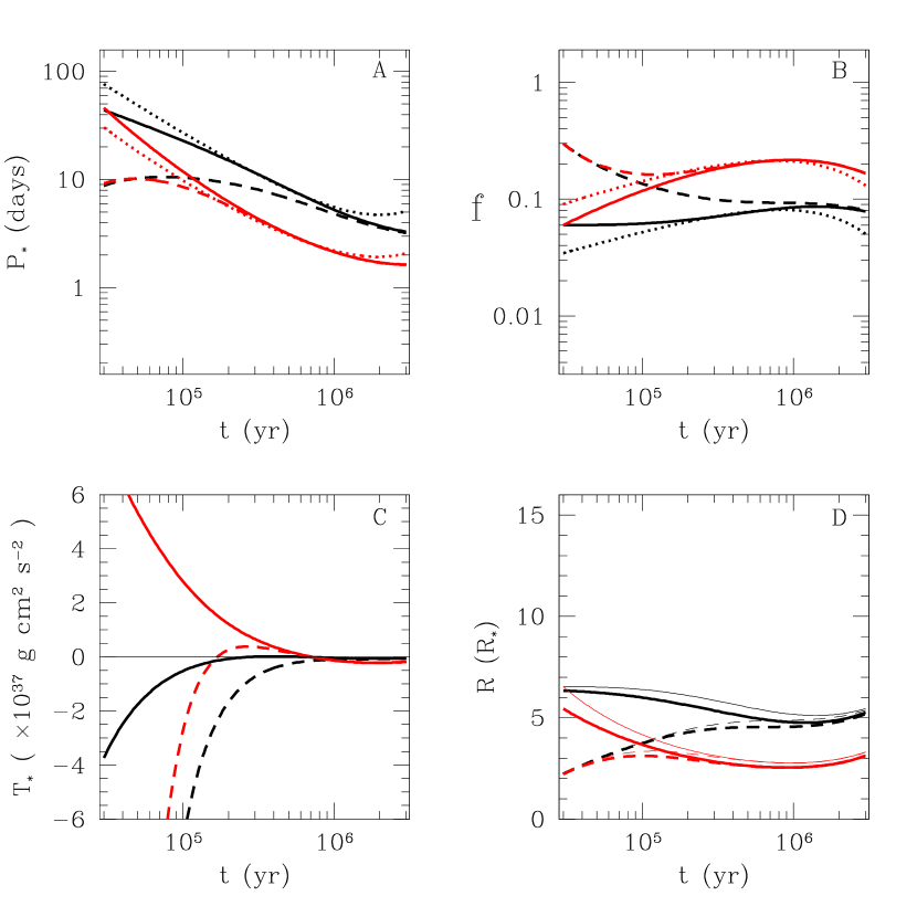
Figure 9.— Results for $B_{*}=500$ G, $\gamma_{c}=\infty$, and $\beta=1$, in the same format as figure 6.

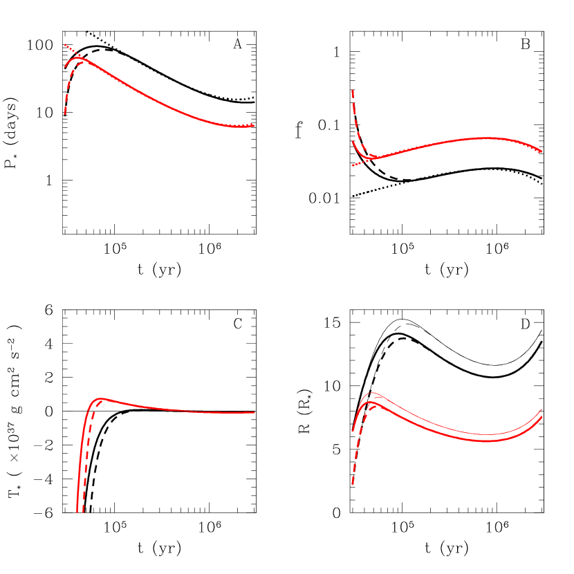
Figure 10.— Results for $B_{*}=2000$ G, $\gamma_{c}=\infty$, and $\beta=1$, in the same format as figure 6.

In order to demonstrate that our model and code reproduces the results of the classical models, and for comparison to the cases presented in section 3, here we present cases with $\gamma_{c}=\infty$. With the MP05 torque formulation, this value of $\gamma_{c}$ keeps the magnetic field connected everywhere to the disk, regardless of how twisted the field becomes. This well-represents the classical Ghosh & Lamb (1978) model, and results in stronger spin-down torques on the star. Most star-disk interaction and disk-locking models follow the Ghosh & Lamb model and assume a magnetic coupling strength that is equivalent (within $\sim$20%) to a value of $\beta=1$. Thus, we adopt this value of $\beta$ here.

In table 1, the two cases presented here are labeled C1 and C2, which have $B_{*}=500$ G and $B_{*}=2000$ G, respectively. Figures 9 and 10 show results from these two cases, where the line styles and colors have the same meaning as in figure 6. The spin evolution of all models in both figures is dominated by the magnetic interaction between the star and disk. For the $B_{*}=500$ G case (figure 9), the spin rates converge toward their equilibrium values in $2\times 10^{5}$ and $10^{6}$ yr for the cases with high and low accretion rates, respectively. For the $B_{*}=2000$ G case (figure 10), convergence occurs for all models within $\sim 10^{5}$ yr. Thus, when the magnetic field is not allowed to open as expected, the evolution follows closely with the expectations of the disk locking scenario.

As in all other magnetic models presented in this paper, the disk truncation radii remain near, although slightly inside, the corotation radii. However, in these cases with $\gamma_{c}=\infty$, $R_{t}$ is generally further away from $R_{\rm co}$ than in the cases presented in section 3. This is a consequence of the stronger spin-down torques and higher value of $\beta$ for the models of this section.

Examination of figures 9 and 10 reveals that the spin rates are slower when the magnetic field strength is higher or the accretion rate is lower. Under the conditions of disk locking, the angular spin rate of the star is proportional to $\dot{M}_{a}^{3/7}B_{*}^{-6/7}$, which is exhibited in the models presented here. Furthermore, the spin periods of all the models are in the range of 1.5–20 days during the ages of 1–3 Myr. These values are consistent with the range of observed spin periods (see §1), and this has been the primary physical justification for the disk-locking picture being applied to young stars.

The models presented in this section produce very similar quantitative results to the spin evolution models of Yi (1994, 1995) and AC96. The main differences between all of these works is the treatment of the magnetic field and accretion rates. In particular, other works considered a magnetic field strength that evolved with stellar spin rate and stellar radius. Here, we have assumed a constant surface magnetic field strength. Our assumption results in different behavior from those models, particularly at times earlier than $\sim 1$ Myr. At these younger ages, the stars have relatively large radii, and the assumption of a constant surface field strength means that the total magnetic energy in the field (proportional to $B_{*}^{2}R_{*}^{3}$) is larger. This is the main reason that the equilibrium spin rates are slowest at earlier times, in our models. The models of Yi (1994, 1995) and AC96 exhibit spin periods that are more nearly constant in time, due the different prescription of the field. Still, when our results and those of Yi (1994, 1995) and AC96 are scaled according to the torque theory to similar values of accretion rates and field strengths, the results are quantitatively consistent.

The spin evolution model of CC93 is somewhat different from other works. The assumptions in that work lead to a magnetic coupling that is significantly stronger than in Yi (1994, 1995), AC96, and most other models. We have determined that we get similar results to CC93 for models with $\gamma_{c}=\infty$ and a coupling strength of $\beta=0.05$. This relatively strong coupling leads to a large azimuthal twisting of the magnetic field. This, together with the requirement that the magnetic field remain closed, leads to very strong spin-down torques on the star. For this reason, the CC93 model predicts slower equilibrium spins than other models for a given field strength (e.g., see Johns-Krull et al., 1999b; Johns-Krull, 2007). However, as shown in section 3, when the opening of the field is properly taken into account, the spin-down torques are weaker, and the magnitude of this effect is larger for cases with strong magnetic coupling (as in the CC93 model).

References

- Agapitou & Papaloizou (2000) Agapitou, V. & Papaloizou, J. C. B. 2000, MNRAS, 317, 273
- Aly (1985) Aly, J. J. 1985, A&A, 143, 19
- Aly & Kuijpers (1990) Aly, J. J. & Kuijpers, J. 1990, A&A, 227, 473
- Armitage & Clarke (1996) Armitage, P. J. & Clarke, C. J. 1996, MNRAS, 280, 458
- Attridge & Herbst (1992) Attridge, J. M. & Herbst, W. 1992, ApJ, 398, L61
- Bardou & Heyvaerts (1996) Bardou, A. & Heyvaerts, J. 1996, A&A, 307, 1009
- Basri et al. (1992) Basri, G., Marcy, G. W., & Valenti, J. A. 1992, ApJ, 390, 622
- Bessolaz et al. (2008) Bessolaz, N., Zanni, C., Ferreira, J., Keppens, R., & Bouvier, J. 2008, A&A, 478, 155
- Bogovalov & Tsinganos (2001) Bogovalov, S. & Tsinganos, K. 2001, MNRAS, 325, 249
- Bouvier et al. (2007) Bouvier, J., Alencar, S. H. P., Harries, T. J., Johns-Krull, C. M., & Romanova, M. M. 2007, in Protostars and Planets V, ed. B. Reipurth, D. Jewitt, & K. Keil, 479–494
- Bouvier et al. (1997) Bouvier, J., Forestini, M., & Allain, S. 1997, A&A, 326, 1023
- Browning (2008) Browning, M. K. 2008, ApJ, 676, 1262
- Camenzind (1990) Camenzind, M. 1990, in Reviews in Modern Astronomy, ed. G. Klare, 234–265
- Cameron & Campbell (1993) Cameron, A. C. & Campbell, C. G. 1993, A&A, 274, 309
- Choi & Herbst (1996) Choi, P. I. & Herbst, W. 1996, AJ, 111, 283
- Cieza & Baliber (2007) Cieza, L. & Baliber, N. 2007, ApJ, 671, 605
- Covey et al. (2005) Covey, K. R., Greene, T. P., Doppmann, G. W., & Lada, C. J. 2005, AJ, 129, 2765
- Cranmer (2008) Cranmer, S. R. 2008, ApJ, 689, 316
- de la Reza & Pinzón (2004) de la Reza, R. & Pinzón, G. 2004, AJ, 128, 1812
- Decampli (1981) Decampli, W. M. 1981, ApJ, 244, 124
- Donati et al. (2007) Donati, J.-F., Jardine, M. M., Gregory, S. G., Petit, P., Bouvier, J., Dougados, C., Ménard, F., Cameron, A. C., Harries, T. J., Jeffers, S. V., & Paletou, F. 2007, MNRAS, 380, 1297
- Donati et al. (2008) Donati, J.-F., Jardine, M. M., Gregory, S. G., Petit, P., Paletou, F., Bouvier, J., Dougados, C., Ménard, F., Cameron, A. C., Harries, T. J., Hussain, G. A. J., Unruh, Y., Morin, J., Marsden, S. C., Manset, N., Aurière, M., Catala, C., & Alecian, E. 2008, MNRAS, 386, 1234
- Dupree et al. (2005) Dupree, A. K., Brickhouse, N. S., Smith, G. H., & Strader, J. 2005, ApJ, 625, L131
- Edwards et al. (2006) Edwards, S., Fischer, W., Hillenbrand, L., & Kwan, J. 2006, ApJ, 646, 319
- Edwards et al. (2003) Edwards, S., Fischer, W., Kwan, J., Hillenbrand, L., & Dupree, A. K. 2003, ApJ, 599, L41
- Edwards et al. (1993) Edwards, S., Strom, S. E., Hartigan, P., Strom, K. M., Hillenbrand, L. A., Herbst, W., Attridge, J., Merrill, K. M., Probst, R., & Gatley, I. 1993, AJ, 106, 372
- Fendt (2009) Fendt, C. 2009, ApJ, 692, 346
- Fendt & Camenzind (1996) Fendt, C. & Camenzind, M. 1996, A&A, 313, 591
- Fendt et al. (1995) Fendt, C., Camenzind, M., & Appl, S. 1995, A&A, 300, 791
- Fendt & Elstner (2000) Fendt, C. & Elstner, D. 2000, A&A, 363, 208
- Ghosh & Lamb (1978) Ghosh, P. & Lamb, F. K. 1978, ApJ, 223, L83
- Ghosh & Lamb (1979) —. 1979, ApJ, 234, 296
- Goodson et al. (1997) Goodson, A. P., Winglee, R. M., & Böhm, K. H. 1997, ApJ, 489, 199
- Gregory et al. (2008) Gregory, S. G., Matt, S. P., Donati, J.-F., & Jardine, M. 2008, MNRAS, 389, 1839
- Hartmann (1997) Hartmann, L. 1997, in IAU Symposium, Vol. 182, Herbig-Haro Flows and the Birth of Stars, ed. B. Reipurth & C. Bertout, 391–405
- Hartmann et al. (1982) Hartmann, L., Avrett, E., & Edwards, S. 1982, ApJ, 261, 279
- Hartmann et al. (1990) Hartmann, L., Avrett, E. H., Loeser, R., & Calvet, N. 1990, ApJ, 349, 168
- Hartmann et al. (1998) Hartmann, L., Calvet, N., Gullbring, E., & D’Alessio, P. 1998, ApJ, 495, 385
- Hartmann & MacGregor (1982) Hartmann, L. & MacGregor, K. B. 1982, ApJ, 259, 180
- Hartmann & Stauffer (1989) Hartmann, L. & Stauffer, J. R. 1989, AJ, 97, 873
- Hayashi et al. (1996) Hayashi, M. R., Shibata, K., & Matsumoto, R. 1996, ApJ, 468, L37
- Herbst et al. (2007) Herbst, W., Eislöffel, J., Mundt, R., & Scholz, A. 2007, in Protostars and Planets V, ed. B. Reipurth, D. Jewitt, & K. Keil, 297–311
- Herbst et al. (2000) Herbst, W., Rhode, K. L., Hillenbrand, L. A., & Curran, G. 2000, AJ, 119, 261
- Hussain et al. (2009) Hussain, G. A. J., Collier Cameron, A., Jardine, M. M., Dunstone, N., Ramirez Velez, J., Stempels, H. C., Donati, J.-F., Semel, M., Aulanier, G., Harries, T., Bouvier, J., Dougados, C., Ferreira, J., Carter, B. D., & Lawson, W. A. 2009, MNRAS, 398, 189
- Illarionov & Sunyaev (1975) Illarionov, A. F. & Sunyaev, R. A. 1975, A&A, 39, 185
- Irwin et al. (2008) Irwin, J., Hodgkin, S., Aigrain, S., Bouvier, J., Hebb, L., Irwin, M., & Moraux, E. 2008, MNRAS, 384, 675
- Johns-Krull (2007) Johns-Krull, C. M. 2007, ApJ, 664, 975
- Johns-Krull & Gafford (2002) Johns-Krull, C. M. & Gafford, A. D. 2002, ApJ, 573, 685
- Johns-Krull et al. (2009) Johns-Krull, C. M., Greene, T. P., Doppmann, G. W., & Covey, K. R. 2009, ApJ, 700, 1440
- Johns-Krull et al. (1999a) Johns-Krull, C. M., Valenti, J. A., Hatzes, A. P., & Kanaan, A. 1999a, ApJ, 510, L41
- Johns-Krull et al. (1999b) Johns-Krull, C. M., Valenti, J. A., & Koresko, C. 1999b, ApJ, 516, 900
- Königl (1991) Königl, A. 1991, ApJ, 370, L39
- Küker et al. (2003) Küker, M., Henning, T., & Rüdiger, G. 2003, ApJ, 589, 397
- Kurosawa et al. (2006) Kurosawa, R., Harries, T. J., & Symington, N. H. 2006, MNRAS, 370, 580
- Kwan et al. (2007) Kwan, J., Edwards, S., & Fischer, W. 2007, ApJ, 657, 897
- Kwan & Tademaru (1988) Kwan, J. & Tademaru, E. 1988, ApJ, 332, L41
- Littlefair et al. (2005) Littlefair, S. P., Naylor, T., Burningham, B., & Jeffries, R. D. 2005, MNRAS, 358, 341
- Long et al. (2005) Long, M., Romanova, M. M., & Lovelace, R. V. E. 2005, ApJ, 634, 1214
- Lovelace et al. (1995) Lovelace, R. V. E., Romanova, M. M., & Bisnovatyi-Kogan, G. S. 1995, MNRAS, 275, 244
- Lynden-Bell & Boily (1994) Lynden-Bell, D. & Boily, C. 1994, MNRAS, 267, 146
- Lynden-Bell & Pringle (1974) Lynden-Bell, D. & Pringle, J. E. 1974, MNRAS, 168, 603
- Matt et al. (2002) Matt, S., Goodson, A. P., Winglee, R. M., & Böhm, K. 2002, ApJ, 574, 232
- Matt & Pudritz (2004) Matt, S. & Pudritz, R. E. 2004, ApJ, 607, L43
- Matt & Pudritz (2005a) —. 2005a, ApJ, 632, L135
- Matt & Pudritz (2005b) —. 2005b, MNRAS, 356, 167
- Matt & Pudritz (2008a) —. 2008a, ApJ, 678, 1109
- Matt & Pudritz (2008b) —. 2008b, ApJ, 681, 391
- Meliani et al. (2006) Meliani, Z., Casse, F., & Sauty, C. 2006, A&A, 460, 1
- Mestel (1984) Mestel, L. 1984, LNP Vol. 193: Cool Stars, Stellar Systems, and the Sun, 193, 49
- Miller & Stone (1997) Miller, K. A. & Stone, J. M. 1997, ApJ, 489, 890
- Mohanty & Shu (2008) Mohanty, S. & Shu, F. H. 2008, ApJ, 687, 1323
- Natta et al. (2006) Natta, A., Testi, L., & Randich, S. 2006, A&A, 452, 245
- Ostriker & Shu (1995) Ostriker, E. C. & Shu, F. H. 1995, ApJ, 447, 813
- Paatz & Camenzind (1996) Paatz, G. & Camenzind, M. 1996, A&A, 308, 77
- Popham (1996) Popham, R. 1996, ApJ, 467, 749
- Press et al. (1994) Press, W. H., Teukolsky, S. A., Vetterling, W. T., & Flannery, B. P. 1994, Numerical Recipes in C (2nd ed.) (Cambridge Univ. Press)
- Rappaport et al. (2004) Rappaport, S. A., Fregeau, J. M., & Spruit, H. 2004, ApJ, 606, 436
- Rebull (2001) Rebull, L. M. 2001, AJ, 121, 1676
- Rebull et al. (2006) Rebull, L. M., Stauffer, J. R., Megeath, S. T., Hora, J. L., & Hartmann, L. 2006, ApJ, 646, 297
- Rebull et al. (2004) Rebull, L. M., Wolff, S. C., & Strom, S. E. 2004, AJ, 127, 1029
- Romanova et al. (2002) Romanova, M. M., Ustyugova, G. V., Koldoba, A. V., & Lovelace, R. V. E. 2002, ApJ, 578, 420
- Romanova et al. (2005) —. 2005, ApJ, 635, L165
- Romanova et al. (2009) —. 2009, MNRAS, 399, 1802
- Safier (1998) Safier, P. N. 1998, ApJ, 494, 336
- Sauty et al. (2002) Sauty, C., Trussoni, E., & Tsinganos, K. 2002, A&A, 389, 1068
- Scholz (2009) Scholz, A. 2009, in Proceedings of the 15th Cambridge Workshop on Cool Stars, Stellar Systems and the Sun, Vol. 1094, American Institute of Physics Conference Series, ed. E. Stempels, 61–70
- Scholz et al. (2007) Scholz, A., Coffey, J., Brandeker, A., & Jayawardhana, R. 2007, ApJ, 662, 1254
- Shu et al. (1994) Shu, F., Najita, J., Ostriker, E., Wilkin, F., Ruden, S., & Lizano, S. 1994, ApJ, 429, 781
- Sicilia-Aguilar et al. (2005) Sicilia-Aguilar, A., Hartmann, L. W., Hernández, J., Briceño, C., & Calvet, N. 2005, AJ, 130, 188
- Siess et al. (2000) Siess, L., Dufour, E., & Forestini, M. 2000, A&A, 358, 593
- Smirnov et al. (2004) Smirnov, D. A., Lamzin, S. A., Fabrika, S. N., & Chuntonov, G. A. 2004, Astronomy Letters, 30, 456
- Stahler (1983) Stahler, S. W. 1983, ApJ, 274, 822
- Stassun et al. (2004) Stassun, K. G., Ardila, D. R., Barsony, M., Basri, G., & Mathieu, R. D. 2004, AJ, 127, 3537
- Stassun et al. (1999) Stassun, K. G., Mathieu, R. D., Mazeh, T., & Vrba, F. J. 1999, AJ, 117, 2941
- Tout et al. (1999) Tout, C. A., Livio, M., & Bonnell, I. A. 1999, MNRAS, 310, 360
- Tout & Pringle (1992) Tout, C. A. & Pringle, J. E. 1992, MNRAS, 256, 269
- Uzdensky et al. (2002) Uzdensky, D. A., Königl, A., & Litwin, C. 2002, ApJ, 565, 1191
- van Ballegooijen (1994) van Ballegooijen, A. A. 1994, Space Science Reviews, 68, 299
- Vogel & Kuhi (1981) Vogel, S. N. & Kuhi, L. V. 1981, ApJ, 245, 960
- Wang (1995) Wang, Y.-M. 1995, ApJ, 449, L153
- Yang et al. (2007) Yang, H., Johns-Krull, C. M., & Valenti, J. A. 2007, AJ, 133, 73
- Yi (1994) Yi, I. 1994, ApJ, 428, 760
- Yi (1995) —. 1995, ApJ, 442, 768