Generic design of Chinese remaindering schemes

Abstract

We propose a generic design for Chinese remainder algorithms. A Chinese remainder computation consists in reconstructing an integer value from its residues modulo non coprime integers. We also propose an efficient linear data structure, a radix ladder, for the intermediate storage and computations. Our design is structured into three main modules: a black box residue computation in charge of computing each residue; a Chinese remaindering controller in charge of launching the computation and of the termination decision; an integer builder in charge of the reconstruction computation. We then show that this design enables many different forms of Chinese remaindering (e.g. deterministic, early terminated, distributed, etc.), easy comparisons between these forms and e.g. user-transparent parallelism at different parallel grains.

1 Introduction

Modular methods are largely used in computer algebra to reduce the cost of coefficient growth of the integer, rational or polynomial coefficients. Then Chinese remaindering (or interpolation) can be used to recover the large coefficient from their modular evaluations by reconstructing an integer value from its residues modulo non coprime integers.

LinBox[9] is an exact linear algebra library providing some of the most efficient methods for linear systems over arbitrary precision integers. For instance, to compute the determinant of a large dense matrix over the integers one can use linear algebra over word size finite fields [10] and then use a combination of system solving and Chinese remaindering to lift the result [13]. The Frobenius normal form of a matrix is used to test two matrices for similarity. Although the Frobenius normal form contains more in formation on the matrix than the characteristic polynomial, most efficient algorithms to compute it are based on computations of characteristic polynomial (see for example [23]). Now the Smith normal form of an integer matrix is useful e.g. in the computation of homology groups and its computation can be done via the integer minimal polynomial [12]. In both cases, the polynomials are computed first modulo several prime numbers and then only reconstructed via Chinese remaindering using precise bounds on the integer coefficients of the integer characteristic or minimal polynomials [18, 8].

An alternative to the deterministic remaindering is to terminate the reconstruction early when the actual integer result is smaller than the estimated bound [14, 12, 20]. There after the reconstruction stabilizes for some modular iterations, the computation is stopped and gives the correct answer with high probability.

In this paper we propose first in section 2 a linear space data structure enabling fast computation of Chinese reconstruction, alternative to subproduct trees. Then we propose in section 3 to structure the design of a generic pattern of Chinese remaindering into three main modules: a black box residue computation in charge of computing each residue; a Chinese remaindering controller in charge of launching the computation and of the termination decision; an integer builder in charge of the reconstruction computation. We show in section 4 that this design enables many different forms of Chinese remaindering (e.g. deterministic, early terminated, distributed, etc.) and easy comparisons between these forms. We show then in section 5 that this structure provides also an easy and efficient way to provide user-transparent parallelism at different parallel grains. Any parallel paradigm can be implemented provided that it fulfills the defined controller interface. We here chose to use Kaapi[16] to show the efficiency of our approach on distributed/shared architectures.

2 Radix ladder: linear structure for fast Chinese remaindering

2.1 Generic reconstruction

We are given a black box function which computes the evaluation of an integer $R$ modulo any number $m$ (often a prime number).

To reconstruct $R$, we must have enough evaluations $r_{j}\equiv R\mod m_{j}$ modulo coprimes $m_{j}$. To perform this reconstruction, we need two by two liftings with $U\equiv R\mod M$ and $V\equiv R\mod N$ as follows:

$$R_{MN}=U+(V-U)\times(M^{-1}\mod N)\times M.$$ (1)

We will need this combination most frequently in two different settings: when $M$ and $N$ have the same size, and when $N$ is of size $1$. The first generic aspect of our development is that for both cases, the same implementation can be fast.

We first need a complexity model. We do not give much details on fast integer arithmetic in this paper, instead our point is to show the genericity of our approach and that it facilitates experiments in order to obtain goods practical efficiency with any underlying arithmetic. Therefore we propose to use a very simplified model of complexity where division/inverse/modulo/gcd are slower than multiplication. We denote by $d_{\alpha}l^{\alpha}$ the complexity of the pgcd of integers of size $l$ with $1<\alpha\leq 2$, and ranging from $O(l^{2})$ for classical multiplication to $O(l^{1+\epsilon})$ for FFT-like algorithms. that the complexity of integer multiplication of size $l$ can be bounded by $m_{\alpha}l^{\alpha}$ (e.g. $m_{2}=2$). We refer to e.g. the GMP manual or [19, 15] for more accurate estimates.

With this in mind we compute formula (1) with one multiplication modulo as follows:

Algorithm 1 Reconstruct

0:  $U\equiv R\mod M$ and $V\equiv R\mod N$.

0:  $R_{MN}\equiv R\mod M\times N$.

1:  $U_{N}\equiv V-U\mod N$;

2:  $M_{N}\equiv M^{-1}\mod N$;

3:  $U_{N}\equiv U_{N}\times M_{N}\mod N$;

4:  $R_{MN}=U+U_{N}\times M$;

5:  if $R_{MN}>M\times N$ then $R_{MN}=R_{MN}-M\times N$ end if 

Now, if the formula (1) is computed via algorithm 1 and the operation counts uses column “Mul.” for multiplication and “Div./Gcd.” for division/inverse/modulo/gcd, then we have the complexities given in column ”CRT” of table 1.

Size of operands	Mul.	Div.	CRT
		Gcd.
$l\times 1$	$l$	$3l$	$9l+O(1)$
$l\times l$	$m_{\alpha}l^{\alpha}$	$d_{\alpha}l^{\alpha}$	$2(m_{\alpha}+d_{\alpha})l^{\alpha}+O(l)$

Table 1: Integer arithmetic complexity model

Proof.

• if N is of size 1, then:

  1. $U_{N}$: requires 1 division modulo N.

  2. $M_{N}$: computes M mod N (1 division) and then the gcd of size 1 is O(1).

  3. $U_{N}$: requires 1 multiplication of size 1 which is O(1).

  4. $R_{MN}$: requires 1 multiplication $l\times 1$.

  5. $M\times N$: requires 1 multiplication $l\times 1$, then 1 potential addition.

  Overall, this is $2\times 3l+2\times l+l+O(1)=9l+O(1)$ operations.

• if If M and N are of size $l$, then:

  1. $U_{N}$: requires 1 addition mod N, complexity $O(l)$.

  2. $M_{N}$: requires 1 gcd.

  3. $U_{N}$: requires 1 modular multiplication.

  4. $R_{MN}$: requires 1 multiplication.

  5. $M\times N$: requires 1 multiplication and 1 potential addition.

  Overall, this is $O(l)+\left(2d_{\alpha}+2m_{\alpha}\right)l^{\alpha}$.

∎

2.2 Radix ladder

Fast algorithms for Chinese remaindering rely on reconstructing pairs of residues of the same size. A usual way of implementing this is via a binary tree structure (see e.g. figure 1 left). But Chinese remaindering is usually an iterative procedure and residues are added one after the other. Therefore it is possible to start combining them two by two before the end of the iterations. Furthermore, when a combination has been made it contains all the information of its leaves. Thus it is sufficient to store only the partially recombined parts and cut its descending branches. We propose to use a radix ladder for that task. A radix ladder is a ladder composed of successive shelves. A shelf is either empty or contains a modulus and an associated residue, denoted respectively $M_{i}$ and $U_{i}$ at level $i$. Moreover, at level $I$, are stored only residues or moduli of size $2^{i}$. New pairs of residues and moduli can be inserted anywhere in the ladder. If the shelf corresponding to its size is empty, then the pair is just stored there, otherwise it is combined with occupant of the shelf, the latter is dismissed and the new combination tries to go one level up as shown on algorithm 2.

Algorithm 2 RadixLadder.insert$(U,M)$

0:  $U\equiv R\mod M$ and a Radix ladder

0:  Insertion of $U$ and $M$ in the ladder.,

1:  for $i=size(M)$ while  Shelf$[i]$ is not empty do

2:     $U,M:=$Reconstruct$(U\mod M,U_{i}\mod M_{i})$;

3:     Pop Shelf$[i]$;

4:     Increment $i$;

5:  end for

6:  Push $U,M$ in Shelf$[i]$;

Then if the new level is empty the combination is stored there, otherwise it is combined and goes up … An example of this procedure is given on figure 1.

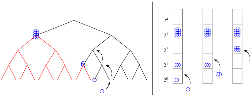
Figure 1: A residue going up the radix ladder

Then to recover the whole reconstructed number it is sufficient to iterate through the ladder from the ground level and make all the encountered partial results go to up one level after the other to the top of the ladder. As we will see in section 3.3, LinBox-1.1.7 contains such a data structure, in linbox/algorithms/cra-full-multip.h.

An advantage of this structure is that it enables insertion of any size pair with fast arithmetic complexity. Moreover, merge of two ladders is straightforward and we will make an extensive use of that fact in a parallel setting in section 5.

Algorithm 3 RadixLadder.merge

0:  Two radix ladders $RL_{1}$ and $RL_{2}$.

0:  In place merge of $RL_{1}$ and $RL_{2}$.

1:  for $i=0$ to size$(RL_{2})$ do

2:     $RL_{1}$.insert($RL_{2}$.Shelf$[i]$);

3:  end for

4:  Return $RL_{1}$

3 A Chinese remaindering design pattern

The generic design we propose here comes from the observation that there are in general two ways of computing a reconstruction: a deterministic way computing all the residues until the product of moduli reaches a bound on the size of the result ; or a probabilistic way using early termination. We thus propose an abstraction of the reconstruction process in three layers: a black box function produces residues modulo small moduli, an integer builder produces reconstructions using algorithm 2, and a Chinese remaindering controller commands them both.

Here our point is that the controller is completely generic where the builder may use e.g. the radix ladder data structure proposed in section 2 and has to implement the termination strategy.

3.1 Black box residue computation

In general this consists in mapping the problem from $\mathbb{Z}$ to $\leavevmode\kern 1.00006pt\raise 0.0pt\hbox{$\mathbb{Z}$}\kern-1.00006pt/\kern-1.49994pt\lower 1.29167pt\hbox{$m$}\mbox{$\mathbb{Z}$}$ and computing the result modulo $m$. Such black boxes are defined e.g. for the determinant, valence, minpoly, charpoly, linear system solve as function objects IntegerModular* (where * is one of the latter functions) in the linbox/solutions directory of LinBox-1.1.7.

3.2 Chinese remaindering controller

The pattern we propose here is generic with respect to the termination strategy and the integer reconstruction scheme. The controller must be able to initialize the data structure via the builder ; generate some coprime moduli ; apply the black box function ; update the data structure ; test for termination and output the reconstructed element. The generations of moduli and the black box are parameters and the other functionalities are provided by any builder. Then the control is a simple loop. Algorithm 4 shows this loop which contains also the whole interface of the Builder.

Algorithm 4 CRA-Control

1:  $Builder$.initialize$()$;

2:  while $Builder$.notTerminated$()$ do

3:     $p:=Builder.$nextCoPrime$()$;

4:     $v:=BlackBox$.apply$(p)$;

5:     $Builder$.update$(v,p)$;

6:  end while

7:  Return $Builder$.reconstruct$()$;

LinBox-1.1.7 gives an implementation of such a controller, parametrized by a builder and a black box function as the class ChineseRemainder in linbox/algorithms/cra-domain.h.

The interface of a controller is to be a function class. It contains a constructor with a builder as argument and the functional operator taking as argument a BlackBox, computing e.g. a determinant modulo $m$, and a moduli generator and returning an integer reconstructed from the modular computations. Algorithm 5 shows the specifications of the LinBox-1.1.7 controller.

Algorithm 5 C++ ChineseRemainder class

⬇

1template<class Builder> struct ChineseRemainder {

2ChineseRemainder(const Builder& b) : builder_(b) {}

3template<class Function> Integer& operator() (

4 Integer & res,

5 const Function & BlackBox) {

6 // CRA-Control …

7}

8const Builder& getBuilder() { return builder_; }

9protected: Builder builder_;

10};

Then any higher-level algorithm just choose its builder and its controller and pass them the modular BlackBox iteration it wants to lift over the integers.

3.3 Integer builders

The role of the builder is to implement the interface defined by algorithm 4.

There are already three of these implementations in LinBox-1.1.7: an early terminated for a single residue, an early terminated for a vector of residues and a deterministic for a vector of residues (resp. the files cra-early-single.h, cra-early- multip.h and cra-full-multip.h in the linbox/algorithms directory). Up to now the radix ladder is not a separated class as only this data structure is currently used and as it is simple enough to inherit from one of the latter and modify the behavior of the methods.

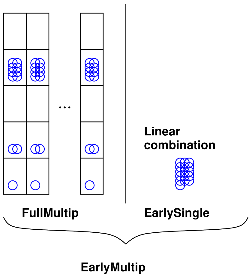
Figure 2: Early termination of a vector of residues via a linear combination

Actually EarlyMultipCRA inherits from both EarlySingleCRA and FullMultipCRA as it uses the radix ladder of FullMultipCRA for its reconstruction and the early termination of EarlySingleCRA to test a linear combination of the residues to be reconstructed as shown on figure 2 The FullMultipCRA has been implemented so that when a vector/matrix is reconstructed the moduli and some computations are shared among the ladders. We give more implementation details on the early termination strategies in sections 4 and 5.

3.4 Mappers and binders

To further enhance genericy, the mapping of between integer and field operations can also be automatized. If the data structure storing the matrix disposes of binder adaptors generic mappers can be designed. This is the case for the sparse and dense matrices of linbox and a generic converter, using the Givaro/LinBox fields init and convert converters, can be found in linbox/field/hom.h, linbox/algorithm/matrix-hom.h.

Then, to map any function class to the field representation one can use the following generic mapper:

Algorithm 6 C++ Mapper class

⬇

1template<class Data, class Function>

2struct Mapper {

3 Mapper(const Data &b, const Function& h)

4 : A(b), g(h) {}

5

6 template<class Field> typename Field::Element&

7 operator() (typename Field::Element& d,

8 const Field& F) const {

9 typename Data::template rebind<Field>::other Ap;

10 Homomorphism::map(Ap, this->A, F);

11 return this->g( d, Ap );

12 }

13

14protected: const Data& A; const Function& g;

15};

An example of the design usage, here computing a determinant via Chinese remaindering, is then simply:

Algorithm 7 C++ Chinese remaindering scheme

⬇

1// […] builder, matrix initializations etc.

2ChineseRemainder<ModularEarlySingleCRA> ETcra(Builder);

3Mapper<SparseMatrix<Integer>,Determinant> BBox(A,Det);

4Integer d;

5

6ETcra( d, BBox); // Call to the controller

4 Termination strategies

We sketch here several termination strategies and show that our design enables to modify this strategy and only that while the rest of the implementation is unchanged.

4.1 Deterministic strategy

There $Full*CRA$.update$(v,p)$ just adds the residues to the ladder ; where $Full*CRA$.notTerminated$()$ tests if the product of primes so far exceeds the precomputed deterministic bound.

4.2 Earliest termination

In a sequential mode, depending on the actual speed of the different routines of table 1 on a specific architecture or if the cost of $BlackBox$.apply is largely dominant, one can choose to test for termination after each call to the black box. A way to implement the probabilistic test of [12, Lemma 3.1] and to reuse every black box apply is to use random primes as the moduli generator. Indeed then the probabilistic check can be made with the incoming black box residue computed modulo a random prime. The reconstruction algorithm of section 3 is then only slightly modified as shown in algorithm 8

Algorithm 8 EarlySingleCRA.update$(v,p)$

0:  $U\equiv R\mod M$.

0:  A variable $Stabilization$ initially set to $0$.

0:  $v\equiv R\mod p$.

0:  $R_{MN}\equiv R\mod M\times p$.

1:  $u\equiv U\mod p$;

2:  if $u==v$ then

3:     Increment $Stabilization$;

4:     Return $(U,M\times p)$;

5:  else

6:     $Stabilization=0$;

7:     Return Reconstruct$(U\mod M,v\mod p)$;

8:  end if

and the termination test becomes simply algorithm 9.

Algorithm 9 EarlySingleCRA.notTerminated$()$

1:  Return $Stabilization<EarlyTerminationThreshold$;

In the latter algorithm, $EarlyTerminationThreshold$ is the number of successive stabilizations required to get a probabilistic estimate of failures. It will be denoted $ET$ for the rest of the paper. This is the strategy implemented in LinBox-1.1.7 in linbox/algorithms/cra-early-single.h. With the estimates of table 1, the cost of the whole reconstruction of algorithm 4 thus becomes

$$\small\sum_{i=1}^{t}\left(\text{\bf apply}+8i+O(1)\right)=\\ (t+ET)\text{\bf apply}+4(t+ET)^{2}+O(t)$$ (2)

where $t=\lceil\log_{2^{\beta}}(R)\rceil$ and $\beta$ is the word size.

This strategy enables the least possible number of calls to $BlackBox$.apply. It it thus useful when the latter dominates the cost of the reconstruction.

4.3 Balanced termination

Another classic case is when one wants to use fast integer arithmetic for the reconstruction. Then the balanced computations are mandatory and the radix ladder becomes handy. The problem now becomes the early termination. There a simple strategy could be to test for termination only when the number of computed residues is a power of two. In that case the reconstruction is guaranteed to be balanced and fast Chinese remaindering is also guaranteed. Moreover random moduli are not any more necessary for all the residues, only those testing for early termination need be randomly generated. This induces another saving if one fixes the other primes and precomputes all the factors $M_{i}\times(M_{i}^{-1}\mod M_{i+1})$. There the cost of the reconstruction drops by a factor of $2$ from $2(m_{\alpha}+d_{\alpha})l^{\alpha}$ to $(m_{\alpha}+d_{\alpha})l^{\alpha}$.
The drawback is an extension of the number of black box applications from $\lceil\log_{2^{\beta}}(R)\rceil+ET$ to the largest power of two immediately superior and thus up to a factor of $2$ in the number of black box applies. For the $Builder$, the update becomes just a push in the ladder as shown on algorithm 10.

Algorithm 10 EarlyBalancedCRA.update$(v,p)$

1:  RadixLadder.insert$(v,p)$;

The termination condition, on the contrary tests only when the number of residues is power of two as shown on algorithm 11.

Algorithm 11 EarlyBalancedCRA.notTerminated$()$

1:  if Only one Shelf, Shelf$[i]$, is full then

2:     Set $U_{i}$ to Shelf$[i]$ residue;

3:     for $j=1$ to  $EarlyTerminationThreshold$ do

4:        $p:=$PrimeGenerator$()$;

5:        if $(U_{i}\mod p)~{}~{}!=~{}BlackBox$.apply$(p)$ then

6:           Return $false$;

7:        end if

8:     end for

9:     Return $true$;

10:  else

11:     Return $false$;

12:  end if

Then, the whole reconstruction of algorithm 4 now requires:

$$\begin{split}ET\cdot(\text{\bf apply}+3\cdot 2^{k})+\sum_{i=0}^{k-1}\frac{2^{k}}{2^{i+1}}\left(\text{\bf apply}+(m_{\alpha}+d_{\alpha})2^{i\alpha}\right)\\ +(\text{\bf apply}+3\cdot 2^{i})=\\ (2^{k}+k+ET-1)\cdot\text{\bf apply}+\left(2^{k}\right)^{\alpha}\frac{m_{\alpha}+d_{\alpha}}{2^{\alpha}-2}+O(2^{k})\end{split}$$ (3)

operations, where now $k=\lceil\log_{2}(\log_{2^{\beta}}(R))\rceil$.

Despite the augmentation in the number of black box applications, the latter can be useful, in particular when multiple values are to be reconstructed.

Example 1.

Consider the Gaußian elimination of an integer matrix where all the matrix entries are larger than $n$ and bounded in absolute value by $A_{\infty}$. Let $a_{\infty}=\log_{2^{\beta}}(A_{\infty})$ and suppose one would like to compute the rational coefficients of the triangular decomposition only by Chinese remaindering (there exist better output dependant algorithms, see e.g. [22], but usually with the same worst-case complexity). Now, Hadamard bound gives that the resulting numerators and denominators of the coefficients are bounded by $\sqrt{nA_{\infty}^{2}}^{n}$. Then the complexity of the earliest strategy would be dominated by the reconstruction where the balanced strategy or the hybrid strategy of figure 2 could benefit from fast algorithms:

EarlySingleCRA	$O(n^{4}a_{\infty}^{2})$
EarlyMultipCRA	$O(n^{\omega+1}a_{\infty}+n^{2+\alpha}a_{\infty}^{\alpha}+n^{2}a_{\infty}^{2})$
EarlyBalancedCRA	$O(2n^{\omega+1}a_{\infty}+n^{2+\alpha}a_{\infty}^{\alpha})$

Table 2: Early termination strategies complexities for Chinese remaindered Gaußian elimination with rationals

In the case of small matrices with large entries the reconstruction dominates and then a balanced strategy is preferable. Now if both complexities are comparable it might be useful to reduce the factor of $2$ overhead in the black box applications. This can be done via amortized techniques, as shown next.

4.4 Amortized termination

A possibility is to use the $\rho$-amortized control of [2]: instead of testing for termination at steps $2^{1}$, $2^{2}$, $\ldots$, $2^{i}$, $\ldots$ the tests are performed at steps $\rho^{g(1)}$, $\rho^{g(2)}$, $\ldots$, $\rho^{g(i)}$, $\ldots$ with $1<\rho<2$ and $g$ satisfies $\forall i$, $g(i)\leq i$. If the complexity of the modular problem is $C$ and the number of iterations to get the output is $b$, [2] give choices for $\rho$ and $g$ which enable to get the result with only $b+\frac{f(b)}{b}$ iterations and extra $O(f(b))$ termination tests where $f(b)=log_{\rho}(b)$.

In example 1 the complexity of the modular problem is $n^{\omega}$, the size of the output and the number of iterations is $na_{\infty}$ so that strategy would reduce the iteration complexity from $2n^{\omega+1}a_{\infty}$ to $(na_{\infty}+o(na_{\infty}))n^{\omega}$ and the overall complexity would then become:

EarlyAmortizedCRA	$O(n^{\omega+1}a_{\infty}+n^{2+\alpha}a_{\infty}^{\alpha}$
	$+\log(na_{\infty})n^{\alpha}a_{\infty}^{\alpha})$

Indeed, we suppose that the amortized technique is used only on a linear combination, and that the whole matrix is reconstructed with a FullMultipCRA, as in figure 2. Then the linear combination has size $2\log(n)+n\cdot a_{\infty}$ which is still $O(n\cdot a_{\infty})$. Nonetheless, there is an overhead of a factor $\log(na_{\infty})$ in the linear combination reconstruction since there might be up to $O(\log(na_{\infty}))$ values $\rho^{g(i)}$, $\rho^{g(i+1)}$, $\ldots$ between any two powers of two. Overall this gives the above estimate. Now one could use other $g$ functions as long as eq. 4 is satisfied.

$$\begin{cases}\left(\rho^{g(i+1)}-\rho^{g(i)}\right)=o(\rho^{g(i)})\\ \left(\rho^{g(i+k(i))}-\rho^{g(i)}\right)\sim 2^{\lceil\log_{2}(\rho^{g(i)})\rceil},&k(i)=o(\rho^{g(i)})\end{cases}$$ (4)

5 Parallelization

All parallel versions of these sequential algorithms have to consider the parallel merge of radix ladders and the parallelization of the loop of the CRA-control algorithm 4. Many parallel libraries can be used, namely OpenMP or Cilk would be good candidates for the parallelization of the embarrassingly parallel FullMultipCRA. Now in the early termination setting, the main difficulty comes from the distribution of the termination test. Indeed, the latter depends on data computed during the iterations. To handle this issue we propose an adaptive parallel algorithm [5, 24] and use the Kaapi library [6, 16]. Its expressiveness in an adaptive setting guided our choice, together with the possibility to work on heterogenous networks.

5.1 Kaapi overview

Kaapi is a task based model for parallel computing. It was targeted for distributed and shared memory computers. The scheduling algorithm uses work-stealing [3, 1, 4, 17]: an idle processor tries to steal work to a randomly selected victim processor.

The sequential execution of a Kaapi program consists in pushing and popping tasks to dequeue the current running processor. Tasks should declare the way they access the memory, in order to compute, at runtime, the data flow dependencies and the ready tasks (when all their input values are produced). During a parallel execution, a ready task, in the queue but not executed, may be entirely theft and executed on an other processor (possibly after being communicated through the network). These tasks are called dfg tasks and their schedule by work-stealing is described in [16, 17].

A task being executed by a processor may be only partially theft if it interacts with the scheduler, in order to e.g. decide which part of the work is to be given to the thieves. Such tasks are called adaptive tasks and allows fine grain loop parallelism.

To program an adaptive algorithm with Kaapi, the programmer has to specify some points in the code (using kaapi_stealpoint) or sections of the code (kaapi_stealbegin, kaapi_stealend) where thieves may steal work. To guarantee that parallel computation is completed, the programmer has to wait for the finalization of the parallel execution (using kaapi_steal_finalize). Moreover, in order to better balance the work load, the programmer may also decide to preempt the thieves (send an event via kaapi_preempt_next).

5.2 Parallel earliest termination

Algorithm 12 lets thieves steal any sequence of primes.

Algorithm 12 ParallelCRA-Control

1:  $Builder$.initialize$()$;

2:  while $Builder$.notTerminated$()$ do

3:     $p:=Builder.$nextCoPrime$()$;

4:      kaapi_stealbegin$(\ splitter,\ Builder)$;

5:     $v:=BlackBox$.apply$(p)$;

6:     $Builder$.update$(v,p)$;

7:     kaapi_finalize_steal$()$;

8:      kaapi_stealend();

9:     if require synchronization step then

10:        while kaapi_nomore_thief$()$ do

11:           $(list\ of\ v,list\ of\ p):=$kaapi_preempt_next();

12:            $Builder$.update$(list\ of\ v,list\ of\ p)$;

13:        end while

14:     end if

15:  end while

16:  Return $Builder$.reconstruct$()$;

At line 4, the code allows the scheduler to trigger the processing of steal requests by calling the $splitter$ function. The parameters of kaapi_stealbegin are the $splitter$ function and some arguments to be given to its call. These arguments can e.g. specify the state of the computation to modify (here the builder object plays this role). Then, on the one hand, concurrent modifications of the state of computation by thieves, must be taken care of during the control flow between lines 4 and 8: here the computation of the residue could be evaluated by multiple threads without critical section. On the other hand, after line 8, the scheduler guarantees that no concurrent thief can modify the computational state when they steal some work. Remark that both branches of the conditional if at line 9 must be executed without concurrency: the iteration of the list of thieves or the generation of the next random modulus are not reentrant.

The role of the $splitter$ function is to distribute the work among the thieves. In algorithm 13, each thief receives a coPrimeGenerator object and the $entrypoint$ to execute.

Algorithm 13 Splitter$(Builder,N,requests[])$

1:  for $i=0$ to $N-1$ do

2:     kaapi_request_reply$(request[i],entrypoint,$ $\hskip 28.45274ptBuilder.getCoPrimeGenerator()\ )$;

3:  end for

The coPrimeGenerator depends on the Builder type and allows the thief to generate a sequence of moduli. For instance the coPrimeGenerator for the earliest termination contains at one point a single modulus $M$ which is returned by the next call of nextCoPrime() by the Builder.

The $splitter$ function knows the number $N$ of thieves that are trying to steal work to the same victim. Therefore it allows for a better balance of the work load. This feature is unique to Kaapi when compared to other tools having a work-stealing scheduler.

5.3 Synchronization

Now, the victim periodically tests the global termination of the computation (line 9 of algorithm 12). Depending on the chosen termination method (Early*CRA, etc.), the synchronization may occur at every iteration or after a certain number of iterations. The choice is made in order to e.g. amortize the cost of this synchronization or reduce the arithmetic cost of the reconstruction. Then each thief is preempted (line 11) and the code recovers its results before giving them to the Builder for future reconstruction (line 12).

The preemption operation is a two way communication between a victim and a thief: the victim may pass parameters and get data from one thief. Note that the preemption operation assumes cooperation with the thief code. The latter being responsible for polling incoming events at specific points (e.g. where the computational state is safe preemption-wise).

On the one hand, to amortize the cost of this synchronization, more primes should be given to the thieves. In the same way, the victim code works on a list of moduli inside the critical section (at line 3 returns a list of moduli, and at lines 5-6 the victim iterates over this list by repeatedly calling apply and update methods). On the other hand, to avoid long waits of the victim during preemption, each thief should test if it has been preempted to return quickly its results (see next section).

5.4 Thief entrypoint

Finally, algorithm 14 returns both the sequence of residues and the sequence of primes that where given to the BlackBox. This algorithm is very similar to algorithm 12.

Algorithm 14 Thief’s EntryPoint(M)

1:  $Builder$.initialize$()$;

2:  $list\ of\ v$.clear$()$;

3:  $list\ of\ p$.clear$()$;

4:  while $Builder$.CoPrimeGenerator$()$ not empty do

5:     if kaapi_preemptpoint$()$ then break; end if 

6:     $p:=Builder.$nextCoPrime$()$;

7:      kaapi_stealbegin$(\ splitter,\ Builder)$;

8:     $list\ of\ p$.push_back$(p)$;

9:     $list\ of\ v$.push_back$(BlackBox$.apply$(p))$;

10:      kaapi_stealend();

11:  end while

12:  kaapi_stealreturn $(list\ of\ v,list\ of\ p)$;

Lines 7 and 10 define a section of code that could be concurrent with steal requests. At line 5, the code tests if a preemption request has been posted by algorithm 12 at line 11. If this is the case, then the thief aborts any further computation and the result is only a partial set of the initial work allocated by the $splitter$ function.

5.5 Efficiency

These parallel versions of the Chinese remaindering have been implemented using Kaapi transparently from the LinBox library: one has just to change the sequential controller cra-domain.h to the parallel one.

In LinBox-1.1.7 some of the sequential algorithms which make use of some Chinese remaindering are the determinant, the minimal/characteristic polynomial and the valence, see e.g. [20, 12, 11, 8] for more details.

We have performed these preliminary experiments on an 8 dual core machine (Opteron 875, 1MB L2 cache, 2.2Ghz, with 30GBytes of main memory). Each processor is attached to a memory bank and communicates to its neighbors via an hypertransport network. We used g++ 4.3.4 as C++ compiler and the Linux kernel was the 2.6.32 Debian distribution.

All timings are in seconds. In the following, we denote by $T_{seq}$ the time of the sequential execution and by $T_{p}$ the time of the parallel execution for $p=8$ or $p=16$ cores. All the matrices are from “Sparse Integer Matrix Collection” (SIMC).

Table 3 gives the performance of the parallel computation of the determinant for small invertible matrices (less than a second) and larger ones (an hour CPU) of the SIMC/SPG and SIMC/Trefethen collections.

$$\begin{array}[]{|c|c||c|c|c|}\hline\cr\bf Matrix&\bf d,r&\bf T_{seq}[k]&\bf T_{p=8}[k]&\bf T_{p=16}[k]\\ \hline\cr\hline\cr ex-1&560,\ 8736&0.29[4]&0.16[9]&0.22[16.8]\\ ex-3&2600,\ 71760&837.80[184]&123.56[193]&77.99[193]\\ \hline\cr t-150&150,\ 2040&0.21[59]&0.046[63.4]&0.036[63.6]\\ t-300&300,\ 4678&2.52[138]&0.36[144.8]&0.24[144.7]\\ t-500&500,\ 8478&15.19[249]&2.05[257]&1.31[256.3]\\ t-700&700,\ 12654&52.59[367]&6.50[368.9]&4.19[371.2]\\ t-2000&2000,\ 41907&2978.23[1274]&384.43[1281]&236.59[1281]\\ \hline\cr\end{array}$$

Table 3: Timings for the computation of the determinant. $d$ is the dimension of the matrix, $r$ the number of non-zero coefficients, $[k]$ is the mean number of primes observed for the Chinese remaindering using $p$ cores.

The small instance (ex-1) needed very few primes to reconstruct integer the solution. There, we can see the overhead of parallelism: this is due to some extra synchronizations and also to the large number of unnecessary modular computations before realizing that early termination was needed. Despite this we do achieve some speed-up.

We show on table 4 the corresponding speed-ups of table 3 compared with a naive approach using OpenMP: for $p$ the number available cores, launch the computations by blocks of $p$ iterations and test for terminaison after each block is completed.

$$\begin{array}[]{|c||c|c||c|c|c|c|c|}\hline\cr Matrix&ex-1&ex-3&t-150&t-300&t-500&t-700&t-2000\\ \hline\cr Naive&\bf 1.38&10.66&2.10&8.52&11.29&12.55&12.48\\ Alg.\ref{alg:parcontrol}&1.35&\bf 10.74&\bf 5.78&\bf 10.52&\bf 11.56&12.55&\bf 12.59\\ \hline\cr\end{array}$$

Table 4: Speed-up using $16$ cores of algorithm 12 compared to a naive approach with OpenMP

For large computations the speed-up is quite the same since the computation is largely dominant. For smaller instances we see the advantage of reducing the number of synchronizations. On e.g. multi-user environments the advantage should be even greater.

6 Conclusion

We have proposed a new data structure, the radix ladder, capable of managing several kinds of Chinese reconstructions while still enabling fast reconstruction.

Then, we have defined a new generic design for Chinese remaindering schemes. It is summarized on figure 3. Its main feature is the definition of a builder interface in charge of the reconstruction. This interface is such that any of termination (deterministic, early terminated, distributed, etc.) can be handled by a CRA controller. It enables to define and test remaindering strategies while being transparent to the higher level routines. Indeed we show that the Chinese remaindering can just be a plug-in in any integer computation.

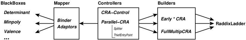
Figure 3: Generic Chinese remaindering scheme

We also provide in LinBox-1.1.7 an implementation of the ladder, several implementations for different builders and a sequential controller. Then we tested the introduction of a parallel controller, written with Kaapi, without any modification of the LinBox library. The latter handles the difficult issue of distributed early termination and shows good performance on a SMP machine.

In parallel, some improvement could be made to the early termination strategy in particular when the BlackBox is fast compared to the reconstruction and when balanced and amortized techniques are required. Also, output sensitive early termination is very useful for rational reconstruction, see e.g. [21] and thus the latter should benefit from this kind of design.

References

- [1] N. S. Arora, R. D. Blumofe, and C. G. Plaxton. Thread scheduling for multiprogrammed multiprocessors. In Proceedings of the Tenth Annual ACM Symposium on Parallel Algorithms and Architectures (SPAA’01), Puerto Vallarta, pages 119–129, 2001.
- [2] O. Beaumont, E. M. Daoudi, N. Maillard, P. Manneback, and J.-L. Roch. Tradeoff to minimize extra-computations and stopping criterion tests for parallel iterative schemes. In 3rd International Workshop on Parallel Matrix Algorithms and Applications (PMAA04), CIRM, Marseille, France, Oct. 2004.
- [3] R. Blumofe, C. Joerg, B. Kuszmaul, C. Leiserson, K. Randall, and Y. Zhou. Cilk: An efficient multithreaded runtime system. Journal of Parallel and Distributed Computing, 37(1):55–69, 1996.
- [4] D. Chase and Y. Lev. Dynamic circular work-stealing deque. In P. B. Gibbons and P. G. Spirakis, editors, Proceedings of the 17th Annual ACM Symposium on Parallel Algorithms (SPAA’05), Las Vegas, Nevada, USA, pages 21–28. ACM, July 2005.
- [5] V. D. C. Cung, V. Danjean, J.-G. Dumas, T. Gautier, G. Huard, B. Raffin, C. Rapine, J.-L. Roch, and D. Trystram. Adaptive and hybrid algorithms: classification and illustration on triangular system solving. In Dumas [7], pages 131–148.
- [6] V. Danjean, R. Gillard, S. Guelton, J.-L. Roch, and T. Roche. Adaptive loops with kaapi on multicore and grid: Applications in symmetric cryptography. In Watt [25], pages 33–42.
- [7] J.-G. Dumas, editor. TC’2006. Proceedings of Transgressive Computing 2006, Granada, España. Universidad de Granada, Spain, Apr. 2006.
- [8] J.-G. Dumas. Bounds on the coefficients of the characteristic and minimal polynomials. Journal of Inequalities in Pure and Applied Mathematics, 8(2):art. 31, 6 pp, Apr. 2007.
- [9] J.-G. Dumas, T. Gautier, M. Giesbrecht, P. Giorgi, B. Hovinen, E. Kaltofen, B. D. Saunders, W. J. Turner, and G. Villard. LinBox: A generic library for exact linear algebra. In A. M. Cohen, X.-S. Gao, and N. Takayama, editors, Proceedings of the 2002 International Congress of Mathematical Software, Beijing, China, pages 40–50. World Scientific Pub., Aug. 2002.
- [10] J.-G. Dumas, P. Giorgi, and C. Pernet. Dense linear algebra over prime fields. ACM Transactions on Mathematical Software, 35(3):1–42, Nov. 2008.
- [11] J.-G. Dumas, C. Pernet, and Z. Wan. Efficient computation of the characteristic polynomial. In M. Kauers, editor, Proceedings of the 2005 ACM International Symposium on Symbolic and Algebraic Computation, Beijing, China, pages 140–147. ACM Press, New York, July 2005.
- [12] J.-G. Dumas, B. D. Saunders, and G. Villard. On efficient sparse integer matrix Smith normal form computations. Journal of Symbolic Computation, 32(1/2):71–99, July–Aug. 2001.
- [13] J.-G. Dumas and A. Urbańska. An introspective algorithm for the determinant. In Dumas [7], pages 185–202.
- [14] I. Z. Emiris. A complete implementation for computing general dimensional convex hulls. International Journal of Computational Geometry and Applications, 8(2):223–253, Apr. 1998.
- [15] J. v. Gathen and J. Gerhard. Modern Computer Algebra. Cambridge University Press, New York, NY, USA, 1999.
- [16] T. Gautier, X. Besseron, and L. Pigeon. KAAPI: A thread scheduling runtime system for data flow computations on cluster of multi-processors. In Watt [25], pages 15–23.
- [17] T. Gautier, J. L. Roch, and F. Wagner. Fine grain distributed implementation of a dataflow language with provable performances. In Workshop PAPP 2007 - Practical Aspects of High-Level Parallel Programming in International Conference on Computational Science 2007 (ICCS2007), Beijing, China, may 2007. IEEE.
- [18] A. Goldstein and R. Graham. A Hadamard-type bound on the coefficients of a determinant of polynomials. SIAM Review, 15:657–658, 1973.
- [19] T. Granlund and P. L. Montgomery. Division by invariant integers using multiplication. In Proceedings of the ACM SIGPLAN ’94 Conference on Programming Language Design and Implementation, pages 61–72, Orlando, Florida, June 20–24, 1994.
- [20] E. Kaltofen. An output-sensitive variant of the baby steps/giant steps determinant algorithm. In T. Mora, editor, Proceedings of the 2002 ACM International Symposium on Symbolic and Algebraic Computation, Lille, France, pages 138–144. ACM Press, New York, July 2002.
- [21] S. Khodadad and M. Monagan. Fast rational function reconstruction. In J.-G. Dumas, editor, Proceedings of the 2006 ACM International Symposium on Symbolic and Algebraic Computation, Genova, Italy, pages 184–190. ACM Press, New York, July 2006.
- [22] C. Pernet and W. Stein. Fast computation of hermite normal form of random integer matrices. Technical report, 2009. http://modular.math.washington.edu/papers/hnf/hnf.pdf.
- [23] C. Pernet and A. Storjohann. Faster algorithms for the characteristic polynomial. In C. W. Brown, editor, Proceedings of the 2007 ACM International Symposium on Symbolic and Algebraic Computation, Waterloo, Canada. ACM Press, New York, July 29 – August 1 2007.
- [24] D. Traore, J.-L. Roch, N. Maillard, T. Gautier, and J. Bernard. Adaptive parallel algorithms and applications to STL. In Springer-Verlag, editor, EUROPAR 2008, Las Palmas, Spain, August 2008.
- [25] S. Watt, editor. Parallel Symbolic Computation’07. Waterloo University, Ontario, Canada, July 2007.