Definitions of entanglement entropy of spin systems in the valence-bond basis

Abstract

The valence-bond structure of spin-1/2 Heisenberg antiferromagnets is closely related to quantum entanglement. We investigate measures of entanglement entropy based on transition graphs, which characterize state overlaps in the overcomplete valence-bond basis. The transition graphs can be generated using projector Monte Carlo simulations of ground states of specific hamiltonians or using importance-sampling of valence-bond configurations of amplitude-product states. We consider definitions of entanglement entropy based on the bonds or loops shared by two subsystems (bipartite entanglement). Results for the bond-based definition agrees with a previously studied definition using valence-bond wave functions (instead of the transition graphs, which involve two states). For the one dimensional Heisenberg chain, with uniform or random coupling constants, the prefactor of the logarithmic divergence with the size of the smaller subsystem agrees with exact results. For the ground state of the two-dimensional Heisenberg model (and also Néel-ordered amplitude-product states), there is a similar multiplicative violation of the area law. In contrast, the loop-based entropy obeys the area law in two dimensions, while still violating it in one dimension—both behaviors in accord with expectations for proper measures of entanglement entropy.

I Introduction

The concept of quantum mechanical entanglement is of broad interest in physics. One widely used quantitative measure of entanglement is the von Neumann entanglement entropy $S_{\rm vN}$. Partitioning a many-body system in a pure quantum state into two contiguous subsystems, $S_{\rm vN}$ is defined as the von Neumann entropy of the reduced density matrix of either one of the two subsystems. The insight that $S_{\rm vN}$ typically scales proportionally to the boundary area (the area law EISERT ) was first developed in the context of black holes.SREDN The area law has now become a key benchmark for characterizing states of interest in quantum information theory KITAEV ; WOLF and condensed matter physics.LEVIN ; FRADKIN An important application of this concept is to construct computationally tractable variational ansätze for ground states based on the area law.TENSOR ; TAGLIA

While $S_{\rm vN}$ is a clear and well established measure of entanglement, it is difficult to compute for strongly-correlated quantum systems in dimensions higher than one, where exact diagonalization and density matrix renormalization group approaches become inefficient.DMRG ; LADDER Alternative definitions of entanglement entropy (or, more precisely, alternative measures of entanglement) are therefore also actively investigated. The Rényi entropies $S_{n}$ ($n=1,2,\ldots$) are often used,LI and have the appealing property that $S_{1}=S_{\rm vN}$. Recently it was realized RENYI that $S_{2}$ (and in principle also $S_{n}$ for $n>2$) can be computed for quantum spin systems using projector quantum Monte Carlo (QMC) simulations in the valence bond (VB) basis.SANDVIK Previously, a measure $S_{\text{VB}}$ of entanglement entropy explicitly making use of the VB basis was also introduced VBE1 ; VBE2 within the context of this QMC method. Generalizing an exact result for a single VB state REFAEL to a superposition, $S_{\text{VB}}$ is given by the average number of VBs connecting two subsystems. While defined explicitly using the VB basis, this quantity also can be evaluated using the density matrix renormalization group (DMRG) method CAPPONI and is, therefore, not completely tied to the VB basis. Its asymptotic behavior has also been found exactly using analytical methods for the Heisenberg chain.JACOBSEN

In this paper, we formulate a different measure $S_{\rm VB}^{2}$ of entanglement entropy for quantum spin systems in terms of the transition graphs characterizing overlaps of VB basis states. The transition graphs are generated in projector Monte Carlo simulations of the ground state of a hamiltonian,SANDVIK ; LOOP or in Monte Carlo sampling of bond configurations of variational states such as the amplitude product states.LIANG1 ; LOOP Like the previous definition of VB entanglement entropy, which we henceforth call $S_{\text{VB}}^{1}$, the transition-graph definition $S_{\rm VB}^{2}$ involves VBs shared by two subsystems, but the weighting is different because the bond configurations in the projected bra and ket states are sampled using their individual wave functions and overlap (which depends on the number of loops in the transition graph). We show that $S_{\rm VB}^{2}$ scales with the subsystem size in accord with an exact result JACOBSEN for the previous definition $S_{\rm VB}^{1}$ in the one dimensional (1D) Heisenberg chain. The corrections to this form are much smaller than in the previous definition, however. Thus, the different weighting procedure appears to reduce the subleading size corrections.

Both $S_{\rm VB}^{1}$ and $S_{\rm VB}^{2}$ violate the area law in the case of the Néel-ordered ground state of the two-dimensional (2D) Heisenberg model. We here argue that this is because definitions based on single VBs typically will overestimate the entanglement, due to the over-completeness of the VB basis. To remedy this, we propose an alternative measure $S_{\rm loop}$ of entanglement entropy based on the loops of the transition graphs, i.e., $S_{\rm loop}$ is the average number of transition-graph loops shared by the two subsystems. Loops correspond to maximally entangled groups of spins, and the number of loops shared by the subsystems is therefore an appropriate measure of entanglement. We show that $S_{\rm loop}$ of the 2D Heisenberg model (and also in a generic variational amplitude-product state with Néel order) obeys the area law and has an additive logarithmic correction, in contrast to the multiplicative logarithmic corrections affecting the bond-based definitions. Thus, it appears that the loop entropy scales in the same way as the Rényi entropy (as observed in Ref. RENYI, ) and the standard von Neumann entanglement entropy (where one would expect such scaling) and, thus, may be a convenient (more easily computable) stand-in for these definitions.

The outline of the rest of the paper is as follows. In Sec. II we summarize the properties of the VB basis needed for our definitions and calculations, and also briefly review amplitude-product states,LIANG1 the VB projector QMC method,SANDVIK ; LOOP and the loop-gas picture SUTHER1 ; SUTHER2 of VB states. The VB and loop entropy definitions are discussed and tested in Secs. III and IV. We conclude in Sec. V with a summary and discussion.

II Valence-bond basis and methods

We will consider the spin-$1/2$ Heisenberg hamiltonian, written in the form

$$H=-\sum_{\langle{i,j}\rangle}J_{ij}S_{ij},~{}~{}~{}~{}~{}(J_{ij}>0),$$ (1)

where $\langle{i,j}\rangle$ denotes nearest-neighbor spins on a lattice with periodic boundaries and $S_{ij}$ is a singlet projector,

$$S_{ij}=1/4-\mathbf{S}_{i}\cdot\mathbf{S}_{j},$$ (2)

and $J_{ij}>0$ are antiferromagnetic coupling constants. We will study 1D chains with uniform and random couplings, as well as uniform 2D square lattices.

Here, in Sec. II.1, we discuss the VB basis in which we carry out all calculations. In Sec. II.2 we discuss variational VB amplitude-product states, which give some important insights into various types of ground states and their entanglement properties. The projector QMC calculations that we use for unbiased calculations are briefly reviewed in Sec. II.3. The loop-gas picture of VB states was first introduced by Sutherland.SUTHER1 ; SUTHER2 In Sec. II.4 we discuss it in a somewhat broader sense, which we will rely on for the definition of loop entropy in Sec. IV.

II.1 The valence-bond basis

The ground state of $H$ on a bipartite lattice with an even number $N$ of spins is a total-spin singlet and can be expanded in bipartite VB states (i.e., each bond connects sites on the two sublattices) with all positive coefficients;LIANG1

$$\left|{\psi_{0}}\right\rangle=\sum_{v}\lambda_{v}\left|{v}\right\rangle,~{}~{}~{}~{}(\lambda_{v}\geq 0\;\forall~{}v).$$ (3)

With the singlet state of two spins $i,j$ denoted by $(i,j)$, a bipartite VB basis state is defined as

$$\left|{v}\right\rangle:=\bigotimes_{ij}(i,j),~{}~{}~{}~{}(i,j):=\frac{1}{\sqrt{2}}\bigl{(}\left|{\uparrow_{i}\downarrow_{j}}\right\rangle-\left|{\downarrow_{i}\uparrow_{j}}\right\rangle\bigr{)},$$ (4)

where sites $i$ and $j$ are on different sublattices and each site appears exactly once in the product. Thus, there are $(N/2)!$ different basis states $\left|{v}\right\rangle$ which form an over-complete basis in the singlet subspace.

The overlap $\langle{v^{\prime}}|{v}\rangle$ between two VB basis states can be expressed in terms of transition-graph loops, as illustrated in Fig. 1. Each lattice site is connected to one bond from $\left|{v}\right\rangle$ and one from $\left\langle{v^{\prime}}\right|$, and all the bonds therefore form closed loops. The matrix element $\langle{v^{\prime}}|{v}\rangle$ is a product of factors arising from these loops. To evaluate $\langle{v^{\prime}}|{v}\rangle$ it is more convenient to work in the standard spin-$z$ basis and rewrite a VB state $\left|{v}\right\rangle$ as

$$\left|{v}\right\rangle=\frac{1}{2^{N/4}}\sum_{\alpha=1}^{2^{N/2}}(-1)^{n_{\mathcal{B}\uparrow}}\left|{S^{z}_{1},S^{z}_{2},\cdots,S^{z}_{N}}\right\rangle_{\alpha},$$ (5)

where $\alpha$ labels the spin states that are compatible with the valence bonds in $|v\rangle$ (i.e., $\uparrow\downarrow$ or $\downarrow\uparrow$ spin configurations on each bond) and $n_{\mathcal{B}\uparrow}$ is the number of $\uparrow$ spins on sublattice $\mathcal{B}$, the sign following if the singlet (4) is defined such that $i$ and $j$ are on sublattices $\mathcal{A}$ and $\mathcal{B}$, respectively (which corresponds to Marshall’s sign rule MARSH for a bipartite system). From the orthonormality of the ordinary basis of states $\{\left|{S^{z}_{1},S^{z}_{2},\cdots,S^{z}_{N}}\right\rangle\}$, the only nonzero terms in $\langle{v^{\prime}}|{v}\rangle$ expressed using (5) are those with spin configurations common to both the VB states $\left|{v}\right\rangle$ and $\left|{v^{\prime}}\right\rangle$. This corresponds to spins forming staggered patterns, $\uparrow\downarrow\uparrow\cdots\downarrow$ or $\downarrow\uparrow\downarrow\cdots\uparrow$, around each loop. There are two such staggered configurations of each loop and the signs in (5) cancel in the overlap, which, thus, is given bySUTHER1

$$\langle{v^{\prime}}|{v}\rangle=2^{N_{\circ}-N/2},$$ (6)

where $N_{\circ}$ is the number of loops in the transition graph. This is illustrated in Fig. 1.

In the VB description many physically quantities are determined by the statistical properties of the transition-graph loops. For instance, the normalized matrix element needed for computing the spin-spin correlation function is given by

$$\frac{\langle v^{\prime}|{\bf S}_{i}\cdot{\bf S}_{j}|v\rangle}{\langle v^{\prime}|v\rangle}=\left\{\begin{array}[]{rl}\pm 3/4,&~{}~{}[i,j],\\ 0,&~{}~{}[i][j],\\ \end{array}\right.$$ (7)

where $[i,j]$ and $[i][j]$ denote sites $i$ and $j$ belonging to the same loop and different loops, respectively, and the sign in the case $[i,j]$ is $+$ and $-$ for spins on the same and different sublattices, respectively.

Note that the transition graph loops define clusters of spins that do not necessarily resemble geometric loops on the lattice, because the VBs can be of any length and the bonds forming a loops can cross each other (as seen in Fig. 1). Note also that the staggered spin configuration along a loop also corresponds to staggering of all spins in the loop in the sense of the two sublattices, i.e., all spins on sublattice $\mathcal{A}$ are parallel and opposite to those on $\mathcal{B}$. This is the origin of the signs in (7).

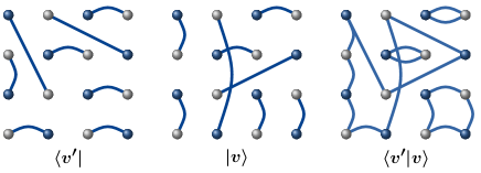
Figure 1: (Color online) Transition graph (right) determining the overlap of two VB states $\left|{v}\right\rangle$ and $\left|{v^{\prime}}\right\rangle$. Note that in the restricted VB basis considered here, all bonds connect sites on different sublattices (with sites on sublattices $\mathcal{A}$ and $\mathcal{B}$ here indicated by darker and lighter circles). The cluster of spins defined by a loop can be in two states, with all spins $\uparrow$ on sublattice $\mathcal{A}$ and $\downarrow$ on $\mathcal{B}$, or vice versa.

II.2 Amplitude-product states

In an amplitude-product state,LIANG1 the expansion coefficients in (3) are products of amplitudes $h({\bf r}_{ij})>0$ (to maintain Marshall’s sign rule for the ground state of a bipartite model),

$$\lambda_{{v}}=\prod_{(i,j)}{h({\bf r}_{ij})},$$ (8)

with the vector ${\bf r}_{ij}$ denoting the “shape” (the lengths in all lattice dimensions) of bond $(i,j)$ in $\left|{{v}}\right\rangle$. This form applies to a translationally invariant system, while in a non-uniform system one should use $h({\bf r}_{i},{\bf r}_{j})$ depending on both end-points of the bonds.

For a given set of amplitudes, the expectation value of some operator $O$ can be written as

$$\langle{O}\rangle=\frac{\langle{\psi_{0}}|{O}|{\psi_{0}}\rangle}{\langle{\psi_{0}}|{\psi_{0}}\rangle}=\frac{\sum_{vv^{\prime}}W_{vv^{\prime}}\frac{\langle{v^{\prime}}|{O}|{v}\rangle}{\langle{v^{\prime}}|{v}\rangle}}{\sum_{vv^{\prime}}W_{vv^{\prime}}},$$ (9)

where the configuration weight is given by

$$W_{vv^{\prime}}=\lambda_{v}\lambda_{v^{\prime}}\,\langle{v^{\prime}}|{v}\rangle=\lambda_{v}\lambda_{v^{\prime}}2^{N_{\circ}-N/2}.$$ (10)

The ratio $\langle{v^{\prime}}|{O}|{v}\rangle/\langle{v^{\prime}}|{v}\rangle$ can normally be related to the loop structure of the transition graph,LIANG1 ; BEACH3 e.g., Eq. (7) in the case of a spin correlation function.

The expectation value (9) is ideally suited for evaluation using Monte Carlo sampling methods,LIANG1 ; LOOP and all the amplitudes can be variationally optimized.LOU ; LOOP Calculations for the Néel-ordered ground state of the 2D Heisenberg model suggest that the fully optimized amplitudes decay as a power-law, $h(|{\bf r}_{ij}|)=1/|{\bf r}_{ij}|^{p}$, with $p\approx 3$.LOOP ; LOU There is reason to believe that the decay exponent in fact is exactly $p=3$, as this is the exponent obtained in an analytical mean-field-like treatment.BEACH1 Some aspects of the critical 1D chain can also be captured with amplitude-product states.BEACH2

The properties of quantum systems are often modified dramatically by introducing quenched (static) randomness: e.g., quantum phase transitions with disorder can lead to new universality classes. For the Heisenberg chain, it is known that any amount of quenched randomness will drive the system into a state well approximated by a random singlet state—a single VB basis state (which is of the “nested” type, with no crossing VBs) with arbitrary VB lengths obtained according to a strong-disorder renormalization-group (SDRG) scheme.DASGUP ; FISHER ; SDRG In this case, the transition-graph loops coincide exactly with the VBs, i.e., $N_{\circ}=N/2$ in (6), and many asymptotic properties follow directly from the length distribution of the VBs.

Amplitude-product states (as well as the special case of the SDRG random singlet states) are useful variational states and we will consider some aspects of their entanglement properties. In many cases completely unbiased results are needed, however. One way to achieve this is with projector QMC simulations in the VB basis, which we briefly discuss next.

II.3 Projector QMC method

In the VB QMC method SANDVIK ; LIANG2 the ground state of the hamiltonian (1) is projected out stochastically, by applying a high power of $H$ to some trial singlet state $\left|{\psi_{t}}\right\rangle$ in the VB basis; $(-H)^{m}\left|{\psi_{t}}\right\rangle\to\left|{\psi_{0}}\right\rangle$ for a large $m$ (up to an irrelevant normalization). A good trial state, such as an optimized amplitude-product state for a uniform system or a single VB state obtained with the SDRG procedure for a 1D random chain, can be used to optimize the convergence properties of such a scheme, but the final result is not sensitive to $\left|{\psi_{t}}\right\rangle$ as long as $m$ is sufficiently large (i.e., the method is unbiased).

There are two formulations of the VB QMC method,SANDVIK generating either the ground state wave function or the ket and bra versions of the ground state needed to evaluate expectation values. In the former case, stochastic application of the projector $H^{m}$ (for sufficiently large $m$) on the trial state produces VB basis states distributed proportionally to the expansion coefficients $\lambda_{v}$ in (3), i.e., these coefficients are not known (and would be much more complicated than the simple amplitude products) but importance-sampling of the contributions to $H^{m}|\psi_{t}\rangle$, which resemble terms in a path integral, generate them probabilistically (with many paths contributing to a single coefficient $\lambda_{v}$).

In the “double projection” method, an expectation value is formally given by Eq. (9), but the expansion coefficients $\lambda_{v}$ are again not known. The sampling of paths obtained from the combined ket $H^{m}\left|{\psi_{t}}\right\rangle$ and bra $\left\langle{\psi_{t}}\right|H^{m}$ states, i.e., $\left\langle{\psi_{t}}\right|H^{2m}\left|{\psi_{t}}\right\rangle$, leads to a series of VB-pair configurations distributed according to the weights $W_{vv^{\prime}}$ in (10).

In both the wave-function and expectation-value projection schemes, one can employ efficient loop updates for generating the states and transition graphs, as discussed in detail in Ref. LOOP, . In the sampling procedures of such algorithms, one uses the combined spin-bond basis and applies a high power ${H}^{m}$ or ${H}^{2m}$ in a way similar to the ”operator-loop” update in the finite temperature stochastic series expansion QMC method.SSE The computational effort scales as $\mathcal{O}(m)$, and to converge calculated quantities to the ground state $m$ has to be scaled as $\propto N^{a}$, with $a$ typically in the range $1-2$ (depending on the model’s low-energy energy spectrum and the quality of the trial state $|\psi_{t}\rangle$).LOOP

II.4 Loop-gas description

The loop-gas view of VB sampling was suggested by Sutherland some time ago.SUTHER1 ; SUTHER2 Consider the two VB configurations in a transition graph $\langle v^{\prime}|v\rangle$ with the associated weight (10) for an amplitude-product state. In that case, the factor $\lambda_{v}\lambda_{v^{\prime}}$ does not depend on details of the bond arrangements, only on the total number $N_{b}({\bf r})$ of bonds of all shapes ${\bf r}$ in the two states $|v\rangle$ and $|v^{\prime}\rangle$ (i.e., no bond correlations are included). In addition to the factor $2$ in the overlap (6) for each loop in the transition graph, for each loop containing more than two bonds we can consider swapping all bonds belonging to a given loop between $|v\rangle$ and $|v^{\prime}\rangle$, as illustrated in Fig. 2. This swapping does not affect the weight (10) of the joint configuration of the two states (although the weights $\lambda_{v}$ and $\lambda_{v^{\prime}}$ of the individual states are affected). The two bond configurations and two staggered spin patterns for each loop corresponds to a loop fugacity $4$ for all loops of length $4$ or larger. The shortest, length-$2$, loops have fugacity $2$, as the bond swapping in this case does not affect the bond configurations.

Instead of sampling bonds weighted according to (10), one can think of sampling loops with the weight

$$W=2^{N_{\circ}(2)}4^{N_{\circ}(>2)}\prod_{\bf r}h({\bf r})^{N_{b}({\bf r})},$$ (11)

where $N_{\circ}(2)$ and $N_{\circ}(>2)$ denote the number of loops of length $2$ and larger than $2$, respectively, and the unimportant factor $2^{-N/2}$ in (6) has been omitted. The product of amplitudes can here be thought of as originating from the shapes of the loops. In special cases, such as Anderson’s resonating valence-bond (RVB) state including only the shortest bonds (of length $r=1$),RVB ; ALBU ; TANG the weight only depends on the number of loops. This was the case considered by Sutherland,SUTHER2 who also studied generalizations of the loop gas in which the loop fugacities, $Z_{2}=2$ and $Z_{>2}=4$ in (11), can take arbitrary values and, thus, phase transitions can be studied as a function of these fugacities.

The loop-gas weight function (11) does not apply to states beyond the amplitude-product description. In the exact ground state of a given hamiltonian, one would in general expect bond correlations. The product of two VB expansion coefficients in (10) then changes when an intra-loop bond swap of the type illustrated in Fig. 2 is carried out, thus invalidating the form (11). One can still, however, sum up the weights obtained as a result of all such bond swaps which leave the loop structure intact, and this way, in principle (but hardly in practice), write down a weight for a loop configurations which is more complicated than (11). The loop configurations generated in the QMC projector method represent a stochastic implementation of this more general loop-gas picture. Note that even in this generalization, each loop is associated with a factor of two arising from the two allowed staggered spin configurations of the cluster of sites defined by the loop.

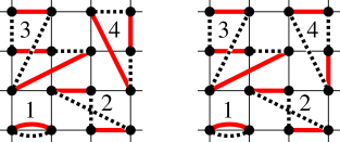
Figure 2: (Color online) Two transition graphs $\langle v^{\prime}|v\rangle$ with the same loops structure (with four loops, labeled 1,2,3,4). The two cases shown here illustrate how bonds within a loop (here loop 4) can be swapped between $|v\rangle$ and $\langle v^{\prime}|$ (represented by solid and dashed bonds, respectively). This kind of bond reconfiguration leaves the weight unchanged in the case of an amplitude-product state, but not in a more general state in which there are correlations between the bonds.

III Valence-bond entanglement entropy

A singlet state formed by two $S=1/2$ spins is maximally entangled and has the maximum value of the von Neumann bipartite entanglement entropy; $S_{\text{vN}}=1$ (measured in bits). The simplest case for computing $S_{\text{vN}}$ of a many-body system is a single VB basis state $\left|{v}\right\rangle$. For a given bipartition, its entanglement entropy is just the number of singlets $n_{AB}$ connecting subsystems $\mathcal{A}$ and $\mathcal{B}$.REFAEL It is not easy to compute $S_{\text{vN}}$ for a superposition of VB states, however. In Refs. VBE1, and VBE2, a straight-forward generalization of the result for a single VB state was proposed as an alternative definition of entanglement entropy for an arbitrary superposition of VB states, using the average number of bonds connecting the two subsystems. With the VB projector method for the wave function, one stochastically evaluates

$$S_{\text{VB}}^{1}=\frac{\sum_{v}\lambda_{v}n_{AB}}{\sum_{v}\lambda_{v}}.$$ (12)

Here we investigate a different definition, using the expectation value

$$S_{\text{VB}}^{2}=\langle n_{\rm AB}\rangle,$$ (13)

evaluated using Eq. (9) with $O=n_{\rm AB}$. Here it should be noted that we define $n_{\rm AB}$ as just counting of the bonds crossing the two subsystems, and that this counting can be performed in the transition graph of $\langle v^{\prime}|v\rangle$ either in $|v\rangle$ or $\langle v^{\prime}|$. For a given configuration these numbers are different (i.e., the operator is not hermitian), but the averages are the same. In Sec. V we will address further potential problems in interpreting $\langle n_{\rm AB}\rangle$ as a standard quantum mechanical expectation value. For now, we consider this quantity as an interesting aspect of the transition graphs, the statistical properties of which are uniquely determined for a given hamiltonian with short-range interactions (as we will further argue in Sec. V).

For a single VB state $S_{\text{VB}}^{2}=S_{\text{VB}}^{1}$, but in a superposition these quantities are different, because of the over-completeness and associated different weighting of the VB configurations. We next present projector QMC results for both $S_{\text{VB}}^{1}$ and $S_{\text{VB}}^{2}$ in 1D and 2D Heisenberg systems and discuss their scaling as a function of the size of the smaller subsystem of the bipartition.

III.1 Homogeneous chain

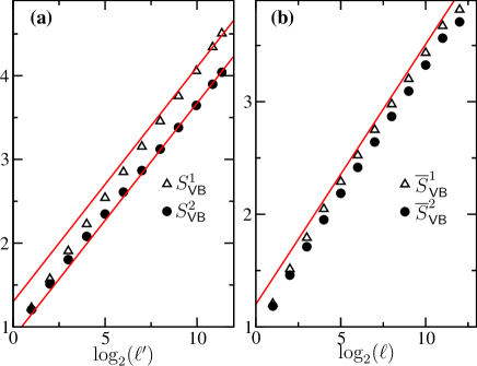
Figure 3: (Color online) (a) VB entropies for subsystems of size $\ell$ in a Heisenberg chain of length $L=2^{13}$ as a function of the logarithm of the conformal distance; $\log_{2}(\ell^{\prime})=\log_{2}[(L/\pi)\sin(\pi\ell/L)]$. The lines have slope $\gamma=4\ln(2)/\pi^{2}$, as in the exact asymptotic form.JACOBSEN (b) Disorder-averaged VB entropies for the 1D random chain, as a function of $\log_{2}(\ell)$. The line has slope $\gamma=\ln(2)/3$.

We consider first the standard Heisenberg chain with uniform interactions. For a large segment of size $\ell$, embedded in a chain of length $L$, the von Neumann entanglement entropy has the asymptotic behavior $S_{\text{vN}}(\ell)=(c/3)\log_{2}(\ell^{\prime})+s_{0}$, where $\ell^{\prime}=(L/\pi)\sin(\pi\ell/L)$ is the conformal length, $c=1$ is the central charge, and $s_{0}$ is a non-universal constant.CARDY The VB entropy $S^{1}_{\rm VB}$ is known to diverge in the same way, but with a different factor, $\gamma=4\ln(2)/\pi^{2}\approx 0.281$.JACOBSEN Previous calculations are consistent with $\gamma<1/3$ for large chains,LADDER but, as can be seen in Fig. 3(a) for a chain of $2^{13}$ spins, there are still large non-asymptotic corrections which make it difficult to verify the factor precisely.CAPPONI On the other hand, our results for $S_{\text{VB}}^{2}$ are completely consistent with the known $\gamma$ over a large range of subsystems. This may appear surprising, because the exact calculation is based on the wave-function definition $S^{1}_{\rm VB}$,JACOBSEN not the expectation value $S^{2}_{\rm VB}$. It is plausible, however, that $S^{1}_{\rm VB}$ and $S^{2}_{\rm VB}$ scale asymptotically with the same $\gamma$ (with different additive constants), but that $S^{2}_{\rm VB}$ is less affected by subleading scaling corrections.

III.2 Disordered chain

Now we turn to the disordered chain, with random couplings generated from the uniform distribution in the interval $(0,1]$. The ground state of this system is known to be well approximated by a random singlet, where all spins form a single non-crossing VB state with arbitrary bipartite bond lengths.FISHER Using an SDRG analysis, Refael and Moore REFAEL showed that the disorder average of the von Neumann entanglement entropy $\overline{S}_{\text{vN}}$ in such a state scales logarithmically with a universal coefficient $\gamma=\ln(2)/3$. This result should hold also for the VB entanglement entropy of the Heisenberg chain when $L\to\infty$, although the ground state is not exactly a single VB basis state—there are fluctuations around the dominant SDRG configuration.TRAN Our results for both $S^{1}_{\rm VB}$ and $S^{2}_{\rm VB}$, shown in Fig. 3(b), are consistent with $\gamma=\ln(2)/3$ (considering some remaining finite-size effects for the largest subsystems).

III.3 Two-dimensional system

We next consider the 2D Heisenberg model, which we have studied on $L\times L$ lattices with $L$ up to $256$. Fig. 4 shows results for $S_{\text{VB}}^{2}(\ell)$ of square subsystems of linear size $\ell$. The data converge very rapidly with $L$ for $\ell\leq L/4$. There is clearly a multiplicative logarithmic correction to the area law, $S_{\text{VB}}^{2}(\ell)/\ell\propto\log_{2}(\ell)$, as found previously for $S_{\text{VB}}^{1}$ in Refs. VBE1, ; LADDER, . Both VB entropy definitions, thus, violate the area law in this case. The von Neumann entropy, on the other hand, should obey the area law, $S_{\text{vN}}(\ell)\propto\ell$, although, because of difficulties in calculating this quantity in an unbiased way, it has not been possible to confirm it unambiguously.LADDER The recent calculation of the Rényi entropy $S_{2}$ is, however, in agreement with the area law.RENYI

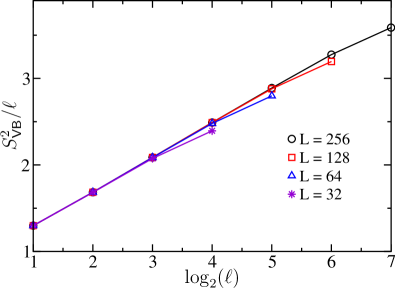
Figure 4: (Color online) The VB entropy $S_{\text{VB}}^{2}$ divided by the linear dimension $\ell$ of a square sub-block in 2D $L\times L$ lattices with $L=32-256$.

We conclude that $S_{\text{VB}}^{2}$ has an advantage over $S_{\text{VB}}^{1}$, in the sense that its logarithmic prefactor in 1D converges faster to the result of the exact calculation in Ref. JACOBSEN, (although we do not know whether the faster convergence is generic). Neither of these definitions serves well as a proxy for the von Neumann entanglement entropy $S_{\text{vN}}$, however, because the area law is violated in 2D by a multiplicative logarithmic correction. Only additive corrections to the area law are expected.CASINI ; RYU

IV Loop entanglement entropy

The loop-gas picture discussed in Sec. II.4 suggests a potential reason why the VB entanglement entropies (12) and (13) violate the area law in 2D systems: The VB basis consists of singlet pairs, but when considering an expectation value, constraints related to the over-completeness are imposed on the spin states beyond the singlet pairing. These constraints are similar to multi-spin entanglement, as there are two spin states for each loop (the two staggered spin configurations on the loops) and these loops are, thus, analogous to maximally entangled sets of spins (albeit in an overlap matrix element, not a wave function). All bonds therefore do not carry a full unit of entanglement entropy (because they are entangled with other bonds in the same loop), and the VB entropy $S_{\text{VB}}^{2}$ may therefore overestimate the actual entanglement entropy. This could also be the case with $S_{\text{VB}}^{1}$, because it, too, is based on a superposition of states with only pair-wise entanglement (and, as we showed in Sec. III, $S_{\text{VB}}^{1}$ and $S_{\text{VB}}^{2}$ have the same scaling properties). On the other hand, in 1D $S_{\text{VB}}^{1}$ and $S_{\text{VB}}^{2}$ actually underestimate the entanglement entropy (in relation to the von Neumann entanglement entropy, which is slightly larger than the bond entropies in this case). The intuitive picture of entanglement entropy in terms of bonds is therefore, as a consequence of the overcompleteness, not always quantitatively correct.

We will here consider a measure of entanglement entropy $S_{\rm loop}$ in terms of shared loops in the transition graph, as illustrated in Fig. 5. Since the number of shared loops must be smaller or equal to the number of shared bonds, we have $S_{\rm loop}\leq S_{\text{VB}}^{2}$, and it is therefore clear that $S_{\rm loop}$ cannot be a better approximation to $S_{\rm vN}$ than $S_{\text{VB}}^{2}$ in the case of the 1D Heisenberg chain. We will be mainly interested in $S_{\rm loop}$ of the 2D system, but will also investigate it in 1D.

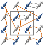
Figure 5: (Color online) The loop entropy $S_{\text{loop}}$ of a subsystem (gray square) is defined as the average number of loops in the transition graph shared by the subsystem and the rest of the system. In this example two loops are shared.

Before discussing the actual definition of $S_{\rm loop}$ further, let us consider for a moment the wave function. Instead of a bond-singlet pairing of the spins, one might regard a state as a superposition of products of loop-cluster states,

$$|\Psi\rangle=\sum_{\alpha}\bigotimes_{i=1}^{N_{\alpha}}|\psi(i)\rangle_{\alpha},$$ (14)

where $N_{\alpha}$ is the number of loops in component $\alpha$ and an individual cluster state of $n$ spins is of the form

$$|\psi(i)\rangle_{\alpha}=\frac{1}{\sqrt{2}}\left(\left|{\uparrow_{1}\downarrow_{2}\cdots\downarrow_{n}}\right\rangle_{\alpha}^{i}-\left|{\downarrow_{1}\uparrow_{2}\cdots\uparrow_{n}}\right\rangle_{\alpha}^{i}\right).$$ (15)

This is a maximally entangled state of two staggered spin configurations along the loop of $n$ spins (or, equivalently, all even numbered spins are on sublattice $\mathcal{A}$ and all odd ones on $\mathcal{B}$, or vice versa). With such as loop-cluster wave function, it is natural to regard a loop shared by two subsystems in a bipartition as carrying one unit of entanglement entropy. Thus, we define the loop entanglement entropy as

$$S_{\rm loop}=\langle\Lambda_{AB}\rangle,$$ (16)

where $\Lambda_{AB}$ counts the number of loops shared by subsystems $A$ and $B$ (i.e., loops passing through both the subsystems) in a given bipartition.

The loop-cluster view of entanglement entropy is realized in SDRG calculations for the random transverse-field Ising model,LIN where the clusters have parallel spins and the ground state is given by a single product of such cluster states. The generalization to a superposition of cluster products has the same motivation as the generalization of the entanglement entropy of the single VB state appearing in the SDRG scheme for the random Heisenberg chain REFAEL to a superposition.VBE1 ; VBE2 In general, it is not known, however, how to write the wave function of a Heisenberg system as a superposition of cluster states (and clearly there is no unique way of doing so, as such a basis is massively overcomplete). As we have seen, such loop-cluster superpositions do appear in the loop-gas picture, and it is then natural to define $S_{\rm loop}$ as above using the transition graph loops, as illustrated in Fig. 5. We will explore this measure of entanglement here.

One may again question whether an expectation value such as $\langle\Lambda_{AB}\rangle$ is a bona fide quantum mechanical expectation value. We will discuss this further in Sec. V and here only consider it, like $S^{2}_{\rm VB}$, as a statistical property of the transposition graphs generated in the projector QMC scheme (or in sampling of an amplitude-product state, which we will also investigate).

Clearly, the loop entropy is a boundary property, and we can write either $S_{\rm loop}(A)$ or $S_{\rm loop}(B)$ for a bipartition $(A,B)$. It is easy to demonstrate the sub-additive property $S_{\rm loop}(A_{1}\cup A_{2})\leq S_{\rm loop}(A_{1})+S_{\rm loop}(A_{2})$ for two different bipartitions, $(A_{1},B_{1})$ and $(A_{2},B_{2})$. The essential properties of an entropy are thus satisfied. For a single VB configuration, loops and bonds coincide and, thus, $S_{\rm loop}=S^{1}_{\rm VB}=S^{2}_{\rm VB}=S_{\rm vN}$ in this case.

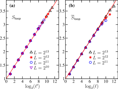
Figure 6: (Color online) Loop entropy of Heisenberg chains with (a) uniform and (b) random couplings (versus the logarithms of the conformal and linear subsystem sizes, respectively). Both lines have slope $\gamma=\ln(2)/3$.

IV.1 1D and 2D Heisenberg models

We first consider the loop entropy for ground states of Heisenberg models obtained by the projector QMC method. Figs. 6 and 7 show results for 1D and 2D systems, respectively. Interestingly, in 1D, the behavior is consistent with a logarithmic divergence with a prefactor $\gamma=\ln(2)/3\approx 0.231$ (to within a statistical error of about 1%) for both the uniform and random chains (with uniformly distributed couplings between $0$ and $1$), i.e., the same as the bond-based entropy for the random chain (Fig. 3). The result is expected for the random chain, because the asymptotic SDRG state of such a system is a single VB state, in which $S_{\rm loop}=S^{1}_{\rm VB}=S^{2}_{\rm loop}$ (and this is the exact result), but it is curious that the same value obtains for the uniform chain as well. This may also be taken as a flaw of the loop-based entropy (if one wants a a quantity mimicking the von Neumann entropy as closely as possible), because it is further from $S_{\rm vN}$ ($\gamma=1/3$) than the bond-based estimates ($\gamma=4\ln(2)/\pi^{2}\approx 0.281$). Nevertheless, it is encouraging that the logarithmic divergence is still captured.

In the 2D system, $S_{\rm loop}/\ell$ converges to a finite value with increasing $\ell$ and $L$. Note the rapid convergence as a function of the full system size in Fig. 7. For the largest system ($L=256$) the results are described very well by an area law with an additive logarithmic correction; $S_{\text{loop}}=\mu\ell+a\log_{2}(\ell)+s_{0}$. The area law prefactor $\mu\approx 0.51$ is, intriguingly, in good agreement with $S_{\rm vN}/\ell$ obtained by Kallin et al. LADDER for wide ladder systems [accounting for the $\ln(2)$ included there in the definition of $S_{\rm vN}$]. In this case the loop entropy is, thus, a better stand-in for $S_{\rm vN}$ (which is expected to obey the area law) than the bond-based quantities.

Note that the presence of long-range Néel order in 2D implies the existence of system-spanning loops in the transition graph.LOOP This explains why $S_{\rm loop}$ is much smaller than $S^{2}_{\rm VB}$ in Fig. 5 (i.e., because of the large average loop size, the number of loops in the transition graph is much smaller than the number of bonds).

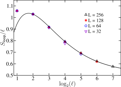
Figure 7: (Color online) The loop entropy divided by the linear dimension $\ell$ of a square sub-block in several $L\times L$ lattices. The curve shows a fit of the $L=256$ data ($\ell\geq 2^{2}$) to the form $S_{\text{loop}}=\mu\ell+a\log_{2}(\ell)+s_{0}$, with $\mu\approx 0.51$, $a\approx 1.12$, and $s_{0}\approx-0.34$. The quality of this fit is statistically sound, with $\chi^{2}/{\rm dof}<1$ when $\ell\geq 8$ data are included. The error bars are much smaller than the symbols, of the order $10^{-4}$ for $S_{\rm loop}/\ell$.

IV.2 Néel-ordered 2D amplitude-product state

We also investigate the scaling behavior of the loop entropy for a 2D amplitude product state, (4) with the expansion coefficients given by (8) with $h(r)=1/r^{3}$. This corresponds to the asymptotic form of the optimal variational amplitudes for the 2D Heisenberg model suggested by previous calculations.LOOP ; LOU We here do not use fully optimized amplitudes (which show deviations from the $1/r^{3}$ for short bonds), because our aim is to investigate a generic Néel-ordered state, to compare with the results of the specific case of the ground state if the 2D Heisenberg model in Fig. 7.

The sublattice magnetization in the amplitude-product state with $h(r)=1/r^{3}$ for all $r$ is $m_{s}\approx 0.27$ (extracted from the system size dependence of $\langle m_{s}^{2}\rangle$ for systems of size $L$ up to $256$), somewhat below the known value $m_{s}\approx 0.307$ for the Heisenberg model. The results in Fig. 8 show a behavior very similar to the Heisenberg ground state result in Fig. 7, with a correction to the area law which can be described as an additive logarithm. Because of the lower value of the sublattice magnetization, the average loop size is smaller, and, thus, the number of loops in the system (including those shared by the two subsystems) is larger, leading to higher overall value of $S_{\rm loop}$ than in Fig. 5.

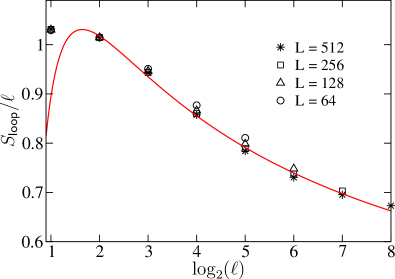
Figure 8: (Color online). Loop entropy of the amplitude-product state with amplitudes decaying with the bond length $r$ as $h(r)=1/r^{3}$, which is the asymptotic form in the optimal amplitude product state for the 2D Heisenberg model.LOU The entropy divided by the system length saturates for large systems, indicating applicability of the area law (with an additive logarithmic correction described by the same form as in Fig. 7; a fit is indicated by the solid curve).

V Summary and discussion

Using the transition graphs characterizing state overlaps in the valence bond basis of $S=1/2$ spins, we have explored two measures of bipartite entanglement entropy, $S_{\text{VB}}^{2}$ and $S_{\text{loop}}$. The former extends the definition $S_{\text{VB}}^{1}$ of valence-bond entropy (Refs. VBE1, ; VBE2, ) based on shared valance bonds in the wave function to the transition graph, while the latter is based on shared loops (motivated by the loop-gas picture SUTHER1 ; SUTHER2 of spin systems). Using an efficient loop algorithm,LOOP we were able to obtain unbiased QMC results for these quantities in large systems; $2^{13}$ and $2^{16}$ spins in 1D and 2D, respectively.

In the Heisenberg chain, $S^{2}_{\text{VB}}$ exhibits a logarithmic divergence, with a prefactor which agrees well with the exact valueJACOBSEN $\gamma=4\ln(2)/\pi^{2}$ already for small subsystems. In contrast, observing this scaling with the wave-function definition $S^{1}_{\text{VB}}$ VBE1 ; LADDER requires very large systems, due to significant subleading corrections.CAPPONI

For the Néel state of the 2D Heisenberg model, both VB entropies violate the area law, exhibiting multiplicative logarithmic corrections.VBE1 We have argued that single-bond definitions typically overestimate the amount of entanglement, because of the over-completeness of the VB basis. The loop definition $S_{\rm loop}$ exhibits only an additive size correction to the area law in 2D, in agreement with general expectations for standard definitions.CASINI ; RYU ; RENYI

Important relationships have been established in recent years between the subleading behavior of the entanglement entropy, topological order, and quantum-criticality. For instance, the subleading term in a 2D gapped system is a constant determined by the quantum dimension of the excitations of the topological phase.KITAEV ; LEVIN For critical systems in the universality class of $z=2$ conformal quantum-critical points, there is a universal additive logarithmic subleading term, which depends only on the shape of the subsystem partition and the central charge.FRADKIN An additive correction to the area law in the 2D Néel state was also found for the Rényi entropy $S_{2}$, but the systems were too small to determine its asymptotic form.RENYI We have shown that the loop entropy $S_{\rm loops}$ captures the essential desired features of an entanglement entropy, scaling logarithmically with the subsystem size in 1D and obeying the area law for the 2D Néel state. Being relatively easy to calculate, S_loops offers opportunities to study various aspects of entanglement entropy on large spin lattices in other situations of great interest, e.g., at unconventional quantum-critical points.SENTHIL ; JQLOGS

In Sec. III we already commented on the fact that properties such as $S_{\rm VB}^{2}$ and $S_{\rm loop}$ that are defined using specific geometrical properties of the transition graphs (i.e., not following directly from a given operator acting on the spins) in the valence bond basis are not necessarily well defined expectation values of some hermitian operators. Indeed, it has recently been shown that the entanglement entropies defined in this way are dependent on exactly how a state is represented in the overcomplete valence bond basis.MAMBR This may suggest that these quantities are ill-defined. However, given a hamiltonian $H$, the projector QMC method generates the transition graphs in a unique way, independently of the trial state used (which we have also verified explicitly).

The valence-bond projector technique itself is closely tied to the completely generic “loop-operator” representation of the path integral for a singlet state,NACHT ; LOOP and therefore the statistical properties of the transition graph loops (including $S_{\rm VB}^{2}$ and $S_{\rm loop}$) are not really tied to the particular QMC scheme, only to the valence-bond basis. The definitions are tied to the hamiltonian, in the sense that $H$ generates the transition graphs. We can therefore not, in general, evaluate $S_{\rm VB}^{2}$ and $S_{\rm loop}$ uniquely just based on an arbitrary state, but first need to find the “parent hamiltonian” of the state (and furthermore, that parent hamiltonian should have short-range interactions only, so that it is unique—support for this generic statement is discussed in Ref. VERST, ), and use it to generate the transition graphs. States defined based on “unbiased” bond superpositions (which includes contributions from all different ways of expressing the state in terms of singlets obeying Marshall’s sign rule), such as the amplitude-product states (and perhaps generalizations of them including bond correlations) can also be studied, as we have done here in a 2D case (and where it is important to note that for such a state with Néel order, we obtained results in good agreement with the projected ground state of the 2D Heisenberg model). In practice, we expect $S_{\rm VB}^{2}$ and $S_{\rm loop}$ to be useful primarily in QMC studies of ground states of specific hamiltonians.

In the loop-operator formulation,NACHT ; LOOP one can think of clusters of spins (defined by transition-graph loops) as forming dynamically in imaginary time. The entanglement entropies $S_{\rm VB}^{2}$ and $S_{\rm loop}$ correspond to entropy measurements averaged over equal-time “snapshots” of entangled clusters in this time evolution. Exactly how this dynamic aspect relates to the standard wave-function picture of entanglement entropy is not clear at present, but the results obtained in this paper suggest that there should be a close relationship between them.

References

- (1) J. Eisert, M. Cramer, M. B. Plenio, Rev. Mod. Phys. 82, 277 (2010).
- (2) M. Srednicki, Phys. Rev. Lett. 71, 666 (1993).
- (3) A. Kitaev and J. Preskill, Phys. Rev. Lett. 96, 110404 (2006).
- (4) M. M. Wolf, F. Verstraete, M. B. Hastings, and J. I. Cirac, Phys. Rev. Lett. 100, 070502 (2008).
- (5) M. Levin and X.-G. Wen, Phys. Rev. Lett. 96, 110405 (2006).
- (6) E. Fradkin and J. E. Moore, Phys. Rev. Lett. 97, 050404 (2006).
- (7) J. I. Cirac and F. Verstraete, J. Phys. A: Math. Theor. 42, 504004 (2009).
- (8) L. Tagliacozzo, G. Evenbly, and G. Vidal, Phys. Rev. B 80, 235127 (2009).
- (9) U. Schollwöck, Rev. Mod. Phys. 77, 259 (2005).
- (10) A. B. Kallin, I. Gonzalez, M. B. Hastings, R. G. Melko, Phys. Rev. Lett. 103, 117203 (2009).
- (11) H. Li and F. D. M. Haldane, Phys. Rev. Lett. 101, 010504 (2008).
- (12) M. B. Hastings, I. González, A. B. Kallin, and R. G. Melko, Phys. Rev. Lett. 104, 157201 (2010).
- (13) A. W. Sandvik, Phys. Rev. Lett. 95, 207203 (2005).
- (14) F. Alet, S. Capponi, N. Laflorencie, and M. Mambrini, Phys. Rev. Lett. 99, 117204 (2007).
- (15) R. W. Chhajlany, P. Tomczak, and A. Wójcik, Phys. Rev. Lett. 99, 167204 (2007).
- (16) G. Refael and J. E. Moore, Phys. Rev. Lett. 93, 260602 (2004).
- (17) F. Alet, I. P. McCulloch, S. Capponi, and M. Mambrini, Phys. Rev. B 82, 094452 (2010).
- (18) J. L. Jacobsen and H. Saleur, Phys. Rev. Lett. 100, 087205 (2008).
- (19) A. W. Sandvik and H. G. Evertz, Phys. Rev. B 82, 024407 (2010).
- (20) S. Liang, B. Doucot, and P. W. Anderson, Phys. Rev. Lett. 61, 365 (1988).
- (21) B. Sutherland, Phys. Rev. B 37, 3786 (1988).
- (22) B. Sutherland, Phys. Rev. B 38, 6855 (1988).
- (23) W. Marshall, Proc. Roy. Soc. A 232, 48 (1955).
- (24) K. S. D. Beach and A. W. Sandvik, Nucl. Phys. B 750, 142 (2005).
- (25) J. Lou and A. W. Sandvik, Phys. Rev. B 76, 104432 (2007).
- (26) K. S. D. Beach, Phys. Rev. B 79, 224431 (2009).
- (27) K. S. D. Beach, arXiv:0709.4487.
- (28) C. Dasgupta and S.-K. Ma, Phys. Rev. B 22, 1305 (1980).
- (29) D. S. Fisher, Phys. Rev. B 50, 3799 (1994).
- (30) F. Iglói and C. Monthus, Phys. Rep. 412, 277 (2005).
- (31) S. Liang, Phys. Rev. B 42, 6555 (1990).
- (32) A. W. Sandvik, Phys. Rev. B 59, 14157(R) (1999).
- (33) P. Fazekas and P. W. Anderson, Philos. Mag. 30, 423 (1974); P. W. Anderson, Science 235 1196 (1987).
- (34) A. F. Albuquerque and F. Alet, Phys. Rev. B 82, 180408 (2010).
- (35) Y. Tang, A. W. Sandvik, and C. L. Henley, arXiv:1010.6146.
- (36) P. Calabrese and J. Cardy, J. Stat. Mech. Theor. Exp. (2004), P06002.
- (37) H. Tran and N. E. Bonesteeel, arXiv:0909.0038.
- (38) H. Casini and M. Huerta, Nucl. Phys. B 764, 183 (2007).
- (39) S. Ryu and T. Takayanagi, Phys. Rev. Lett. 96, 181602 (2006).
- (40) Y.-C. Lin, F. Iglói, and H. Rieger, Phys. Rev. Lett. 99, 147202 (2007).
- (41) T. Senthil, A. Vishwanath, L. Balents, S. Sachdev, and M. P. A. Fisher, Science 303, 1490 (2004).
- (42) A. W. Sandvik, Phys. Rev. Lett. 104, 177201 (2010).
- (43) S. Capponi, F. Alet, M. Mambrini, arXiv:1011.6530 (unpublished).
- (44) M. Aizenman and B. Nachtergaele, Comm. Math. Phys. 164, 17 (1994).
- (45) F. Verstraete and J. I. Cirac, Phys. Rev. B 73, 094423 (2006).